Individual Tree Diameter Growth Models of Larch–Spruce–Fir Mixed Forests Based on Machine Learning Algorithms


Abstract
1. Introduction
2. Data and Methods
2.1. Data
2.1.1. Study Area
2.1.2. Permanent Plot Data
2.1.3. Climate Data
2.2. Modelling Techniques
2.2.1. Modelling Methods and Development
2.2.2. Model Evaluation
2.3. Model Comparison
3. Results
3.1. Individual Tree Diameter Prediction Based on ML Algorithms
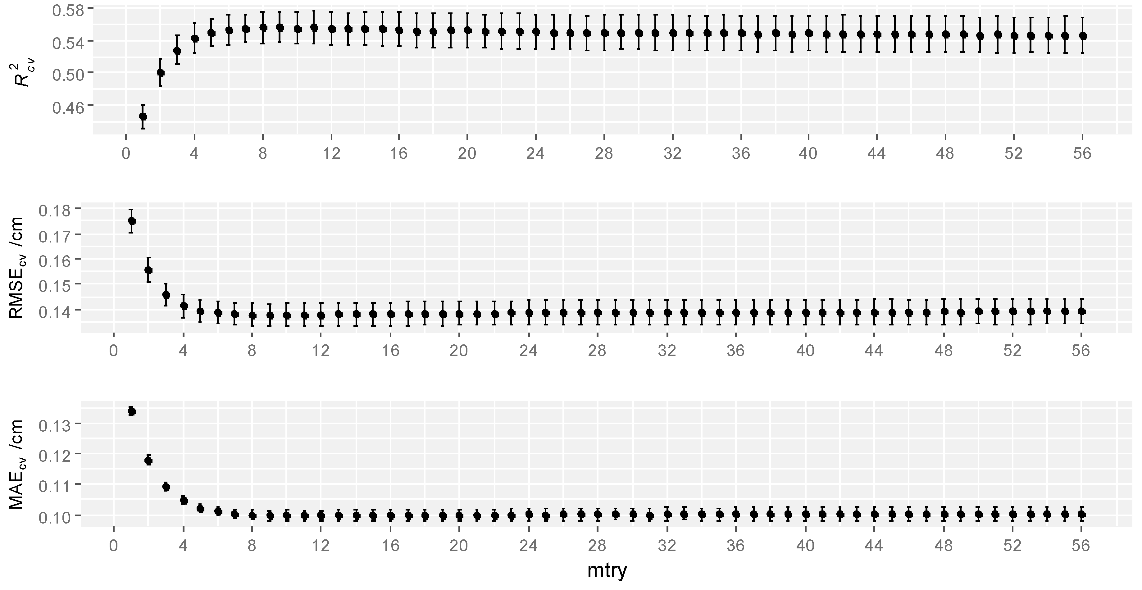
3.1.1. RF
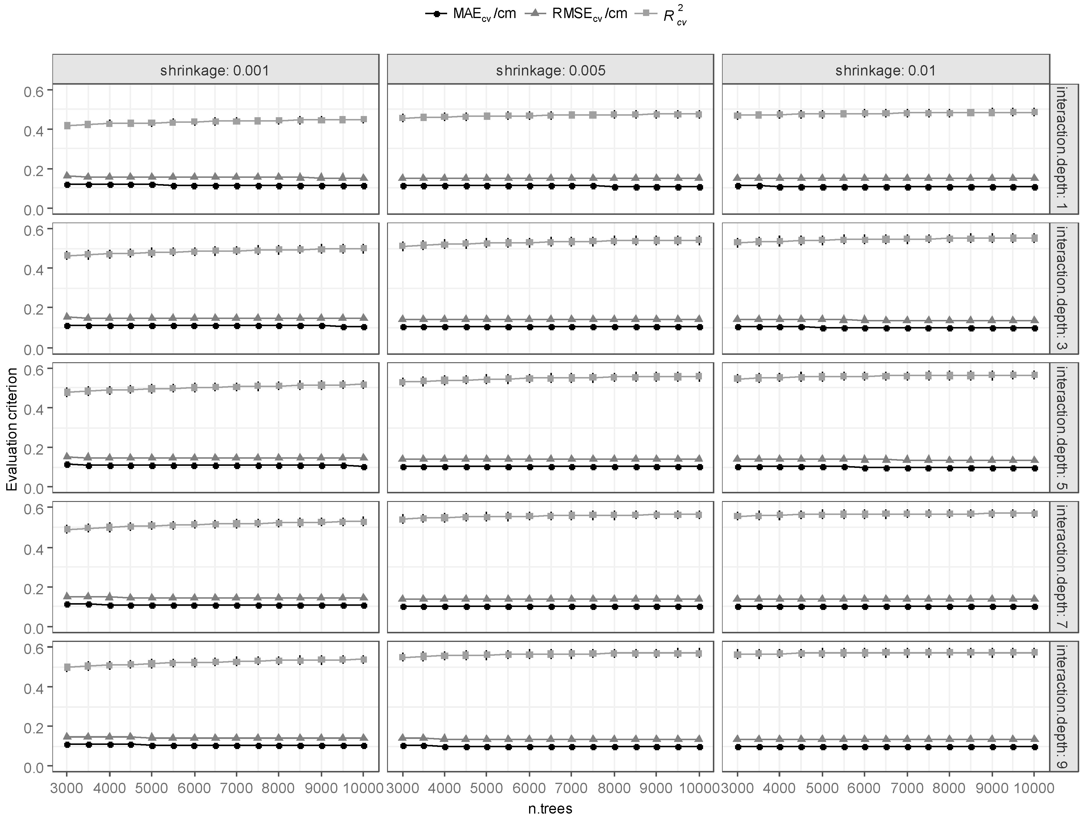
3.1.2. BRT
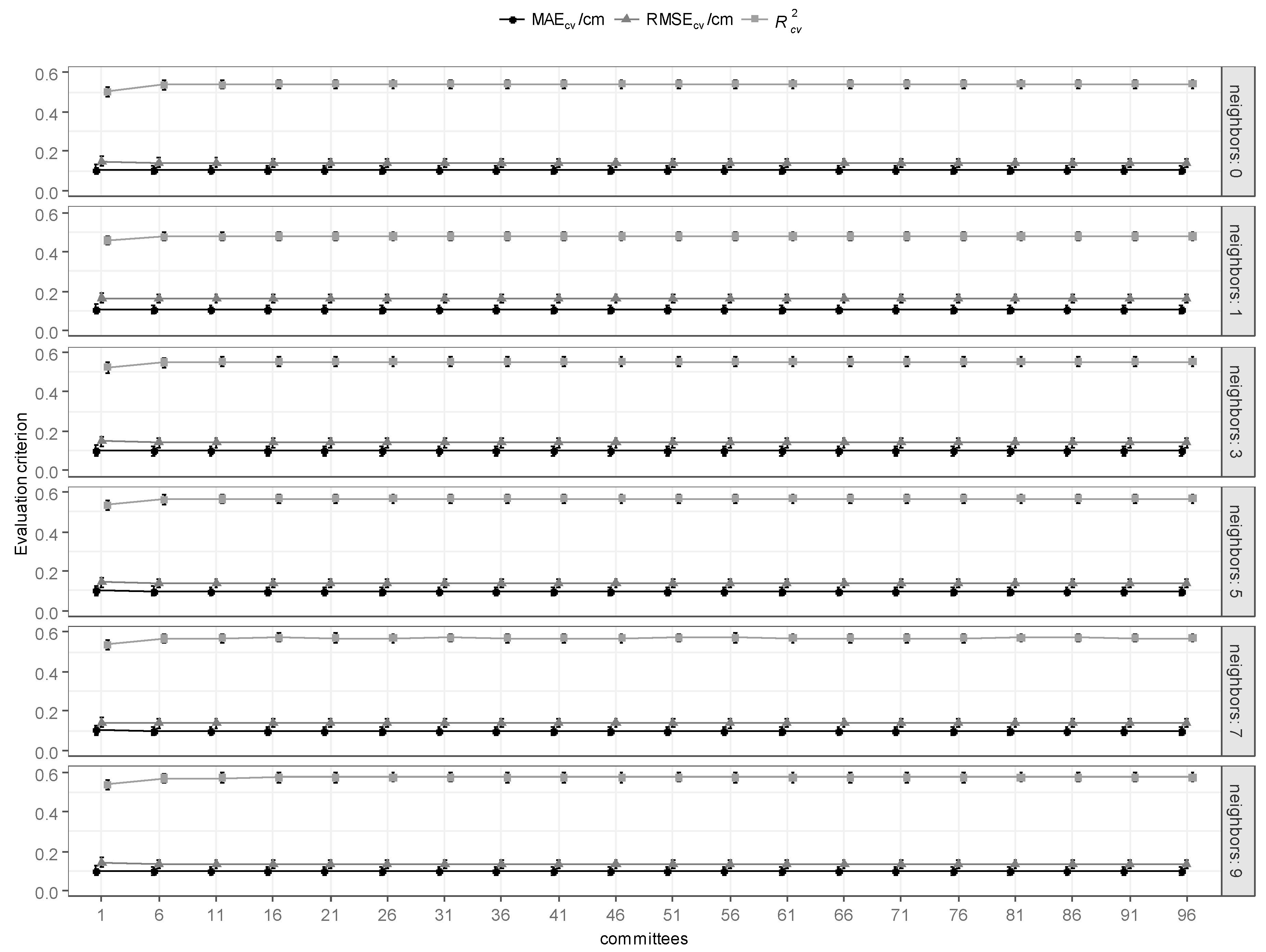
3.1.3. Cubist
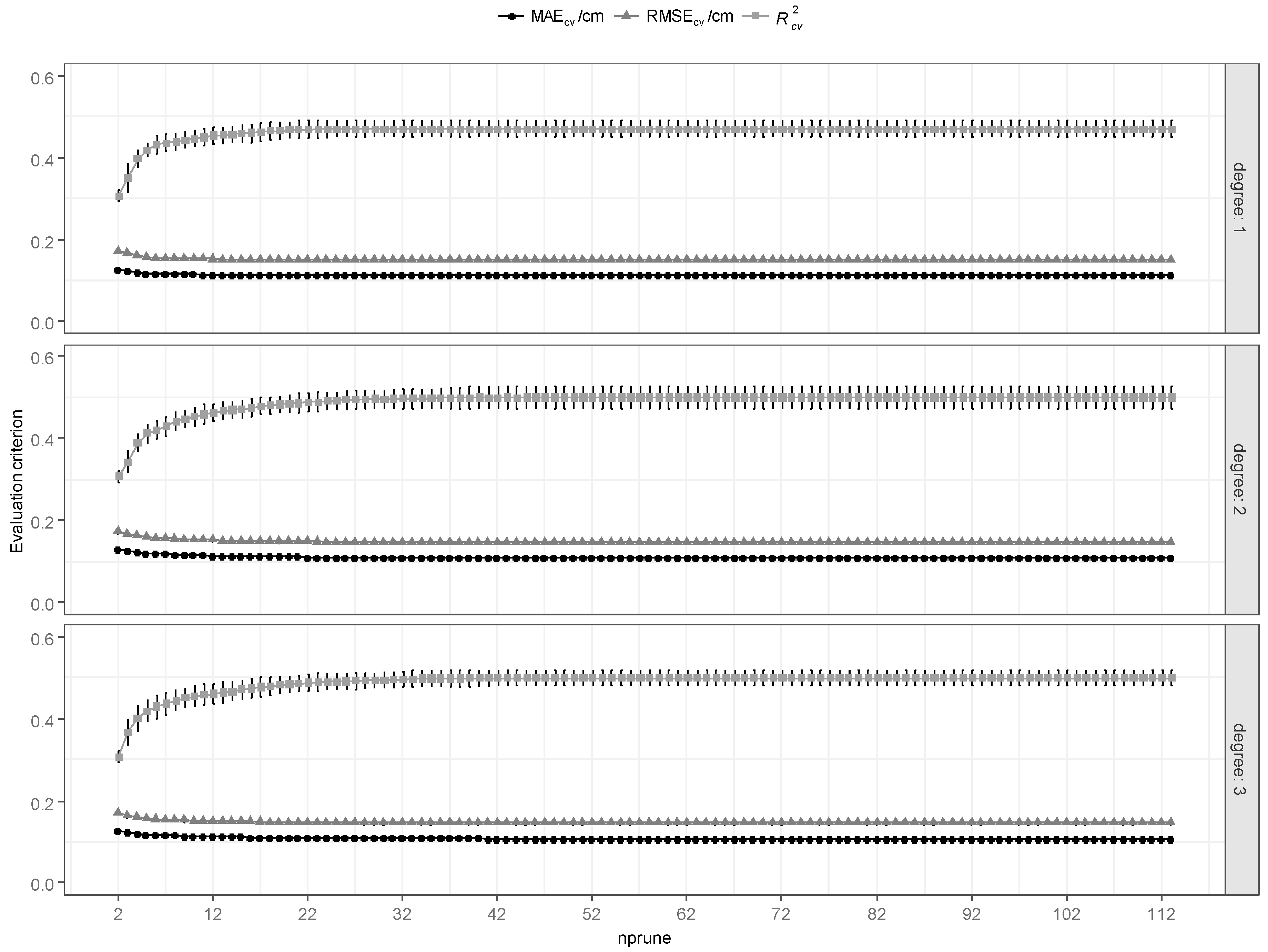
3.1.4. MARS
3.1.5. Model Evaluation and Comparisons
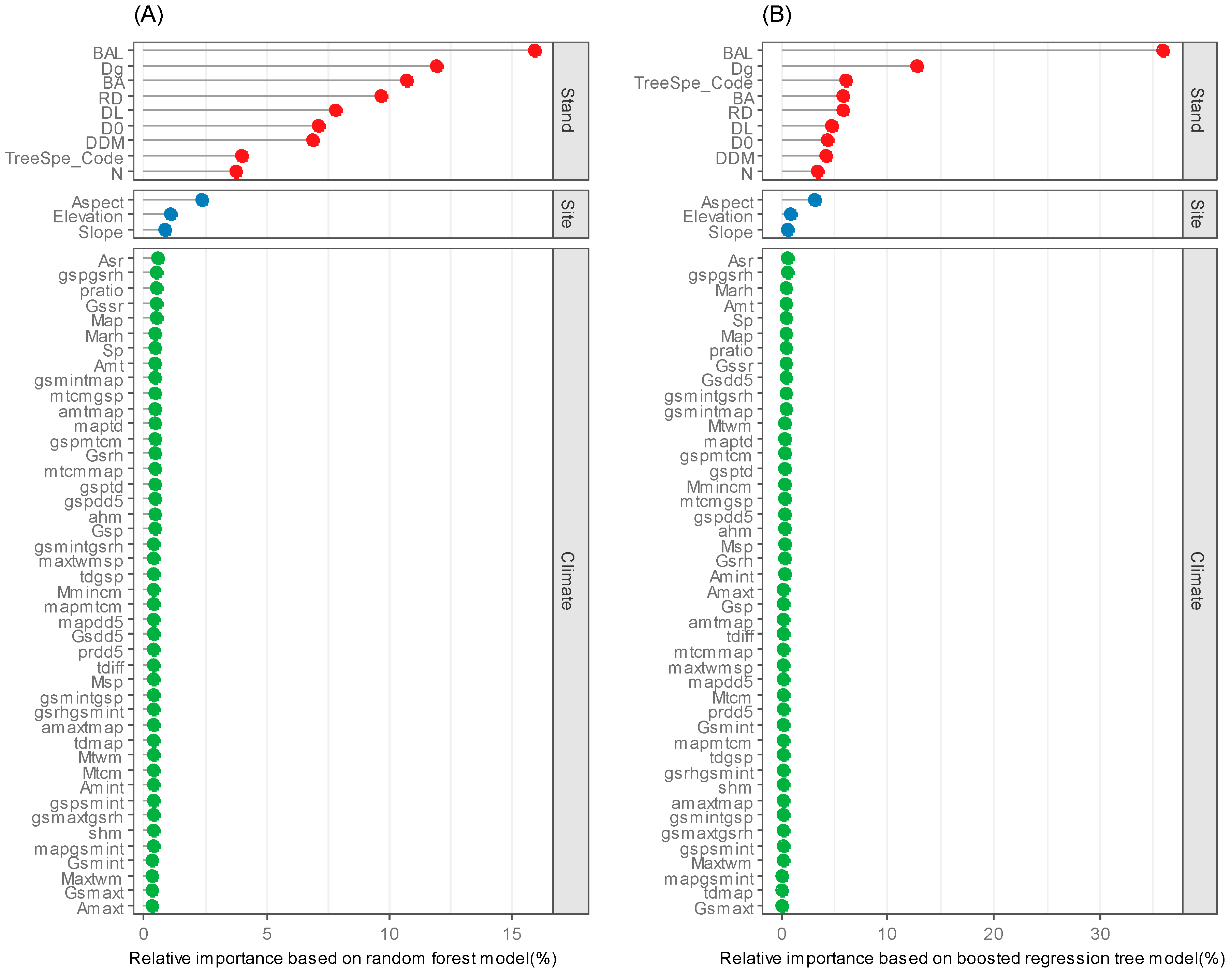
3.2. Variable Importance Based on the Optimal RF and BRT Models
4. Discussion
4.1. ML Model Development
4.2. Performance Evaluations of Four Optimal Models
4.3. Variable Importance in Predicating Individual Tree DBH Growth
5. Conclusions
Author Contributions
Acknowledgments
Conflicts of Interest
References
- Peng, C. Growth and yield models for uneven-aged stands: Past, present and future. For. Ecol. Manag. 2000, 132, 259–279. [Google Scholar] [CrossRef]
- Gyawali, A.; Sharma, R.P.; Bhandari, S.K. Individual tree basal area growth models for Chir pine (Pinus roxberghii Sarg.) in western Nepal. J. For. Sci. 2015, 61, 535–543. [Google Scholar] [CrossRef]
- Porté, A.; Bartelink, H.H. Modelling mixed forest growth: A review of models for forest management. Ecol. Model. 2002, 150, 141–188. [Google Scholar] [CrossRef]
- Ashraf, M.I.; Zhao, Z.; Bourque, C.P.A.; Maclean, D.A.; Meng, F.R. Integrating biophysical controls in forest growth and yield predictions with artificial intelligence technology. Can. J. For. Res. 2013, 43, 1162–1171. [Google Scholar] [CrossRef]
- Ritchie, M.W.; Hann, D.W. Implications of disaggregation in forest growth and yield modeling. For. Sci. 1997, 43, 223–233. [Google Scholar]
- Mabvurira, D.; Miina, J. Individual-tree growth and mortality models for Eucalyptus grandis (Hill) Maiden plantations in Zimbabwe. For. Ecol. Manag. 2002, 161, 231–245. [Google Scholar] [CrossRef]
- Zhao, D.; Borders, B.; Wilson, M. Individual-tree diameter growth and mortality models for bottomland mixed-species hardwood stands in the lower Mississippi alluvial valley. For. Ecol. Manag. 2004, 199, 307–322. [Google Scholar] [CrossRef]
- Biging, G.S.; Dobbertin, M. Evaluation of competition indices in individual tree growth models. For. Sci. 1995, 41, 360–377. [Google Scholar]
- Ma, W.; Lei, X. Nonlinear simultaneous equations for individual-tree diameter growth and mortality model of natural Mongolian oak forests in Northeast China. Forests 2015, 6, 2261–2280. [Google Scholar] [CrossRef]
- Feeley, K.J.; Wright, S.J.; Supardi, M.N.N.; Kassim, A.R.; Davies, S.J. Decelerating growth in tropical forest trees. Ecol. Lett. 2007, 10, 461–469. [Google Scholar] [CrossRef]
- Sánchez-Salguero, R.; Linares, J.C.; Camarero, J.J.; Madrigal-González, J.; Hevia, A.; Sánchez-Miranda, Á.; Ballesteros-Cánovas, J.A.; Alfaro-Sánchez, R.; García-Cervigón, A.I.; Bigler, C. Disentangling the effects of competition and climate on individual tree growth: A retrospective and dynamic approach in Scots pine. For. Ecol. Manag. 2015, 358, 12–25. [Google Scholar] [CrossRef]
- Trasobares, A.; Zingg, A.; Walthert, L.; Bigler, C. A climate-sensitive empirical growth and yield model for forest management planning of even-aged beech stands. Eur. J. For. Res. 2016, 135, 263–282. [Google Scholar] [CrossRef]
- Zang, H.; Lei, X.; Ma, W.; Zeng, W. Spatial heterogeneity of climate change effects on dominant height of larch plantations in northern and northeastern China. Forests 2016, 7, 151. [Google Scholar] [CrossRef]
- Jiang, X.; Huang, J.G.; Cheng, J.; Dawson, A.; Stadt, K.J.; Comeau, P.G.; Chen, H.Y.H. Interspecific variation in growth responses to tree size, competition and climate of western Canadian boreal mixed forests. Sci. Total Environ. 2018, 631, 1070–1078. [Google Scholar] [CrossRef] [PubMed]
- Subedi, N.; Sharma, M. Climate-diameter growth relationships of black spruce and jack pine trees in boreal Ontario, Canada. Glob. Chang. Biol. 2013, 19, 505–516. [Google Scholar] [CrossRef] [PubMed]
- Chen, L.; Huang, J.G.; Stadt, K.J.; Comeau, P.G.; Zhai, L.; Dawson, A.; Alam, S.A. Drought explains variation in the radial growth of white spruce in western Canada. Agric. Forest Meteorol. 2017, 233, 133–142. [Google Scholar] [CrossRef]
- Cortini, F.; Filipescu, C.N.; Groot, A.; MacIsaac, D.A.; Nunifu, T. Regional models of diameter as a function of individual tree attributes, climate and site characteristics for six major tree species in Alberta, Canada. Forests 2011, 2, 814–831. [Google Scholar] [CrossRef]
- Toledo, M.; Poorter, L.; Peña-Claros, M.; Alarcón, A.; Balcázar, J.; Leaño, C.; Licona, J.C.; Llanque, O.; Vroomans, V.; Zuidema, P. Climate is a stronger driver of tree and forest growth rates than soil and disturbance. J. Ecol. 2011, 99, 254–264. [Google Scholar] [CrossRef]
- Yu, L.; Lei, X.; Wang, Y.; Yang, Y.; Wang, Q. Impact of climate on individual tree radial growth based on generalized additive model. J. Beijing For. Univ. 2014, 36, 22–32, (In Chinese with English abstract). [Google Scholar]
- Vieira, G.C.; de Mendonça, A.R.; da Silva, G.F.; Zanetti, S.S.; da Silva, M.M.; dos Santos, A.R. Prognoses of diameter and height of trees of eucalyptus using artificial intelligence. Sci. Total Environ. 2018, 619–620, 1473–1481. [Google Scholar] [CrossRef]
- De’Ath, G. Boosted trees for ecological modeling and prediction. Ecology 2007, 88, 243–251. [Google Scholar] [CrossRef]
- Yang, R.; Zhang, G.; Liu, F.; Lu, Y.; Yang, F.; Yang, F.; Yang, M.; Zhao, Y.; Li, D. Comparison of boosted regression tree and random forest models for mapping topsoil organic carbon concentration in an alpine ecosystem. Ecol. Indic. 2016, 60, 870–878. [Google Scholar] [CrossRef]
- Tramontana, G.; Ichii, K.; Camps-Valls, G.; Tomelleri, E.; Papale, D. Uncertainty analysis of gross primary production upscaling using Random Forests, remote sensing and eddy covariance data. Remote. Sens. Environ. 2015, 168, 360–373. [Google Scholar] [CrossRef]
- Papale, D.; Black, T.A.; Carvalhais, N.; Cescatti, A.; Chen, J.; Jung, M.; Kiely, G.; Lasslop, G.; Mahecha, M.D.; Margolis, H.; et al. Effect of spatial sampling from European flux towers for estimating carbon and water fluxes with artificial neural networks. J. Geophys. Res. Biogeosci. 2015, 120, 1941–1957. [Google Scholar] [CrossRef]
- Périé, C.; de Blois, S. Dominant forest tree species are potentially vulnerable to climate change over large portions of their range even at high latitudes. Peer J. 2016, 4, e2218. [Google Scholar] [CrossRef] [PubMed]
- Pouteau, R.; Meyer, J.Y.; Taputuarai, R.; Stoll, B. Support vector machines to map rare and endangered native plants in Pacific islands forests. Ecol. Inform. 2012, 9, 37–46. [Google Scholar] [CrossRef]
- Kuhn, M.; Johnson, K. Applied Predictive Modeling; Springer: New York, NY, USA, 2013. [Google Scholar]
- Prasad, A.M.; Iverson, L.R.; Liaw, A. Newer classification and regression tree techniques: Bagging and random forests for ecological prediction. Ecosystems 2006, 9, 181–199. [Google Scholar] [CrossRef]
- Shen, C. Climate-Sensitive Site Index Model of Larix olgensis Henry. Master’s Thesis, Chinese Academy of Forestry, Beijing, China, 2012. (In Chinese). [Google Scholar]
- Breiman, L. Random Forest. Mach. Learn. 2001, 45, 5–32. [Google Scholar] [CrossRef]
- Liaw, A.; Wiener, M. Classification and Regression by random Forest. R. News 2002, 2, 18–22. [Google Scholar]
- R Development Core Team. R: A Language and Environment for Statistical Computing; R Foundation for Statistical Computing: Vienna, Austria, 2015; Available online: http://www.r-project.org (accessed on 21 April 2017).
- Freeman, E.A.; Moisen, G.G.; Coulston, J.W.; Wilson, B.T. Random forests and stochastic gradient boosting for predicting tree canopy cover: Comparing tuning processes and model performance1. Can. J. For. Res. 2016, 46, 323–339. [Google Scholar] [CrossRef]
- Zhang, R.; Pang, Y.; Li, Z.; Bao, Y. Canopy closure estimation in a temperate forest using airborne LiDAR and LANDSAT ETM+ data. Chin. J. Plant Ecol. 2016, 40, 102–115, (In Chinese with English abstract). [Google Scholar]
- Kuhn, M. Classification and Regression Training. Available online: https://cran.r-project.org/web/packages/caret/caret.pdf (accessed on 20 November 2018).
- Mansiaux, Y.; Carrat, F. Detection of independent associations in a large epidemiologic dataset: A comparison of random forests, boosted regression trees, conventional and penalized logistic regression for identifying independent factors associated with H1N1pdm influenza infection. BMC Med. Res. Methodol. 2014, 14, 9. [Google Scholar] [CrossRef] [PubMed]
- Friedman, J.H. Stochastic gradient boosting. Comput. Stat. Data Anal. 2002, 38, 367–378. [Google Scholar] [CrossRef]
- Ridgeway, G. Generalized Boosted Models: A Guide to the gbm Package. Available online: https://cran.r-project.org/web/packages/gbm/vignettes/gbm.pdf (accessed on 14 September 2018).
- Elith, J.; Leathwick, J.R.; Hastie, T. A working guide to boosted regression trees. J. Anim. Ecol. 2008, 77, 802–813. [Google Scholar] [CrossRef] [PubMed]
- Kuhn, M.; Weston, S.; Keefer, C.; Coulter, N.; Quinlan, R.; Rulequest Research Pty Ltd. Rule- and Instance-Based Regression Modeling. Available online: https://cran.r-project.org/web/packages/Cubist/Cubist.pdf (accessed on 21 May 2018).
- Sun, B.; Lam, D.; Yang, D.; Grantham, K.; Zhang, T.; Mutic, S.; Zhao, T. A machine learning approach to the accurate prediction of monitor units for a compact proton machine. Med. Phys. 2018, 45, 2243–2251. [Google Scholar] [CrossRef] [PubMed]
- Ferlito, S.; Adinolfi, G.; Graditi, G. Comparative analysis of data-driven methods online and offline trained to the forecasting of grid-connected photovoltaic plant production. Appl. Energy 2017, 205, 116–129. [Google Scholar] [CrossRef]
- Friedman, J.H. Multivariate adaptive regression splines. Ann. Stat. 1991, 19, 1–67. [Google Scholar] [CrossRef]
- Lee, T.S.; Chiu, C.C.; Chou, Y.C.; Lu, C.J. Mining the customer credit using classification and regression tree and multivariate adaptive regression splines. Comput. Stat. Data Anal. 2006, 50, 1113–1130. [Google Scholar] [CrossRef]
- Heddam, S.; Kisi, O. Modelling daily dissolved oxygen concentration using least square support vector machine, multivariate adaptive regression splines and M5 model tree. J. Hydrol. 2018, 559, 499–509. [Google Scholar] [CrossRef]
- Milborrow, S. Multivariate Adaptive Regression Splines. Available online: https://cran.r-project.org/web/packages/earth/earth.pdf (accessed on 3 January 2019).
- Hastie, T.; Tibshirani, R.; Friedman, J. The Elements of Statistical Learning: Data Mining, Inference and Prediction, 2nd ed.; Springer: New York, NY, USA, 2009. [Google Scholar]
- Smoliński, S.; Radtke, K. Spatial prediction of demersal fish diversity in the Baltic Sea: Comparison of machine learning and regression-based techniques. ICES J. Mar. Sci. 2017, 74, 102–111. [Google Scholar] [CrossRef]
- Zhou, Z. Machine Learning; Tsinghua University Press: Beijing, China, 2016. (In Chinese) [Google Scholar]
- Breiman, L. Statistical modeling: The two cultures. Stat. Sci. 2001, 16, 199–231. [Google Scholar] [CrossRef]
- Moisen, G.G.; Frescino, T.S. Comparing five modelling techniques for predicting forest characteristics. Ecol. Model. 2002, 157, 209–225. [Google Scholar] [CrossRef]
- Aertsen, W.; Kint, V.; Orshoven, J.V.; Özkan, K.; Muys, B. Comparison and ranking of different modelling techniques for prediction of site index in Mediterranean mountain forests. Ecol. Model. 2010, 221, 1119–1130. [Google Scholar] [CrossRef]
- Leathwick, J.R.; Elith, J.; Francis, M.P.; Hastie, T.; Taylor, P. Variation in demersal fish species richness in the oceans surrounding New Zealand: An analysis using boosted regression trees. Mar. Ecol. Prog. Ser. 2006, 321, 267–281. [Google Scholar] [CrossRef]
- Adame, P.; Hynynen, J.; Cañellas, I.; del Río, M. Individual-tree diameter growth model for rebollo oak (Quercus pyrenaica Willd.) coppices. For. Ecol. Manag. 2008, 255, 1011–1022. [Google Scholar] [CrossRef]
- Lhotka, J.M.; Loewenstein, E.F. An individual-tree diameter growth model for managed uneven-aged oak-shortleaf pine stands in the Ozark Highlands of Missouri, USA. For. Ecol. Manag. 2011, 261, 770–778. [Google Scholar] [CrossRef]
- Alam, S.A.; Huang, J.G.; Stadt, K.J.; Comeau, P.G.; Dawson, A.; Geaizquierdo, G.; Aakala, T.; Hölttä, T.; Vesala, T.; Mäkelä, A.; et al. Effects of competition, drought stress and photosynthetic productivity on the radial growth of white Spruce in Western Canada. Front. Plant Sci. 2017, 8, 1915. [Google Scholar] [CrossRef]
- Lo, Y.H.; Blanco, J.A.; Seely, B.; Welham, C.; Kimmins, J.P. Relationships between climate and tree radial growth in interior British Columbia, Canada. For. Ecol. Manag. 2010, 259, 932–942. [Google Scholar] [CrossRef]


| Variable | Mean | Sd | Minimum | Maximum | Description |
|---|---|---|---|---|---|
| ΔD (cm) | 0.28 | 0.21 | 0 | 2.04 | Individual tree mean annual DBH increment within an interval of any five consecutive years |
| N (trees·hm−2) | 1017 | 245 | 395 | 1585 | The number of trees per hectare |
| BA (m2·hm−2) | 26.26 | 5.42 | 14.22 | 37.37 | Basal area per hectare |
| Dg (cm) | 18.31 | 2.13 | 13.01 | 22.95 | Average DBH |
| Slope (°) | 9.25 | 3.54 | 6.00 | 18.00 | Slope |
| Elevation (m) | 691.10 | 62.79 | 600.00 | 800.00 | Elevation |
| Type | Variables | Description | Variables | Description |
|---|---|---|---|---|
| Temperature | Amaxt (°C) | Annual maximum temperature | Amint (°C) | Annual minimum temperature |
| Amt (°C) | Annual mean temperature | Gsdd5 (°C) | The accumulated temperature is greater than 5 °C in growing season (April–September) | |
| Gsmaxt (°C) | Maximum temperature in growing season (April–September) | Gsmint (°C) | Minimum temperature in growing season (4–9 months) | |
| Maxtwm (°C) | The highest temperature in the hottest month (July) | Mmincm (°C) | The lowest temperature of the coldest month (January) | |
| Mtcm (°C) | The mean temperature of the coldest month (January) | Mtwm (°C) | The mean temperature of the hottest month (July) | |
| Precipitation | Gsp (mm) | Average precipitation in growing season (April–September) | Map (mm) | Annual mean precipitation |
| Msp (mm) | Monthly total precipitation | Sp (mm) | Summer precipitation (June–August) | |
| Gsrh (%) | Relative humidity in growing season (April–September) | Marh (%) | Annual mean relative humidity | |
| Illumination | Asr (h) | Annual total solar radiation duration | Gssr (h) | Solar radiation duration in growing season (April–September) |
| Composite climatic factors generated by the interaction of basic climatic factors | ahm (°C·mm−1) | 1000 × ((Amt + 10)/Map) | shm (°C) | Gsmaxt + Maxtwm |
| amaxtmap (°C·mm−1) | Amaxt/Map | amtmap (°C·mm−1) | Amt/Map | |
| gsmaxtgsrh (100 °C) | (Gsmaxt × Gsrh)/1000 | gsmintgsp (°C·mm−1) | Gsmint/Gsp | |
| gsmintgsrh (100 °C) | Gsmint/Gsrh | gsmintmap (°C·mm−1) | Gsmint/Map | |
| gspdd5 (mm·°C) | (Gsp × Gsdd5)/1000 | gspgsrh (100 mm) | Gsp/Gsrh | |
| gspmtcm (mm·°C) | (Gsp × Mtcm)/1000 | gspgsmint (mm·°C) | (Gsp × Gsmint)/1000 | |
| gsrhgsmint (100 °C) | (Gsrh × Gsmint)/1000 | mapdd5 (mm·°C) | (Map × Gsdd5)/1000 | |
| mapgsmint (mm·°C) | (Map × Gsmint)/1000 | mapmtcm (mm·°C) | (Map × Mtcm)/1000 | |
| maxtwmsp (°C·mm−1) | Maxtwm/Sp | mtcmgsp (°C·mm−1) | Mtcm/Gsp | |
| mtcmmap (°C·mm−1) | Mtcm/Map | pratio | Gsp/Map | |
| prdd5 (°C) | pratio × Gsdd5 | tdiff (°C) | Mtwm − Mtcm | |
| tdgsp (°C·mm−1) | tdiff/Gsp | gsptd (°C·mm) | (Gsp × tdiff)/1000 | |
| maptd (°C·mm) | (Map × tdiff)/1000 | tdmap (°C·mm−1) | tdiff/Map |
| Evaluation Criteria | Models | |||
|---|---|---|---|---|
| RF | BRT | Cubist | MARS | |
| R2cv | 0.5565(0.0186) a | 0.5711(0.0232) a | 0.5734(0.0215) a | 0.4993(0.0262) b |
| RMSEcv (cm) | 0.1377(0.0044) b | 0.1353(0.0050) b | 0.1351(0.0048) b | 0.1462(0.0047) a |
| MAEcv (cm) | 0.0996(0.0015) b | 0.0985(0.0018) bc | 0.0972(0.0015) c | 0.1086(0.0022) a |
© 2019 by the authors. Licensee MDPI, Basel, Switzerland. This article is an open access article distributed under the terms and conditions of the Creative Commons Attribution (CC BY) license (http://creativecommons.org/licenses/by/4.0/).
Share and Cite
Ou, Q.; Lei, X.; Shen, C. Individual Tree Diameter Growth Models of Larch–Spruce–Fir Mixed Forests Based on Machine Learning Algorithms. Forests 2019, 10, 187. https://doi.org/10.3390/f10020187
Ou Q, Lei X, Shen C. Individual Tree Diameter Growth Models of Larch–Spruce–Fir Mixed Forests Based on Machine Learning Algorithms. Forests. 2019; 10(2):187. https://doi.org/10.3390/f10020187
Chicago/Turabian StyleOu, Qiangxin, Xiangdong Lei, and Chenchen Shen. 2019. "Individual Tree Diameter Growth Models of Larch–Spruce–Fir Mixed Forests Based on Machine Learning Algorithms" Forests 10, no. 2: 187. https://doi.org/10.3390/f10020187
APA StyleOu, Q., Lei, X., & Shen, C. (2019). Individual Tree Diameter Growth Models of Larch–Spruce–Fir Mixed Forests Based on Machine Learning Algorithms. Forests, 10(2), 187. https://doi.org/10.3390/f10020187