Spatial Analysis of Temperate Forest Structure: A Geostatistical Approach to Natural Forest Potential


 , , ,
, , ,  and
and
Abstract
1. Introduction
2. Materials and Methods
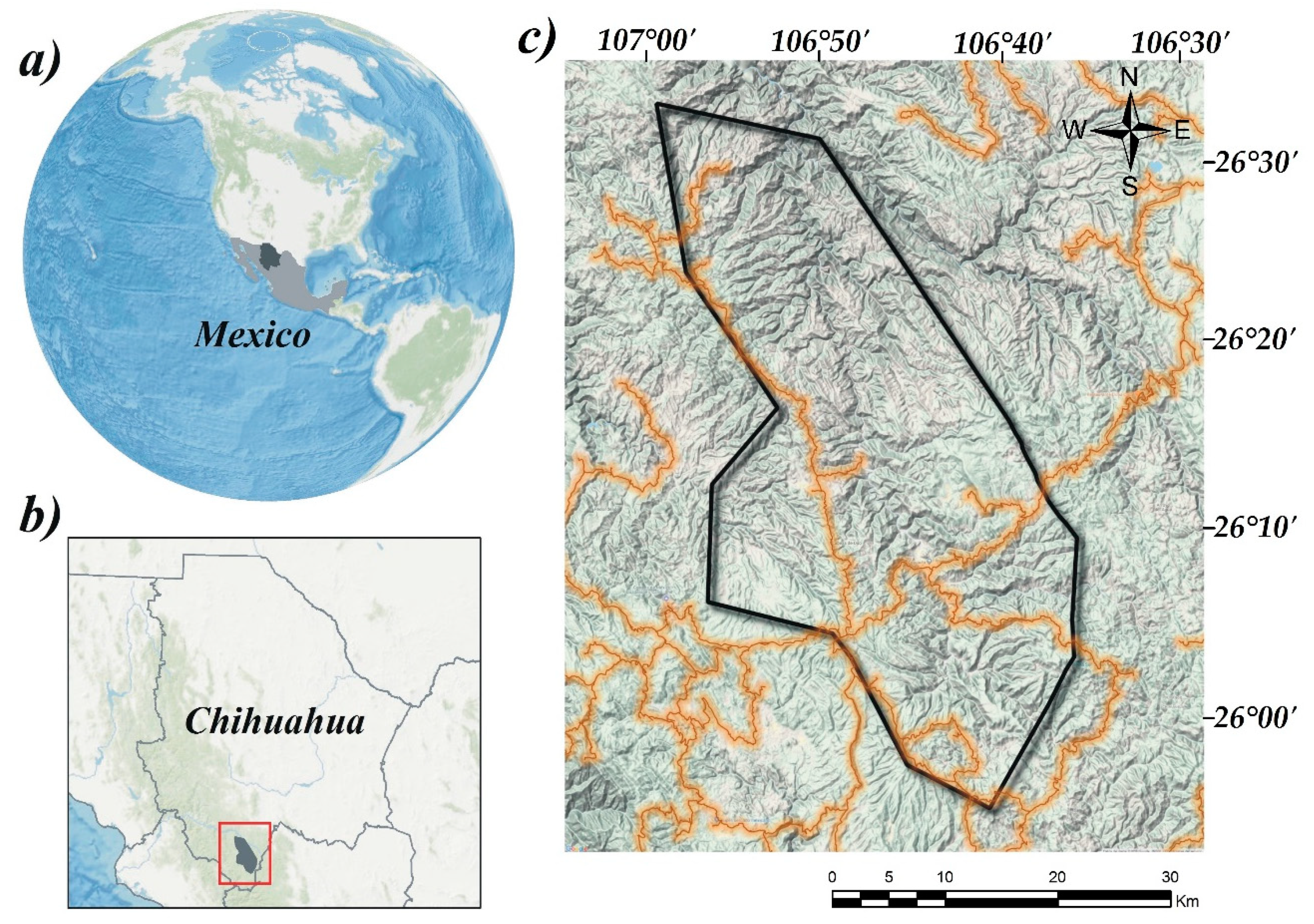
2.1. Study Area
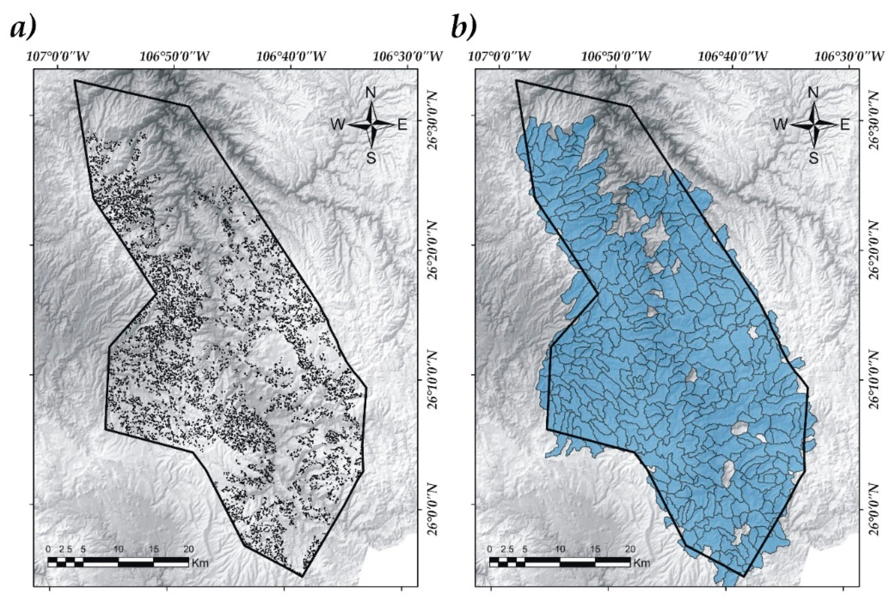
2.2. Forest Data
2.3. Geospatial Data
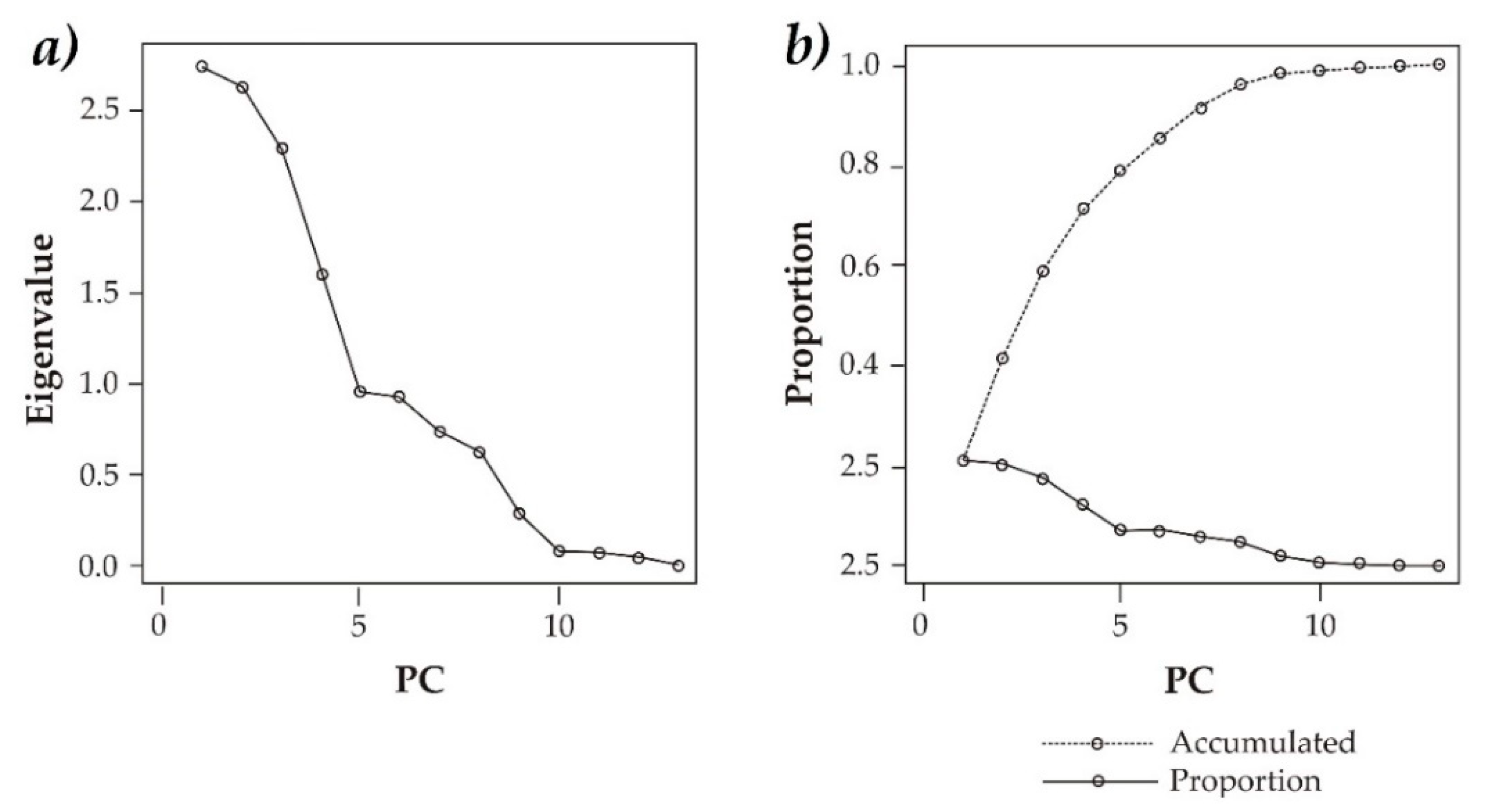
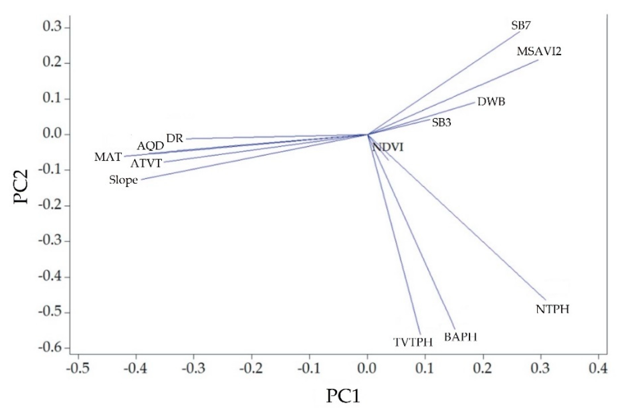
2.4. Statistical Analyses
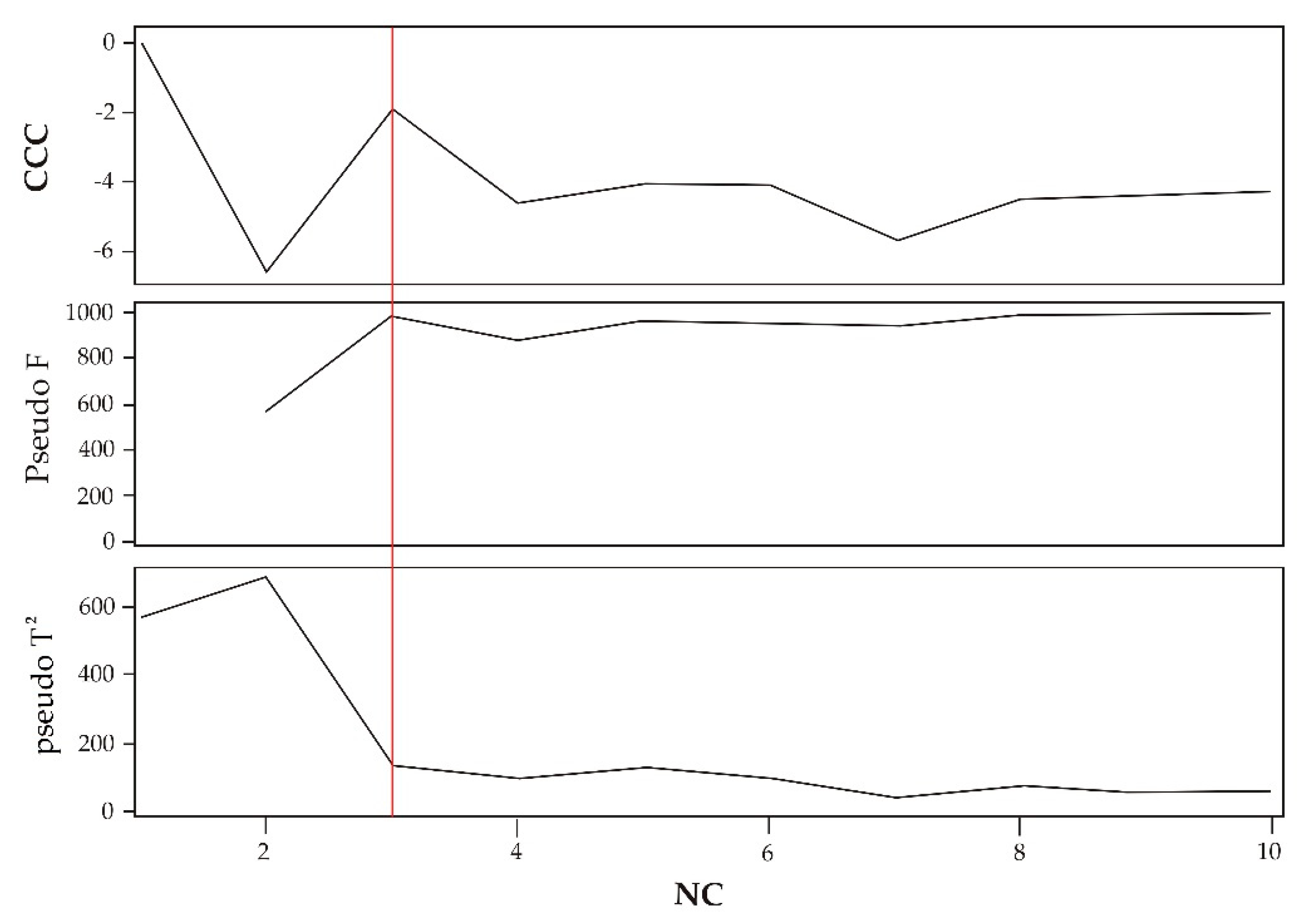
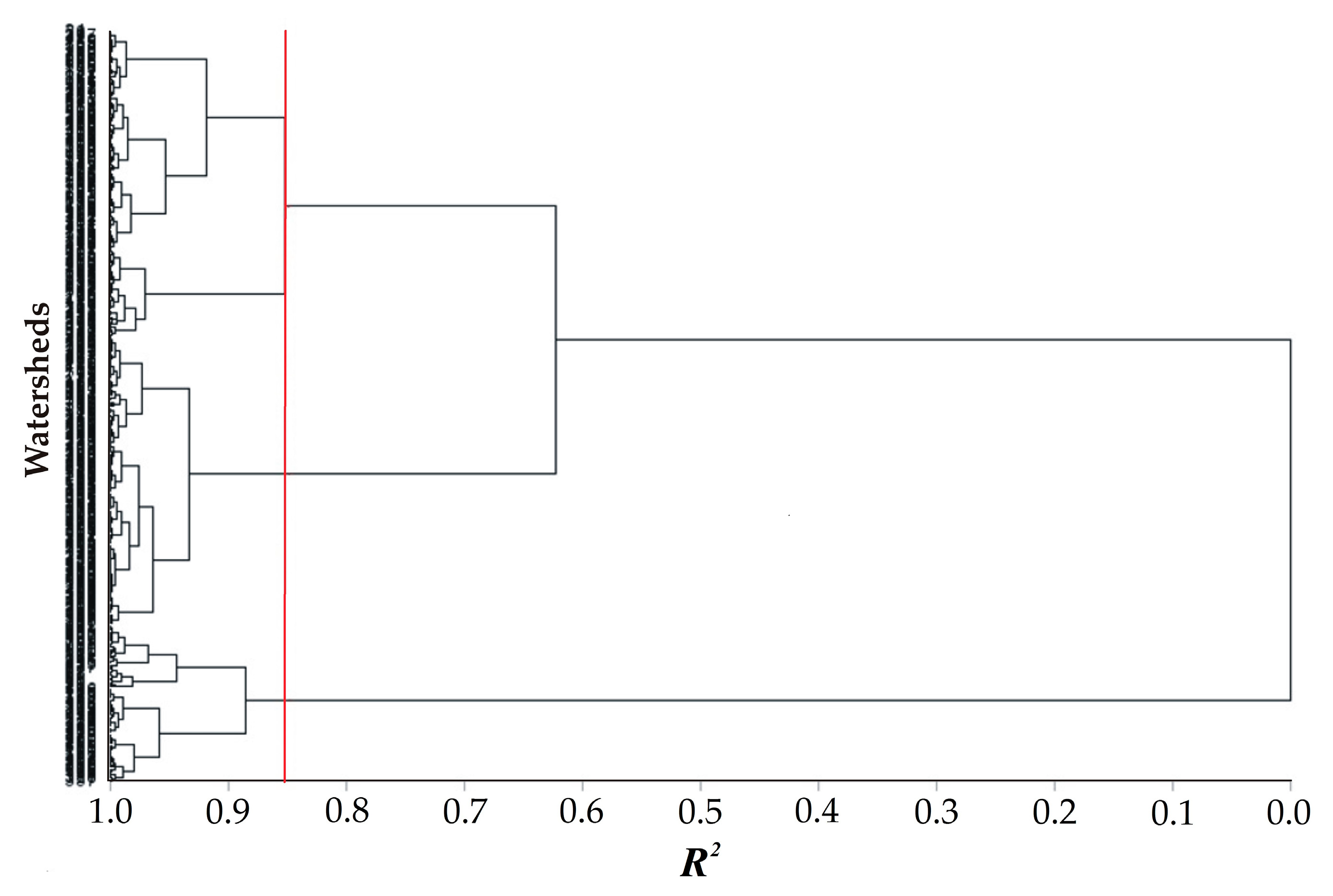
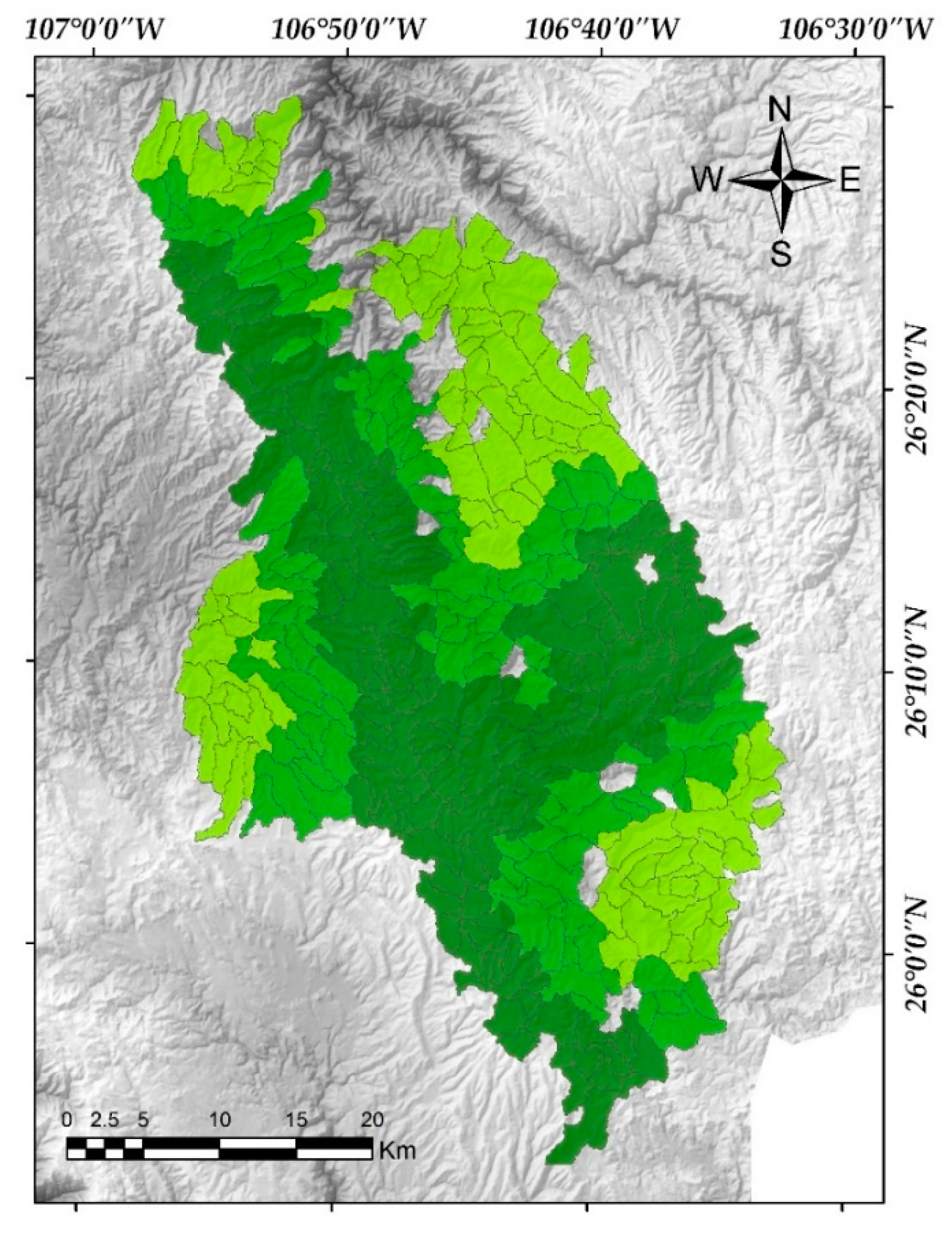
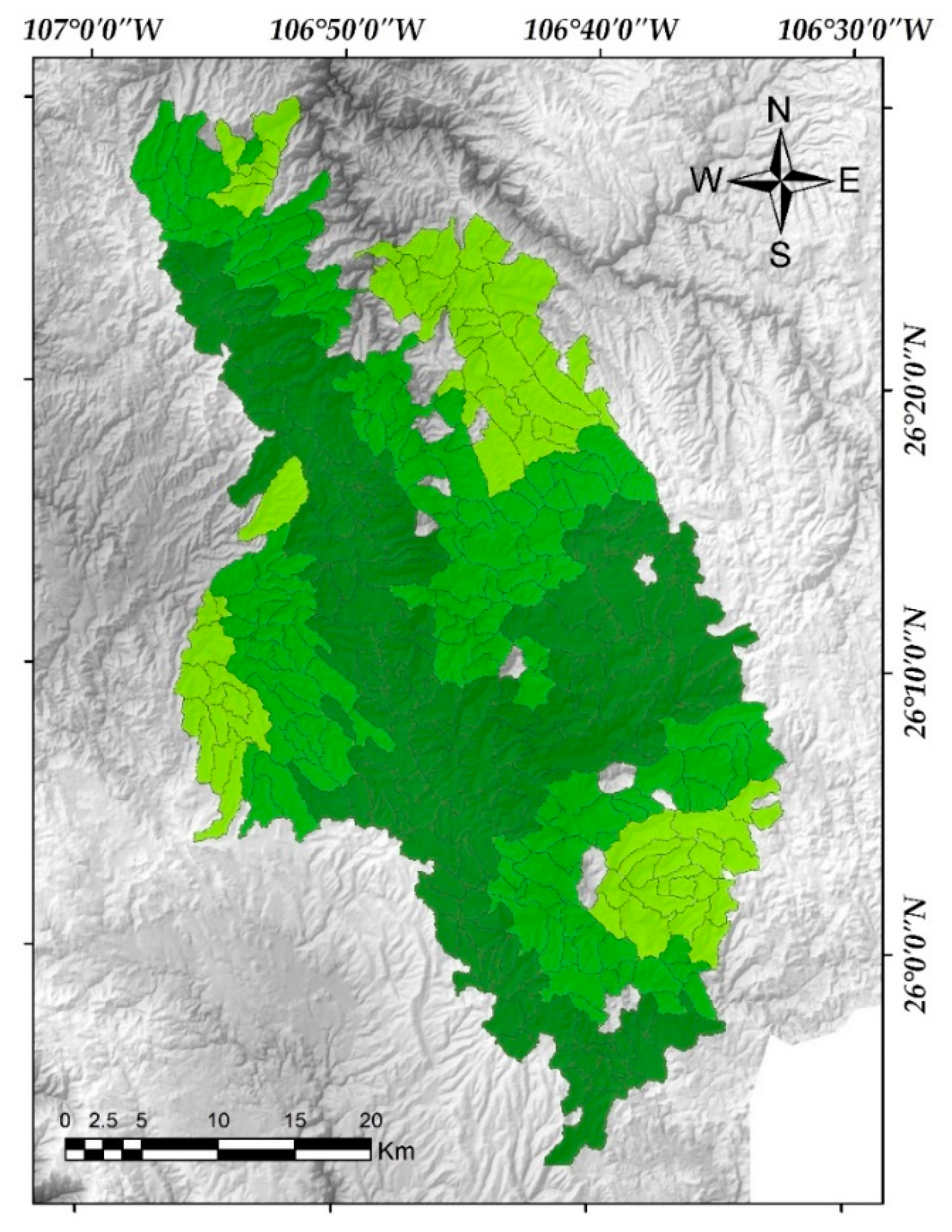
3. Results
4. Discussion
5. Conclusions
Author Contributions
Acknowledgments
Conflicts of Interest
References
- Randolph, J.C.; Green, G.M.; Belmont, J.; Burcsu, T.; Welch, D. Forest Ecosystems and the Human Dimension. In Seeing the Forest and the Trees: Human–Environment Interactions in Forest Ecosystems; Moran, E.F., Ostrom, E., Eds.; MIT Press: Cambridge, MA, USA, 2005; pp. 81–103. [Google Scholar]
- Bolton, D.K.; Coops, N.C.; Hermosillo, T.; Wulder, M.A.; White, J.C. Assessing variability in postfire forest structure along gradients of productivity in the Canadian boreal using multisource remote sensing. J. Biogeogr. 2017, 44, 1294–1305. [Google Scholar] [CrossRef]
- Hilker, T.; Wulder, M.A.; Coops, N.C.; Linke, J.; McDermid, G.; Masek, J.G.; Gao, F.; White, J.C. A new data fusion model for high spatial-and temporal-resolution mapping of forest disturbance based on Landsat and MODIS. Remote Sens. Environ. 2009, 113, 1613–1627. [Google Scholar] [CrossRef]
- Sáenz, R.C.; Rehfeldt, G.E.; Crookston, N.L.; Duval, P.; Amant, R.S.T.; Beaulieu, J.B.; Richardson, A. Spline models of contemporary, 2030, 2060 and 2090 climates for Mexico and their use in understanding climate-change impacts on the vegetation. Clim. Chang. 2010, 102, 595–623. [Google Scholar] [CrossRef]
- Groombridge, B.; Jenkins, M.D. Global Biodiversity: Earth’s Living Resources in the 21st Century; World Conservation Press: Cambridge, MA, USA, 2000. [Google Scholar]
- González, E.M.; Meave, J.A.; Marcial, N.R.; Aceves, T.T.; Hernández, F.G.; Manríquez, G.I. Los bosques de niebla de México: conservación y restauración de su componente arbóreo. Rev. Ecosistemas 2012, 21, 1–2. [Google Scholar]
- Challenger, A. La zona ecológica templada húmeda. In Utilización y Conservación de Los Ecosistemas Terrestres de México: Pasado, Presente y Futuro; CONABIO-Instituto de Biología, UNAM Sierra Madre: Mexico City, México, 1998; pp. 433–518. [Google Scholar]
- Velázquez, A.; Mas, J.F.; Gallegos, J.R.D.; Saucedo, R.M.; Alcántara, P.C.; Castro, R.; Palacio, J.L. Patrones y tasas de cambio de uso del suelo en México. Gaceta Ecológica 2002, 62. Available online: https://www.redalyc.org/articulo.oa?id=53906202 (accessed on 18 January 2019).
- Aguilar, S.V.; Castillo, M.A.; Guerrero, V.F.; Wehenkel, C.; Pinedo, A.C. Modeling the potential distribution of Picea chihuahuana Martínez, an endangered species at the Sierra Madre Occidental, Mexico. Forest 2015, 6, 692–707. [Google Scholar] [CrossRef]
- Jupp, D.L.; Walker, J. Detecting structural and growth changes in woodlands and forests: The challenge for remote sensing and the role of geometric-optical modelling. In The Use of Remote Sensing in the Modeling of Forest Productivity; Springer: Dordrecht, Netherlands, 1997; pp. 75–108. [Google Scholar]
- Ludwig, B.; Khanna, P.K.; Raison, R.J.; Jacobsen, K. Modelling changes in cation composition of a soil after clearfelling a eucalypt forest in East Gippsland, Australia. Geoderma 1997, 80, 95–116. [Google Scholar] [CrossRef]
- Achard, F.; Mollicone, D.; Stibig, H.J.; Aksenov, D.; Laestadius, L.; Li, Z.; Potapov, P.; Yaroshenko, A. Areas of rapid forest-cover change in boreal Eurasia. For. Ecol. Manag. 2006, 237, 322–334. [Google Scholar] [CrossRef]
- Bonan, G.B. Forests and climate change: forcing, feedbacks, and the climate benefits of forests. Science. 2008, 320, 1444–1449. [Google Scholar] [CrossRef]
- Chambers, J.Q.; Asner, G.P.; Morton, D.C.; Anderson, L.O.; Saatchi, S.S.; Espírito-Santo, F.D.; Souza, C. Regional ecosystem structure and function: ecological insights from remote sensing of tropical forests. Trends Ecol. Evol. 2007, 22, 414–423. [Google Scholar] [CrossRef]
- Zhu, Z.; Woodcock, C.E.; Olofsson, P. Continuous monitoring of forest disturbance using all available Landsat imagery. Remote Sens. Environ. 2012, 122, 75–91. [Google Scholar] [CrossRef]
- Franklin, S.E. Remote sensing for sustainable forest management; CRC Press: Boca Raton, FL, USA, 2001. [Google Scholar]
- Wang, X.; Shao, G.; Chen, H.; Lewis, B.J.; Qi, G.; Yu, D.; Dai, L. An Application of remote sensing data in mapping landscape-level forest biomass for monitoring the effectiveness of forest policies in Northeastern China. Environ. Manag. 2013, 52, 612–620. [Google Scholar] [CrossRef]
- Pflugmacher, D.; Cohen, W.B.; Kennedy, R.E. Using Landsat-derived disturbance history (1972–2010) to predict current forest structure. Remote Sens. Environ. 2012, 122, 146–165. [Google Scholar] [CrossRef]
- Ingram, J.C.; Dawson, T.P.; Whittaker, R.J. Mapping tropical forest structure in southeastern Madagascar using remote sensing and artificial neural networks. Remote Sens. Environ. 2005, 94, 491–507. [Google Scholar] [CrossRef]
- Powell, S.L.; Cohen, W.B.; Healey, S.P.; Kennedy, R.E.; Moisen, G.G.; Pierce, K.B.; Ohmann, J.L. Quantification of live aboveground forest biomass dynamics with Landsat time-series and field inventory data: A comparison of empirical modeling approaches. Remote Sens. Environ. 2010, 114, 1053–1068. [Google Scholar] [CrossRef]
- Wolter, P.T.; Townsend, P.A.; Sturtevant, B.R. Estimation of forest structural parameters using 5 and 10 meter SPOT-5 satellite data. Remote Sens. Environ. 2009, 113, 2019–2036. [Google Scholar] [CrossRef]
- Dube, T.; Mutanga, O. Evaluating the utility of the medium-spatial resolution Landsat 8 multispectral sensor in quantifying aboveground biomass in uMgeni catchment, South Africa. ISPRS J. Photogramm. 2015, 101, 36–46. [Google Scholar] [CrossRef]
- Soenen, S.A.; Peddle, D.R.; Hall, R.J.; Coburn, C.A.; Hall, F.G. Estimating aboveground forest biomass from canopy reflectance model inversion in mountainous terrain. Remote Sens. Environ. 2010, 114, 1325–1337. [Google Scholar] [CrossRef]
- Bach, K.; Schawe, M.; Beck, S.; Gerold, G.; Gradstein, S.R.; Moraes, R. Vegetación, suelos y clima en los diferentes pisos altitudinales de un bosque montano de Yungas, Bolivia: Primeros resultados. Ecología en Bolivia 2003, 38, 3–14. [Google Scholar]
- Sanderson, M.; Santini, M.; Valentini, R.; Pope, E. Relationships between forests and weather. EC Directorate General of the Environment; Met Office: Devon, UK, 2012. Available online: http://ec.europa.eu/environment/forests/pdf/EU_Forests_annex1.pdf (accessed on 19 October 2018).
- Vázquez-Quintero, G.; Solís-Moreno, R.; Pompa-García, M.; Villarreal-Guerrero, F.; Pinedo-Alvarez, C.; Pinedo-Alvarez, A. Detection and projection of forest changes by using the Markov Chain Model and Cellular Automata. Sustainability 2016, 8, 236. [Google Scholar] [CrossRef]
- Pasher, J.; King, D.J. Multivariate forest structure modelling and mapping using high resolution airborne imagery and topographic information. Remote Sens. Environ. 2010, 114, 1718–1732. [Google Scholar] [CrossRef]
- Bhuiyan, M.A.; Rakib, M.A.; Dampare, S.B.; Ganyaglo, S.; Suzuki, S. Surface water quality assessment in the central part of Bangladesh using multivariate analysis. Ksce J. Civ. Eng. 2011, 15, 995–1003. [Google Scholar] [CrossRef]
- Batayneh, A.; Zumlot, T. Multivariate statistical approach to geochemical methods in water quality factor identification; application to the shallow aquifer system of the Yarmouk basin of north Jordan. Res. J. Environ. Earth Sci. 2012, 4, 756–768. [Google Scholar]
- Oketola, A.A.; Adekolurejo, S.M.; Osibanjo, O. Water quality assessment of River Ogun using multivariate statistical techniques. J. Environ. Prot. Ecol. 2013, 4, 466. [Google Scholar] [CrossRef]
- Singh, K.P.; Malik, A.; Mohan, D.; Sinha, S. Multivariate statistical techniques for the evaluation of spatial and temporal variations in water quality of Gomti River (India)—A case study. Water Res. 2004, 38, 3980–3992. [Google Scholar] [CrossRef]
- Kalabokidis, K.D.; Koutsias, N.; Konstantinidis, P.; Vasilakos, C. Multivariate analysis of landscape wildfire dynamics in a Mediterranean ecosystem of Greece. Area 2007, 39, 392–402. [Google Scholar] [CrossRef]
- Verdú, F.; Salas, J.; García, C.V. A multivariate analysis of biophysical factors and forest fires in Spain, 1991–2005. Int J. Wildland Fire 2012, 21, 498–509. [Google Scholar] [CrossRef]
- Tritsch, I.; Sist, P.; Narvaes, I.D.S.; Mazzei, L.; Blanc, L.; Bourgoin, C.; Gond, V. Multiple patterns of forest disturbance and logging shape forest landscapes in Paragominas, Brazil. Forests 2016, 7, 315. [Google Scholar] [CrossRef]
- Torres, A.B.; Acuña, L.; Vergara, J.M. Integrating CBM into land-use based mitigation actions implemented by local communities. Forests 2014, 5, 3295–3326. [Google Scholar] [CrossRef]
- Felger, R.S.; Johnson, M.B. Trees of the northern Sierra Madre Occidental and sky islands of southwestern North America. In Biodiversity and Management of the Madrean archipelago: The Sky Islands of Southwestern United States and Northwestern Mexico; US Forest Service General Technical Report: RM-GTR-264: Tucson, AZ, USA, 1995; pp. 71–83. [Google Scholar]
- CONABIO. Comisión Nacional para el Conocimiento y Uso de la Biodiversidad. In La biodiversidad en Chihuahua: Estudio de Estado, 1st ed.; Comisión Nacional para el Conocimiento y Uso de la Biodiversidad: México D.F., Méx, 2014; p. 22. [Google Scholar]
- Torres, R. 2013. Cuenca río Turuachi con atención a áreas críticas de deforestación y degradación forestal. Propuesta de Proyecto enviada por Ejido Chinatú como parte de la Convocatoria a proyectos de campo a través de Alianzas para la preparación a REDD+ del proyecto México de Reducción de Emisiones por Deforestación y Degradación Forestal (MREDD+); Alianza México REDD+: Mexico City, Mexico, 2012. [Google Scholar]
- INEGI. Síntesis de información geográfica del Estado de Chihuahua, 1st ed.; Instituto Nacional de Estadística, Geografía e Informática: Aguascalientes, Méx, 2003; p. 113.
- Hall, R.J.; Skakun, R.S.; Arsenault, E.J.; Case, B.S. Modeling forest stand structure attributes using Landsat ETM+ data: Application to mapping of aboveground biomass and stand volume. Forest. Ecol. Manag. 2006, 225, 378–390. [Google Scholar] [CrossRef]
- Miranda, A.L.; Garza, E.J.; Pérez, J.J.; Calderón, O.A.; Tagle, M.A.; García, P.M.; Salado, A.C. Modeling susceptibility to deforestation of remaining ecosystems in North Central Mexico with logistic regression. J. For. Res. 2012, 23, 345–354. [Google Scholar] [CrossRef]
- Pérez, V.A.; Mas, J.F.; Zielinska, A.L. Comparing two approaches to land use/cover change modeling and their implications for the assessment of biodiversity loss in a deciduous tropical forest. Environ. Modell. Softw. 2012, 29, 11–23. [Google Scholar] [CrossRef]
- Bax, V.; Francesconi, W.; Quintero, M. Spatial modeling of deforestation processes in the Central Peruvian Amazon. J. Nat. Conserv. 2016, 29, 79–88. [Google Scholar] [CrossRef]
- INEGI, Instituto Nacional de Estadística, Geografía e Informática. Sistema de Descarga del Continuo de Elevaciones Mexicano. 2005. Available online: http://mapserver.inegi.gob.mx (accessed on 19 July 2018).
- Maidment, D.R.; Djokic, D. Hydrologic and Hydraulic Modelling Support: with Geographic Information Systems; ESRI Inc.: Redlands, CA, USA, 2000; pp. 65–84. [Google Scholar]
- Hamdy, O.; Zhao, S.; Salheen, M.A.; Eid, Y.Y. Identifying the risk areas and urban growth by ArcGIS tools. Geosciences 2016, 6, 47. [Google Scholar] [CrossRef]
- SAS software, Version 9.1.3; SAS Institute Inc.: Cary, NC, USA, 2006.
- Eder, B.K.; Davis, J.M.; Bloomfield, P. An automated classification scheme designed to better elucidate the dependence of ozone on meteorology. J. Appl. Meteorol. 1994, 33, 1182–1199. [Google Scholar] [CrossRef]
- Johnson, R.A.; Wichern, D.W. Applied Multivariate Statistical Analysis; Prentice-Hall Inc.: Upper Saddle River, NJ, USA, 1988. [Google Scholar]
- Li, A.; Wang, A.; Liang, S.; Zhou, W. Eco-environmental vulnerability evaluation in mountainous region using remote sensing and GIS—A case study in the upper reaches of Minjiang River, China. Ecol. Model. 2006, 192, 175–187. [Google Scholar] [CrossRef]
- Zhang, Q.F.; Wu, F.Q.; Wang, L.; Yuan, L.; Zhao, L.S. Application of PCA integrated with CA and GIS in eco-economic regionalization of Chinese Loess Plateau. Ecol. Econ. 2011, 70, 1051–1056. [Google Scholar] [CrossRef]
- Yidana, S.M.; Banoeng-Yakubo, B.; Akabzaa, T.M. Analysis of groundwater quality using multivariate an spatial analyses in the Keta basin, Ghana. J. Afr. Earth Sci. 2010, 58, 220–234. [Google Scholar] [CrossRef]
- Castillo, R.; Blanco, J.L.; Salinas, E.M. A geomorphologic GIS-multivariate analysis approach to delineate environmental units, a case study of La Malinche volcano (central México). Appl. Geogr. 2010, 30, 629–638. [Google Scholar] [CrossRef]
- Rzedowski, J. Diversidad y orígenes de la flora fanerogámica de México. In Diversidad biológica de México: orígenes y distribución; Ramamoorthy, T.P., Bye, R., Lot, A., Fa, J., Eds.; UNAM: Instituto de Biología, México, 1998; pp. 129–145. [Google Scholar]
- Hlásny, T.; Trombik, J.; Bošeľa, M.; Merganič, J.; Marušák, R.; Šebeň, V.; Štěpánek, P.; Kubišta, J.; Trnka, M. Climatic drivers of forest productivity in Central Europe. Agr. For. Meteorol. 2017, 234, 258–273. [Google Scholar] [CrossRef]
- Helman, D.; Osem, Y.; Yakir, D.; Lensky, I.M. Relationships between climate, topography, water use and productivity in two key Mediterranean forest types with different water-use strategies. Agr. Forest Meteorol. 2017, 232, 319–330. [Google Scholar] [CrossRef]
- Kumar, P.; Sajjad, H.; Mahanta, K.K.; Ahmed, R.; Mandal, V.P. Assessing suitability of allometric models for predicting stem volume of Anogeissus pendula Edgew in sariska Tiger Reserve, India. Remote Sens. Appl. Soc. Environ. 2018, 10, 47–55. [Google Scholar] [CrossRef]
- Kirby, K.R.; Laurance, W.F.; Albernaz, A.K.; Schroth, G.; Fearnside, P.M.; Bergen, S.; Venticinque, E.M.; Costa, C.D. The future of deforestation in the Brazilian Amazon. Futures. 2006, 38, 432–453. [Google Scholar] [CrossRef]
- Espinosa, C.I.; De la Cruz, M.; Jara-Guerrero, A.; Gusmán, E.; Escudero, A. The effects of individual tree species on species diversity in a tropical dry forest change throughout ontogeny. Ecography 2016, 39, 329–337. [Google Scholar] [CrossRef]
- Barber, C.P.; Cochrane, M.A.; Souza, C.M., Jr.; Laurance, W.F. Roads, deforestation, and the mitigating effect of protected areas in the Amazon. Biol. Conserv. 2014, 177, 203–209. [Google Scholar] [CrossRef]
- Mancino, G.; Nolè, A.; Ripullone, F.; Ferrara, A. Landsat TM imagery and NDVI differencing to detect vegetation change: assessing natural forest expansion in Basilicata, southern Italy. IFOREST 2014, 7, 75. [Google Scholar] [CrossRef]
- Johnson, D. Métodos multivariados aplicados al análisis de datos, 1st ed.; International Thompson Editors: México D.F., México, 1998; p. 566. [Google Scholar]
- De La Cueva, A.V. Structural attributes of three forest types in central Spain and Landsat ETM+ information evaluated with redundancy analysis. Int. J. Remote Sens. 2008, 29, 5657–5676. [Google Scholar] [CrossRef]
- Facchinelli, A.; Sacchi, E.; Mallen, L. Multivariate statistical and GIS-based approach to identify heavy metal sources in soils. Environ. Pollut. 2001, 114, 313–324. [Google Scholar] [CrossRef]
- Riitters, K.H.; Coulston, J.W. Hotspots of perforated forest in the Eastern United States. Enviro. Manag. 2005, 35, 483–492. [Google Scholar] [CrossRef]
- Wang, H.F.; Qureshi, S.; Qureshi, B.A.; Qiu, J.X.; Friedman, C.R.; Breuste, J.; Wang, X.K. A multivariate analysis integrating ecological, socioeconomic and physical characteristics to investigate urban forest cover and plant diversity in Beijing, China. Ecol. Indic. 2016, 60, 921–929. [Google Scholar] [CrossRef]
- Kupfer, J.A.; Gao, P.; Guo, D. Regionalization of forest pattern metrics for the continental United States using contiguity constrained clustering and partitioning. Ecol. Inform. 2012, 9, 11–18. [Google Scholar] [CrossRef]
- Trakhtenbrot, A.; Kadmon, R. Environmental cluster analysis as a tool for selecting complementary networks of conservation sites. Ecol. Appl. 2005, 15, 335–345. [Google Scholar] [CrossRef]
- Ramachandra, T.V.; Setturu, B.; Chandran, S. Geospatial analysis of forest fragmentation in Uttara Kannada District, India. For. Ecosyst. 2016, 3, 10. [Google Scholar]


| Variable | Unit | Source | Acronym |
|---|---|---|---|
| Average total volume per tree | m3 | Sampling | ATVT |
| Number of trees per hectare | No | Sampling | NTPH |
| Basal area per hectare | m2 | Sampling | BAPH |
| Total volume of trees per hectare | m3 | Sampling | TVTPH |
| Average quadratic diameter | Cm | Sampling | AQD |
| Spectral band 3 | W/(m2 sr µm) | USGS | SB3 |
| Spectral band 7 | W/(m2 sr µm) | USGS | SB7 |
| Normalized difference vegetation index | Adimensional | Own source | NDVI |
| Modified soil-adjusted vegetation index 2 | Adimensional | Own source | MSAVI2 |
| Distance to roads | m | Own source | DR |
| Distance to water bodies | m | Own source | DWB |
| Slope | Degrees | INEGI | Slope |
| Mean annual temperature | °C | CONAGUA | MAT |
| ATVT | NTPH | BAPH | TVTPH | DQ | SB3 | SB7 | NDVI | MSAVI2 | DR | DWB | Slope | MAT | |
|---|---|---|---|---|---|---|---|---|---|---|---|---|---|
| ATVT | 1.00 | ||||||||||||
| NTPH | −0.41 ** | 1.00 | |||||||||||
| BAPH | 0.10 | 0.72 ** | 1.00 | ||||||||||
| TVTPH | 0.24 ** | 0.70 ** | 0.89 * | 1.00 | |||||||||
| DQ | 0.92 ** | −0.47 ** | 0.11 * | 0.18 * | 1.00 | ||||||||
| SB3 | 0.05 | −0.06 | 0.29 * | −0.05 | 0.03 | 1.00 | |||||||
| SB7 | −0.17 * | −0.07 | −0.17 * | −0.18 * | −0.15 * | 0.35 ** | 1.00 | ||||||
| NDVI | 0.18 * | −0.05 | 0.11 * | 0.12 * | 0.23 ** | −0.15 * | −0.40 ** | 1.00 | |||||
| MSAVI2 | 0.01 | −0.10 | −0.05 | −0.06 | 0.07 | 0.21 * | 0.58 ** | 0.45 ** | 1.00 | ||||
| DR | 0.03 | −0.01 | 0.03 | −0.01 | 0.08 | 0.11 * | 0.21 ** | 0.02 | 0.22 ** | 1.00 | |||
| DWB | 0.19 * | −0.16 * | −0.04 * | −0.04 | 0.24 * | −0.05 | −0.09 | 0.00 | −0.13 * | −0.02 | 1.00 | ||
| Slope | 0.14 * | −0.07 | −0.01 | 0.01 | 0.10 | −0.06 | −0.27 ** | −0.13 * | −0.41 ** | −0.24 ** | 0.22 ** | 1.00 | |
| ANT | 0.19 * | −0.11 * | −0.08 | −0.04 | 0.09 | 0.03 | -0.10 | −0.31 ** | −0.37 ** | −0.30 ** | 0.47 ** | 0.61 ** | 1.00 |
| PC1 | PC2 | PC3 | PC4 | |
|---|---|---|---|---|
| ATVT | 0.3520 | 0.0774 | 0.4682 | 0.1101 |
| NTPH | −0.3087 | 0.4643 | −0.2010 | 0.0330 |
| BAPH | −0.1517 | 0.5470 | 0.1315 | 0.2141 |
| TVTPH | −0.0915 | 0.5614 | 0.1527 | 0.0964 |
| AQD | 0.3326 | 0.0453 | 0.5076 | 0.0861 |
| SB3 | −0.1082 | −0.0420 | 0.1070 | 0.5630 |
| SB7 | −0.2637 | −0.2888 | 0.0276 | 0.5045 |
| NDVI | −0.0359 | 0.0715 | 0.3801 | −0.4627 |
| MSAVI2 | −0.2956 | −0.2097 | 0.3703 | 0.0775 |
| DR | −0.1854 | −0.0899 | 0.2187 | 0.1282 |
| DWB | 0.3217 | 0.0119 | 0.0093 | 0.1521 |
| Slope | 0.3911 | 0.1258 | −0.2137 | 0.0936 |
| MAT | 0.4219 | 0.0606 | −0.2338 | 0.2905 |
| Contrasts | Value | F-Value | DF | Pr > F |
|---|---|---|---|---|
| All | 0.1026 | 53.84 | 26 | <0001 |
| 1 vs 2 y 3 | 0.1389 | 157.31 | 13 | <0001 |
| 2 vs 1 y 3 | 0.8128 | 5.85 | 13 | <0001 |
| 3 vs 1 y 2 | 0.1579 | 135.37 | 13 | <0001 |
© 2019 by the authors. Licensee MDPI, Basel, Switzerland. This article is an open access article distributed under the terms and conditions of the Creative Commons Attribution (CC BY) license (http://creativecommons.org/licenses/by/4.0/).
Share and Cite
Prieto-Amparán, J.A.; Santellano-Estrada, E.; Villarreal-Guerrero, F.; Martinez-Salvador, M.; Pinedo-Alvarez, A.; Vázquez-Quintero, G.; Valles-Aragón, M.C.; Manjarrez-Domínguez, C. Spatial Analysis of Temperate Forest Structure: A Geostatistical Approach to Natural Forest Potential. Forests 2019, 10, 168. https://doi.org/10.3390/f10020168
Prieto-Amparán JA, Santellano-Estrada E, Villarreal-Guerrero F, Martinez-Salvador M, Pinedo-Alvarez A, Vázquez-Quintero G, Valles-Aragón MC, Manjarrez-Domínguez C. Spatial Analysis of Temperate Forest Structure: A Geostatistical Approach to Natural Forest Potential. Forests. 2019; 10(2):168. https://doi.org/10.3390/f10020168
Chicago/Turabian StylePrieto-Amparán, Jesús A., Eduardo Santellano-Estrada, Federico Villarreal-Guerrero, Martin Martinez-Salvador, Alfredo Pinedo-Alvarez, Griselda Vázquez-Quintero, María C. Valles-Aragón, and Carlos Manjarrez-Domínguez. 2019. "Spatial Analysis of Temperate Forest Structure: A Geostatistical Approach to Natural Forest Potential" Forests 10, no. 2: 168. https://doi.org/10.3390/f10020168
APA StylePrieto-Amparán, J. A., Santellano-Estrada, E., Villarreal-Guerrero, F., Martinez-Salvador, M., Pinedo-Alvarez, A., Vázquez-Quintero, G., Valles-Aragón, M. C., & Manjarrez-Domínguez, C. (2019). Spatial Analysis of Temperate Forest Structure: A Geostatistical Approach to Natural Forest Potential. Forests, 10(2), 168. https://doi.org/10.3390/f10020168