LiDAR-Based Wildfire Prevention in WUI: The Automatic Detection, Measurement and Evaluation of Forest Fuels

Abstract

This paper describes a methodology using LiDAR point clouds with an ultra-high resolution in the characterization of forest fuels for further wildfire prevention and management. Biomass management strips were defined in three case studies using a particular Spanish framework. The data were acquired through a UAV platform. The proposed methodology allows for the detection, measurement and characterization of individual trees, as well as the analysis of shrubs. The individual tree segmentation process employed a canopy height model, and shrub cover LiDAR-derived models were used to characterize the vegetation in the strips. This way, the verification of the geometric legal restrictions was performed automatically and objectively using decision trees and GIS tools. As a result, priority areas, where wildfire prevention efforts should be concentrated in order to control wildfires, can be identified.

1. Introduction

Wildfires affect 500 million hectares of woodland, open forest, tropical, and sub-tropical savannahs around the world every year [1]. The economic damage to owners can be significant, and, in extreme cases, human lives are lost. In 2017, 171 people died worldwide due to wildfires, and they caused a total of US $18,813 million in total economic damage worldwide [2]. Wildfires further contribute to global warming, air pollution, desertification, and biodiversity loss [1]. Currently, Europe suffers from approximately 65,000 fires every year, which burn, on average, half a million hectares of forested areas [2].

Wildfire management approaches in Europe are diverse in the balance of prevention and suppression efforts. In Spain, in recent decades, increasing financial resources have been invested, mainly in suppression; however, this approach is not producing the expected results [3,4]. Spain is included in the top five European countries with the highest number of wildfires. In 2017, there were 13,793 fires, which was 11.57% over the average number of wildfires in the previous decade [5]. The intensity and impact of the events are also steadily increasing. A clear example can be found in the recent fires that occurred in Galicia (Spain) in October 2017, which involved four mortal victims and 49,000 hectares of land. For this reason, prevention-oriented policies have gained the interest of managers.

In the context of wildfire prevention, a new population pattern distribution must be considered. In recent decades, Spanish metropolitan areas have expanded, following a discontinuous urban growth model [6,7]. This pattern in land use has led to the expansion of the wildland-urban interface (WUI). The United States Department of Agriculture (USDA) and the United States Department of Interior (USDI) [8] described the WUI as the area where buildings or other structures meet or are dispersed within forest vegetation. WUIs acquire special importance in wildfire management because: (1) their associated socio-economic activities, combined with high spatial dispersion, involve a higher risk of fire ignition [9]; and (2) they involve a high vulnerability, since the probability of suffering significant personal and economic damage increases in the presence of livelihoods.

Wildfire prevention actions should be oriented towards modifying forest fuels. At the landscape level, the ignition and spread of wildfires result from a complex reaction between the weather, topography, and fuels [10]. Fuel characteristics, such as a vertical and horizontal vegetation structure, stand composition, and properties of forest species, influence the fire spread rate as well as the fire intensity. Changes in fuel patterns produce changes in fire behavior. The technical report [11] produced after the events that occurred in 2017 in Portugal concluded that, although fuel management measures cannot stop fires by themselves, they contribute effectively to the mitigation of the effects of the passage of fires under normal propagation conditions. Remote sensing technologies can provide useful tools for vegetation analysis and the verification of geometric parameters. LiDAR technology has been widely used for many forest applications, including canopy and topography 3D modeling, canopy parametrization [12], characterization of habitats [13,14], tree volume assessment, biomass estimation [15], and wildfire applications. In this field, several different approaches have been followed: forest fuel loads evaluation [16], wildfire simulation [17], severity evaluation [18], and base height estimations [19].

Furthermore, numerous new management tools have been based on LiDAR data. Many fuel geometric parameters can be measured using LiDAR technologies, such as the canopy height model [20], canopy bulk density, canopy cover (Appendix A), etc. [21,22]. The use of LiDAR technologies in wildfire prevention is usually oriented towards a generalist geometric characterization to generate basic fuel models for wildfire behavior simulations and wildfire risk maps. Some examples include the methodology created by Gonzalez-Obarria et al. [23] to assess fire risks at the landscape level using LiDAR-derived variables, such as crown diameter and crown base height, as well as the wildfire risk models in Strix occidentalis caurina Merriam habitats, Oregon, which were developed by Ager et al. [24]. Another example is the methodology developed by Alcasena et al. [21] to assess the wildfire exposure of settlements from derived topographic and canopy characteristics, obtained through airborne LiDAR data using Quantum GIS and FUSION software (v3.80). Additionally, fuel characterization maps are significant for predicting possible wildfire scenarios and prevention requirements. Using predictive models, Hermosilla et al. [25] generated forest canopy fuel maps made of a small-footprint full-waveform LiDAR in a mixed forest dominated by Douglas-fir and other conifers; moreover, Chen et al. [26] used them to estimate the surface fuel load in Australian eucalypt forests. The combination of sensors can also be used for mapping fuel types. Some examples are the studies conducted by Mutlu et al. [27] and Riaño et al. [28]. These authors used a combination of LiDAR and QuickBird images to improve the accuracy of fuel mapping (at least 13%) and analyze possible scenarios in FARSITE. In the second case, shrub characteristics for fuel-type mapping were obtained by the combination of LiDAR and multispectral data.

The previous referenced works have accomplished specific tasks of the whole process, from data acquisition to the development of cartographic tools for decision-making in wildfire prevention. Furthermore, few works have focused on Galicia, Spain, which has significant peculiarities in terms of vegetation pattern distributions and mass composition. Finally, we highlight that previous works have not had an impact on the protocols that forest managers use for the verification of legal restrictions relating to forest fuels. This is usually carried out through visual inspections and field measurements by inspectors or technicians from the relevant administrative sector. The development, in recent years, of LiDAR-equipped Unmanned Aerial Vehicles (UAV platforms) can present a step forward in this field, as they can enable the acquisition of high-resolution point clouds, thus providing useful information for the characterization of forest fuels at the district level. This can be especially useful in areas like Galicia, which is characterized by extremely small parcels of forest land, mix stands, with diverse species, and different ages and management techniques.

This paper describes a high-resolution LiDAR-based methodology to characterize the forest fuels in a wildland-urban interface (WUI) and along infrastructures. It is an automated procedure that can be directly applied for wildfire protection purposes. It has been developed using UAV LiDAR in some case studies situated in Galicia, a region in the North West of Spain. The paper is structured as follows. In Section 2, we present the materials. The methodology is described in Section 3, and the results are included in Section 4. Section 5 discusses the results, and the conclusions are presented in Section 6.

2. Materials

2.1. Study Area

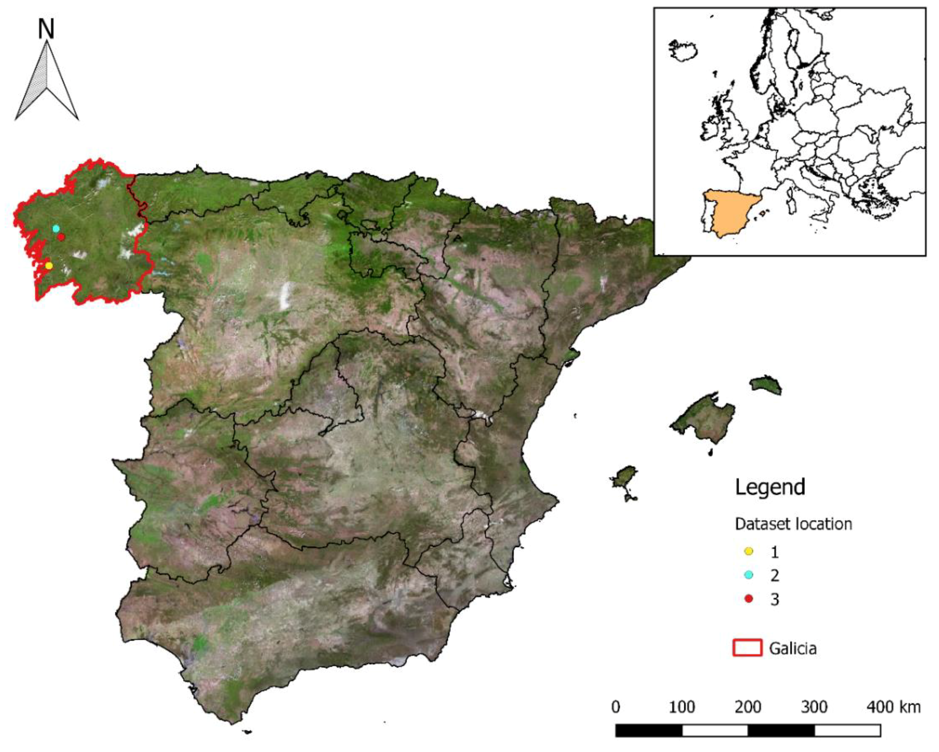
The methodology was tested in three LiDAR datasets, corresponding to different locations in Galicia, a region in the northwest of Spain (Figure 1).

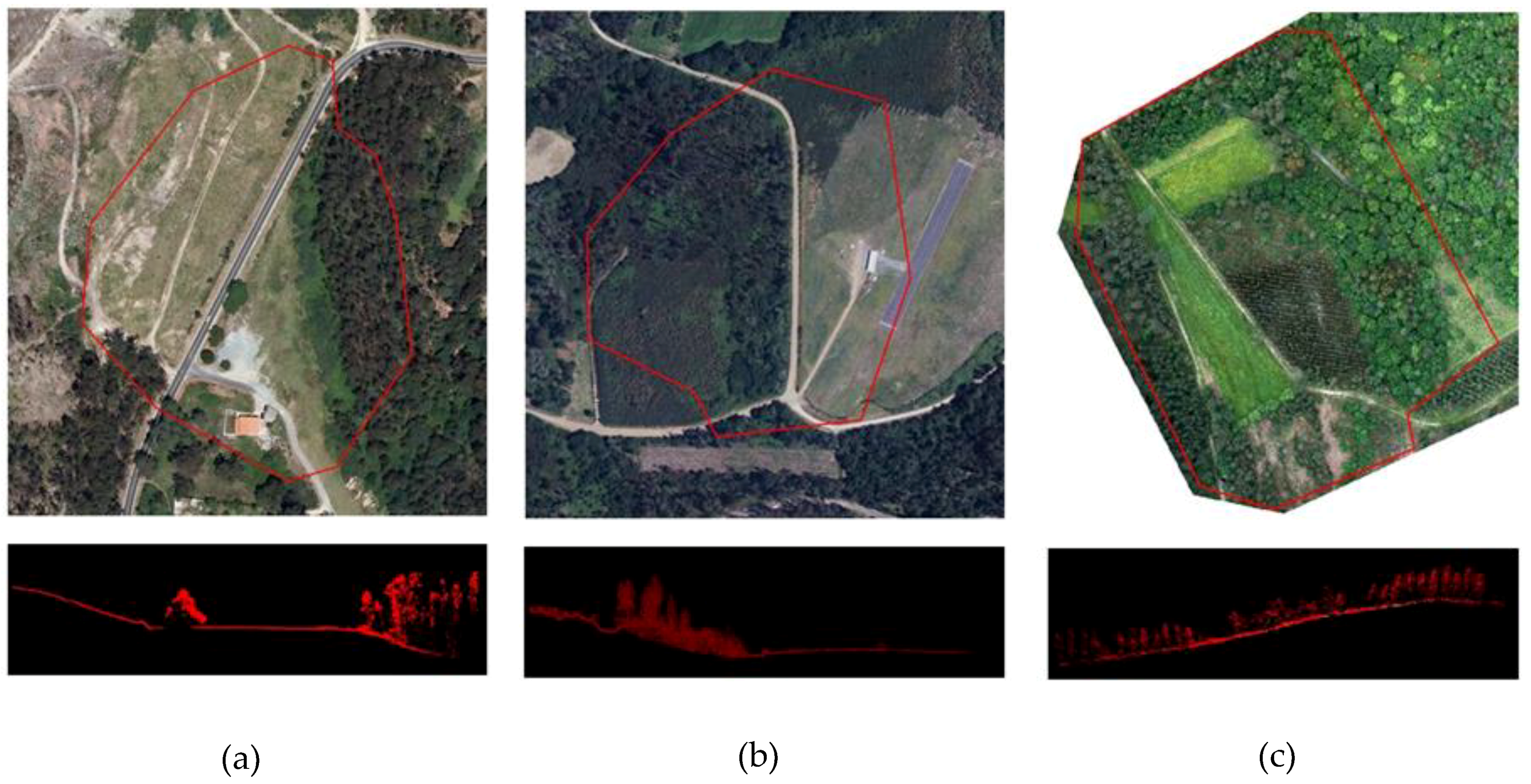
For this study, we selected three areas located next to buildings or roads. Dataset 1 is located in a WUI zone, which includes a pair of houses and a secondary road (Figure 2a). Eucalyptus globulus Labill. was the predominant species in this dataset. Additionally, there were other tree species in the dataset, such as Pinus pinaster Ait., Platanus x hispanica Mill. ex Muenchh, and Quercus sp. Almost all of the understory surface was dominated by herbaceous species.

Dataset 2 included roads and a sporting facility (Figure 2b). The mosaic of vegetation presented a high variability. A plantation of E. globulus existed in the southern part of the dataset, without a shrub understory. In the western part of the dataset, there were different overstory species, such as Quercus sp., E. globulus, and Pinus sp. The shrub load was high in this area and was formed by Ulex sp., Cystus sp., and Rubus sp. In addition, there was herbaceous vegetation close to the facilities.

Finally, Dataset 3 contained a young Eucalyptus nitens H. Deane & Maiden stand among other species, such as Pinus pinaster and other broadleaves (Figure 2c). The shrub load was high in some points of the set and was formed by Ulex sp., Cystus sp., and Rubus sp. There was a pasture near the road.

2.2. UAV LiDAR Datasets and Software Tools

The point clouds of three different forested sites were obtained using a Velodyne VLP 16 LiDAR unit (3.0.40.0, Velodyne LiDAR, San Jose, CA, USA). They were captured during leaf-on conditions in 2017 using a UAV platform. The covered surface, point cloud density, and point cloud size for each dataset are specified in

Table 1. Point cloud characteristics for each dataset.

Characteristic	Set 1	Set 2	Set 3
Number of Points	5,254,680	1,931,074	10,824,804
Point density (pts/m2)	107.9	21.83	124.06
Covered area (ha)	4.89	8.84	8.73

. Official thematic information, at a scale of 1:10,000 (dating from 2014), was used to obtain information about roads, power lines, buildings, etc.

The LiDAR data were processed with the free-license software, FUSION v.3.60 (USDA, Forest Service, PNRS, 2008), which was developed by the United States Department of Agriculture, US Forest Service, and Northwest Pacific Research Station (PNRS). GIS Quantum GIS (QGIS Development Team, 2009) was used to perform the geoprocessing and maps edition.

3. Methodology

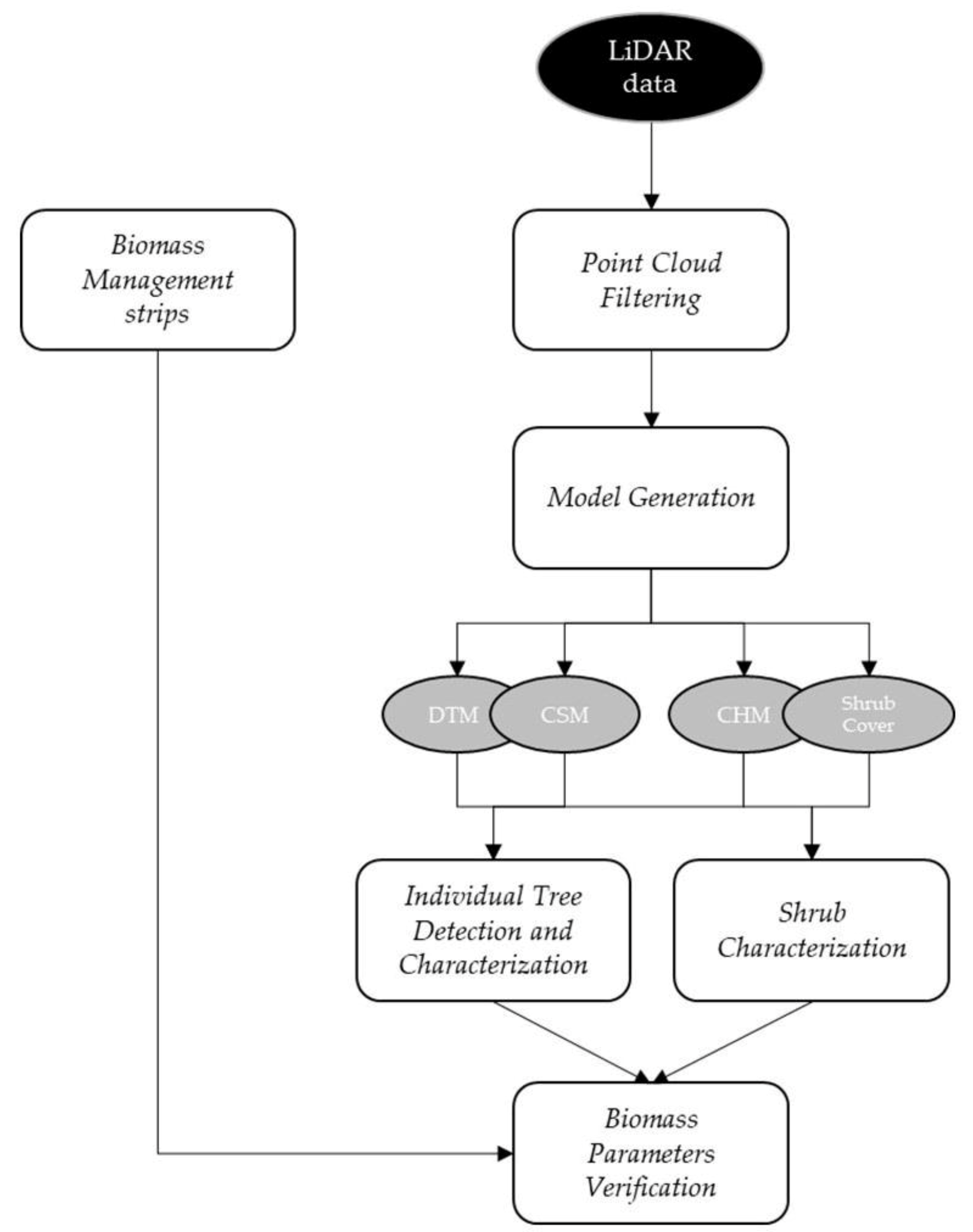
The proposed methodology is based on individual tree detection (ITD) and measurement over a LiDAR point cloud, acquired with a UAV platform (Figure 3). It starts with the detection of the biomass management strips (Appendix A), where the vegetation might be measured and controlled. Then, LiDAR-based models, such as terrain and canopy models, are obtained for further identification of the individual trees. Trees are geometrically characterized through the automatic measurement of the total height, pruning height (Appendix A), and crown diameter. A decision tree was designed and applied to check the legal conditions, and, finally, maps were generated to show the results.

3.1. Biomass Management Strips

The biomass management strip dimensions might be defined in consideration of the specifications, established in the wildfire prevention legislation. For the study area, they are defined as boundary regions around anthropogenic features (

Table 2. Legal buffer distances for the different forest biomass management networks and features.

Features	Biomass Management Networks	Buffer (m)
Public communication infrastructures	Primary network	5
Industry areas, buildings, recreational areas	Secondary network	50
Urban roads	Tertiary network	5
Forest roads	Tertiary network	2

). All of the features to be considered can be derived from official cartographic sources. The strips can be built by applying the corresponding buffers to every feature layer, obtaining the biomass management networks as a result.

3.2. LiDAR Point Cloud Filtering

Point cloud filtering is the first step of data processing and model generation. Several studies have recently been published regarding ground filtering algorithms for terrain modeling. Meng et al. [29] and Silva et al. [30] concluded that weighted linear least squares, which is based on linear prediction, provided accurate results in forest environments. In our case, the filtering algorithm that was used was based on Kraus and Pfeifer linear prediction [31], which was adapted from the Kraus and Mikhaiz method [32]. This consists of computing a surface with equal weights for every LiDAR point. In this study, the surface was obtained using a median filter and a focal mean filter of 5 × 5. The resultant surface lay between the true ground and the canopy surface. Terrain points are supposed to be below the surface and the vegetation points above it. The normal distance and direction of the point to surface vector is used to compute weights for LiDAR points. Successive surfaces are generated through an iterative process. Once the iterations are concluded, the terrain points are selected.

3.3. LiDAR-Based Modeling

Tree and shrub covers are modelled separately. First, Digital terrain models (DTM), canopy surface models (CSM), and canopy height models (CHM) might be generated. The CHM is essential to model vegetation height, and it can be obtained as the difference of the CSM and DTM. For DTM generation, the filtered point clouds might be used, and individual cell elevations are calculated using the minimum elevation of all points within the cell. According to Rowell et al. [33], a filter might be applied to the CHM in order to improve the predictions of tree detection algorithms. In this case, a median filter and a focal mean filter is used. A shrub cover digital surface can be computed as a function of the number of the LiDAR returns. Shrub heights are considered to range from 0.2 m (below this value, returns are supposed to be on the ground) to 3 m (above this value, returns are considered to be woodland). The value for every cell was obtained through Equation (1):

$$Shrub cover (\%)=\frac{number of all returns between 0.2 and 3 meters}{number of total returns in 5 meters cell}\times 100$$

(1)

3.4. Individual Tree Detection and Characterization

Tree characterization requires the prior identification of individuals. The individual tree detection process (ITD) or tree segmentation is considered crucial for wildfire prevention purposes, since it determines the confidence of the estimated maintenance actions and, consequently, the efficiency of the designed management. Vauhkonen et al. [34] reported that individual tree detection rates could range between 40% and 80% for different forest types, and Kaartinen et al. [35] reported a range between 40% and 90% for boreal conifers. According to Vaukonen et al. [34], the ITD is dependent on tree density and clustering, but not on the algorithm used. However, Ayrey et al. [36] pointed out that algorithm results were significantly dependent on the type of forest. Yu et al. [37] concluded that the tree density parameters did not significantly affect tree attribute estimation. Several ITD methods are available: variable-sized window (VSW), watershed delineation (WD), point cloud segmentation, layer stacking, etc. The VSW and WD methods are raster-based algorithms; they specifically use CHM. Point cloud segmentation and the layer stacking methods directly use the point cloud. The variable-sized window algorithm was developed by Popescu et al. [38]. This method uses a variable-sized window to identify the local maxima in a surface mesh. Watershed delineation creates a mesh through CHM inversion in order to detect the local minima of ridges and delineate adjacent individual tree crowns [16,26,39]. The point cloud segmentation method was developed by Li et al. [40]. First, the local maxima points are established, and points are iteratively assigned to trees based on a distance threshold. The layer stacking method was recently introduced by Ayrey et al. [36] and consists of slicing the point cloud and isolating the trees in each layer. The results are merged to produce tree profiles.

Some factors determine the final accuracy of the segmentation algorithms. They can be divided into two categories: stand characteristics and tree characteristics. The characteristics of the stand refer to the forest types (conifers/broadleaves/mixed), the tree density and spatial distribution, and the vertical structure. Tree characteristics refer to crown morphology and overlapping [34].

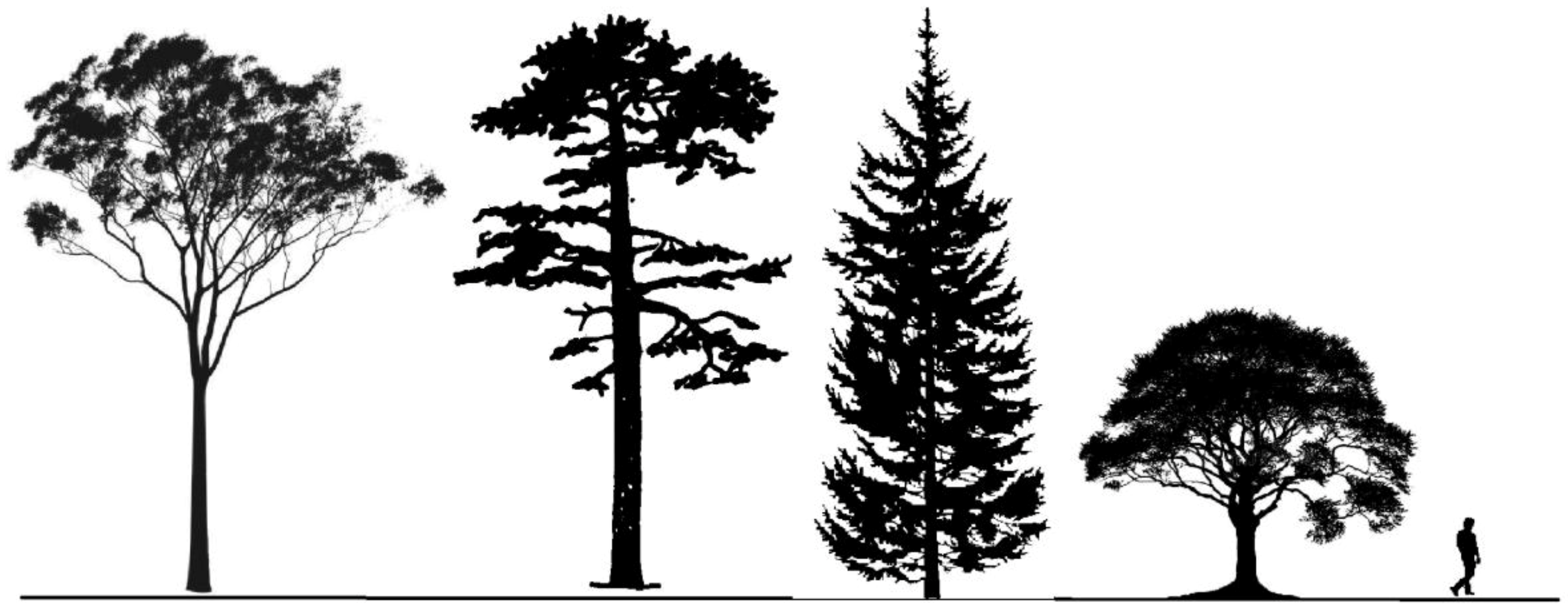
Significant differences in accuracy between forest types were reported by Vauhkonen et al. [34], where segmentation algorithms showed differences in the detection rates of between 40% and 80%. In general, tree identification algorithms obtain better results in coniferous stands than broadleaves. Differences between conifers and broadleaves range between 9% and 30% less [17,18], and, even in boreal conifers, Kaartinen et al. [35] reported a range between 40% and 90%. These differences can be explained by the crown morphology. The crown of coniferous trees tends to be conical, so defining the local maxima is easier than with non-conical shapes (Figure 4). Furthermore, broadleaves can present branches that might be interpreted as crowns for the algorithm and therefore may detect multiple trees in the same crown.

Important difficulties arise when these methods are applied to the point clouds of mix stands, especially for the VSW method. The ratio of crown width/total height (Appendix A) differs among species, so the window size is estimated with different coefficients. If the window size is adapted to the dominant species in the point cloud, the other species will be overestimated. Crown overlapping also involves some problems. Poor results are also obtained when the crowns overlap, which is especially frequent in deciduous stands [19] as well as stands with a complex vertical structure or stratification. In this case, both the raster-based and point cloud-based segmentation methods were unable to detect overtopped trees [20].

For the study cases, the raster-based algorithms were selected to be analyzed in detail, specifically the watershed delineation and variable-sized window methods.

3.4.1. Variable-Sized Window Method

This method uses Equation (2) to estimate the varying window size. The corresponding CHM was used as input data:

$$window size=A+B\times H_t+C\times H_t^2+D\times H_t^3+E\times H_t^4+F\times H_t^5$$

(2)

A, B, C, D, E, and F are constant coefficients, and H_t is the model height at the center of the window (in meters). As a result of the process, a vector file is obtained, which contains the georeferenced points, representing every individual tree in the analyzed forest stand.

3.4.2. Watershed Delineation

This method is based on image processing. As a result of the CHM inversion, the local maxima become the local minima and vice versa. In the image, trees appear as catchment basins, and region edges correspond to watershed lines. The aim of the algorithm is to find the watershed lines to isolate each region [17]. Some parameters can be configured, such as the maximum tree height, minimum tree height, buffer size, and Gaussian smooth options, as the sigma and radius.

3.4.3. ITD Verification

Field measurements were taken in the three analyzed sites. Samples of trees were georeferenced through GPS and characterized using inventory instruments (Vertex IV, Haglöf, Långsele, Sweden). Specifically, the total height and pruning height were measured. The GPS coordinates were used to define circumferences with a 2-m radius. Those points resulting from the ITD process within these circumferences were considered as correct identifications. The global accuracy and tree ratio were estimated. The global accuracy is obtained as the ratio of correct points in relation to the size of the sample. The tree ratio reflects the correspondence between the real number of trees in the stand and the estimated number.

3.4.4. Tree Characterization

The total height (H_t) and pruning height (H_pruning) were estimated for every identified tree. The total height values are directly obtained from the CHM cells that correspond to every identified tree. In relation to the pruning height values, FUSION estimates this parameter as 1/2 of H_t. However, this simplification is not assumable for the verification of legal geometric restrictions in wildfire prevention, since the authorized threshold for this parameter is 1/3 of the total tree height. According to the FUSION model, every analyzed tree will satisfy the pruning condition. Consequently, a descriptive model should be obtained. Different regression models were analyzed to estimate H_pruning as a function of H_t. Second-order polynomial models were selected for the analyzed datasets (Equation (3)). The field measurements were used for the model adjustments. A combined model was also evaluated. The model with the highest correlation coefficient was selected to estimate the pruning height of every detected individual tree as a function of the LiDAR height:

$$H_{pruning}=-C+B\times H_t-A\times H_t^2$$

(3)

3.5. Shrub Characterization

The wildfire prevention policy in the study area requires the verification of shrub geometric parameters. To this end, the shrub cover model obtained in Section 4.3 can be segmented in coverage intervals, according to the values that are described in the specific regulations.

3.6. Biomass Parameters Verification for Wildfire Prevention

Once individual trees have been characterized and shrubs have been modelled, geometric parameters can be compared with the restrictions that are specified in the wildfire prevention legislation. The specific parameters for the legislation in the study area are included in

Table 3. Geometric requirements for biomass management strips, established by the Galician wildfire prevention law [41].

Strata	Distance between Trees	Geometric Conditions
Overstory	≥7 m	Height ≤ 11.4 m	Pruning height < 35% of total height
		Height ≥ 11.4 m	Pruning height ≥ 4 m above ground
Understory	-	Cover < 20%	Height < 100 cm
		Cover 20%–50%	Height < 40 cm
		Cover > 50%	Height < 20 cm

. The comparison can be automated using logical functions.

4. Results

4.1. Biomass Management Strips

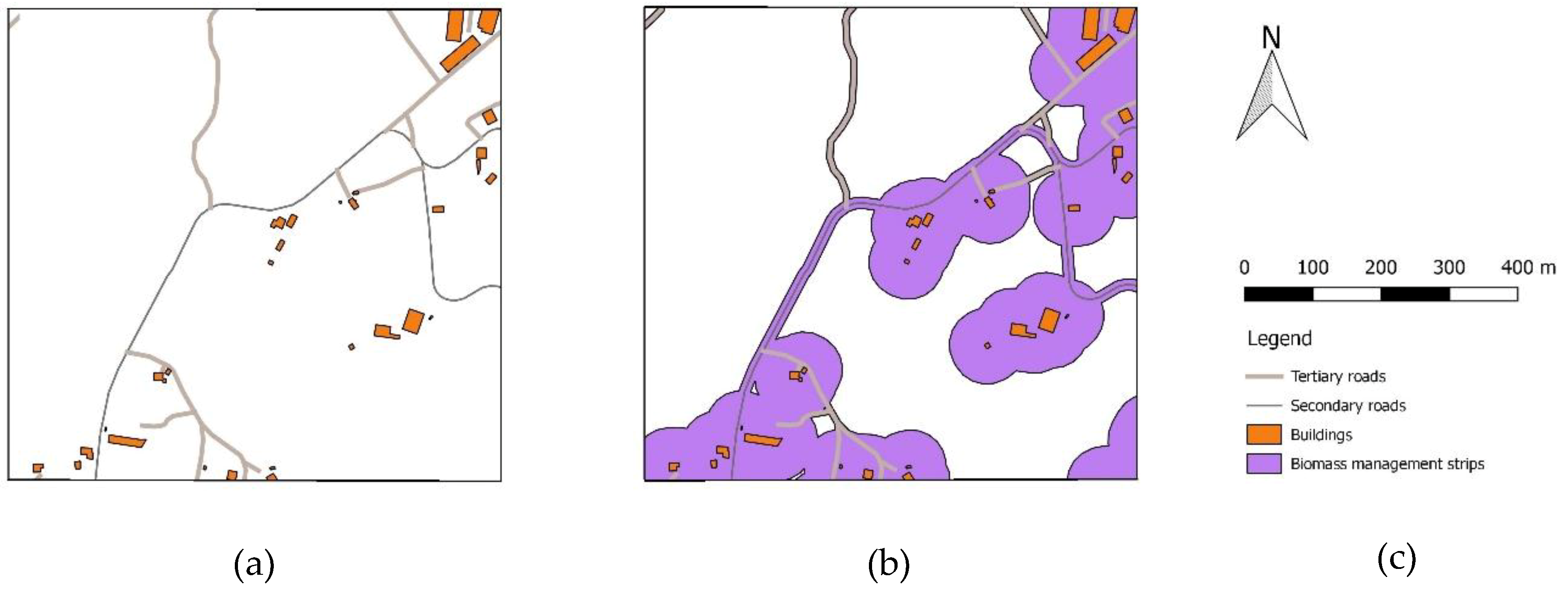
The biomass management strips for the study areas were defined in consideration of the specifications that are established in the regional wildfire prevention legislation (Table 2). The official cartographic series 1:10,000 provided the vector layers of all of the affected features to be considered. They were grouped to generate the corresponding networks (primary, secondary, tertiary) (Figure 5a). The appropriate buffers were applied to every network in order to obtain the biomass management strips, where vegetation might be totally or partially removed (Figure 5b).

4.2. LiDAR Point Cloud Filtering and Modelling

The LiDAR datasets contain information about forest cover, communication infrastructure, and some buildings. Buildings might be removed from the point clouds, since they can introduce errors in tree detection and shrub interpretation. To this end, the cartographic series at a low scale can be used. Specifically, the official cartographic series at a 1:10,000 scale was used. A 2-m buffer was applied to the buildings layer in order to solve the mismatching of contours in the point cloud. This final layer was used to subtract the building footprints from the LiDAR point clouds.

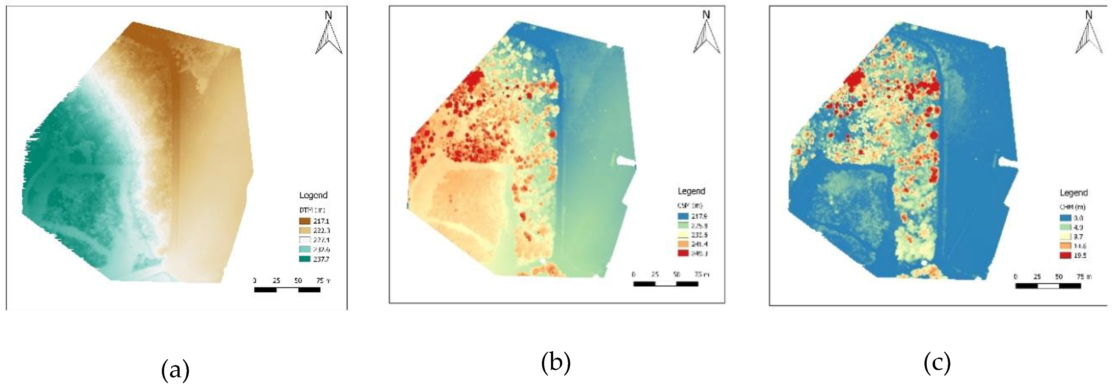
LiDAR point clouds were filtered to remove noise using the Kraus and Pfeifer linear prediction [31] method, which was explained in Section 3. Digital terrain models (DTM), canopy surface models (CSM), and canopy height models (CHM) were generated for the analyzed datasets. For DTM generation, the filtered point clouds were used. Cell sizes of 1.5 m were considered in order to avoid interpretation errors and empty holes. The resultant DTM model for Dataset 2 is shown in Figure 6a. The CSM was obtained using cell sizes of 0.25 m. The CHM was calculated as the difference of the CSM and DTM, obtaining a final model, with a 0.25-m spatial resolution. In the three cases, the CHM surfaces were smoothed by a 1.5 × 1.5 median window and a 2 × 2 smooth window. The resultant models for Dataset 2 are shown in Figure 6.

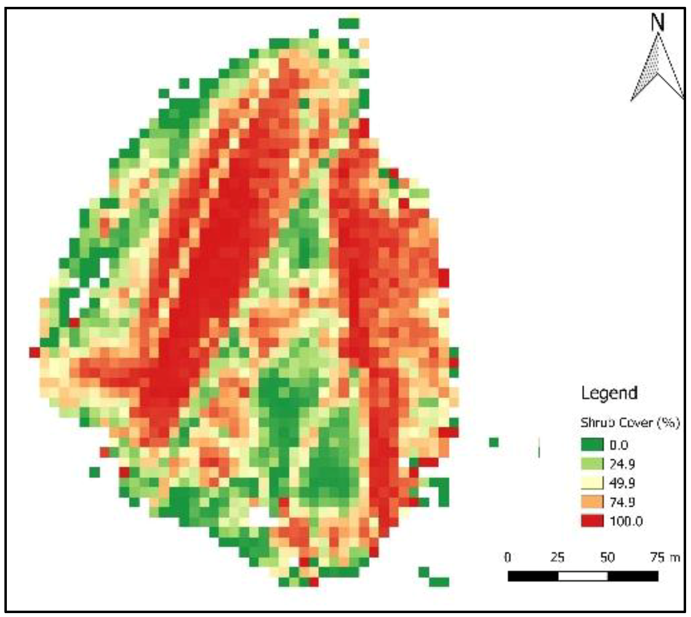
The shrub cover digital surface was obtained for the analyzed point clouds, with a 5-m resolution. The output values were expressed as percentages and represented using a false color palette (Figure 7).

4.3. Individual Tree Detection and Characterization

Set 1 and Set 2 were mixes of broadleaves, whose origin was predominantly natural regeneration, including seedlings as well as coppiced trees. Set 3 was composed of a young stand of broadleaves, wherein same-aged trees had a regular spatial distribution pattern. In this case, the crowns were well-defined and not overlapping. For these study cases, the raster-based algorithms were analyzed in detail, specifically the watershed delineation and variable-sized window methods, which were described in Section 3.

4.3.1. Variable-Sized Window Method

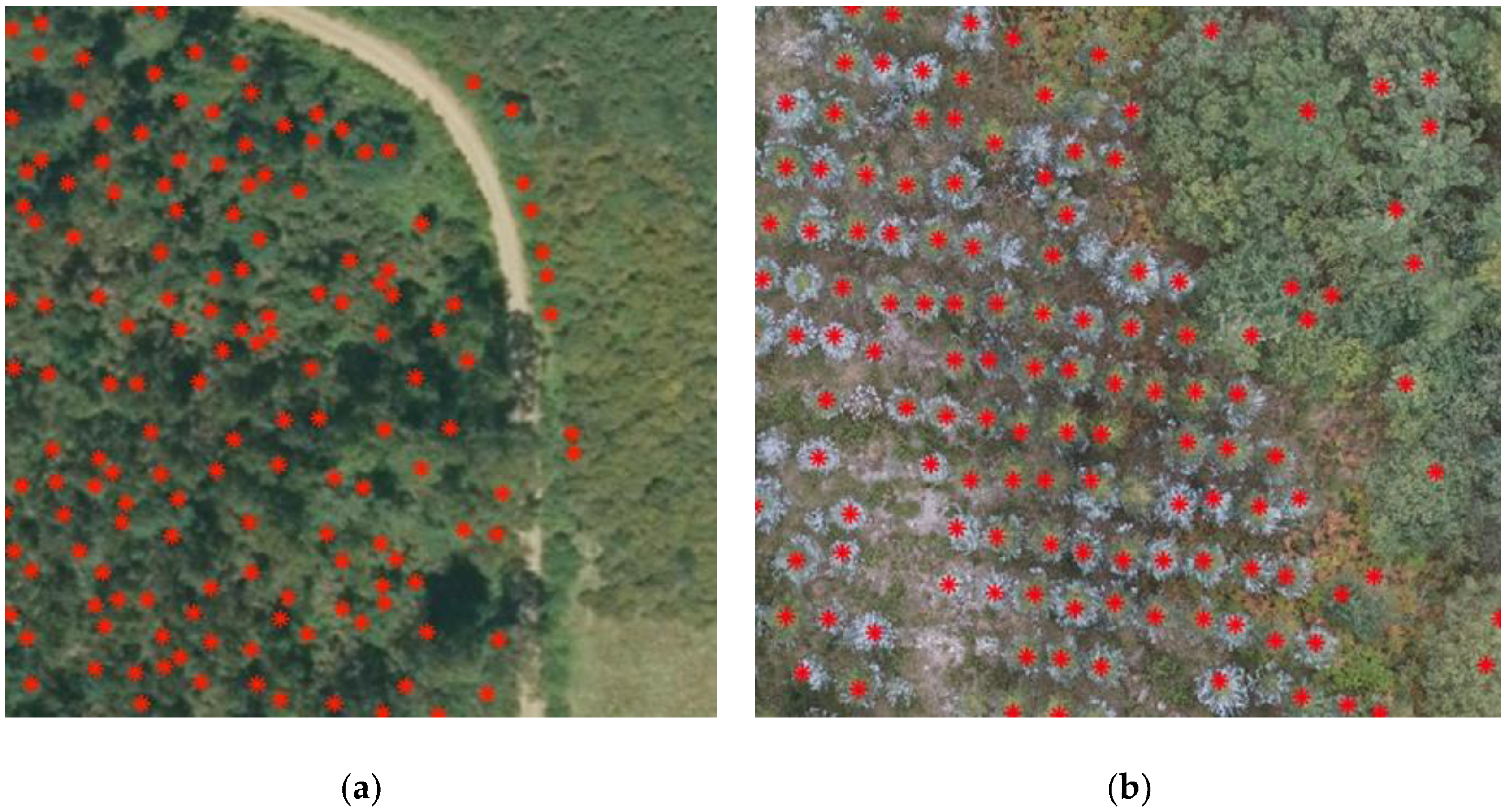
Since the algorithm has a better performance in relation to conifer trees than deciduous [42], the window size could be adapted to the species in the datasets of the study cases. The dominant species in the three sites was Eucalyptus sp. The equations of the window size were calculated by regression models, considering the total height (H_t) and crown width (C_w), as the independent variables. These were both estimated through the CHM. Different CHM resolutions and regression model functions were tested. The best prediction was obtained for Dataset 2 using a quadratic model. The parameters for the three regression models are specified in

Table 4. Estimation of the variable-sized window for ITD.

Dataset	CHM Resolution (m)	Constant Coefficients						R2
		A	B	C	D	E	F
1	0.25	0.9540	1.1533	−0.0014	0	0	0	0.25
2	0.25	3.1972	−0.0328	0.0059	0	0	0	0.55
3	0.5	2.5676	−0.1467	0.017	0	0	0	0.34

ITD: Individual Tree Detection; CHM: Canopy Height Model; A, B, C, D, E, F: constant coefficients.

. Figure 8 illustrates the identified individuals. In the managed forest (Dataset 3), the VSW provided satisfactory results.

4.3.2. Watershed Delineation

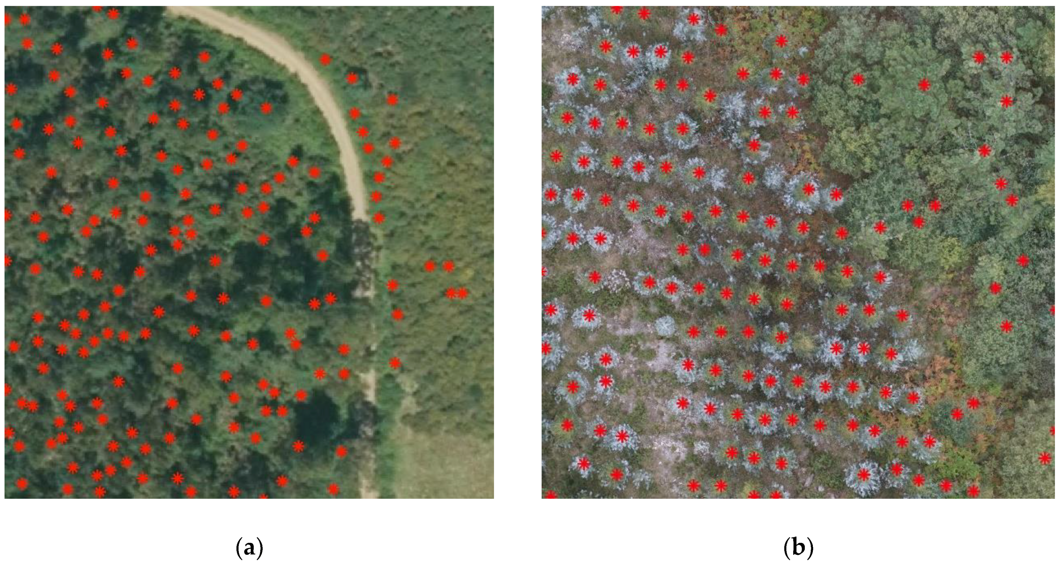
To implement this algorithm, the maximum and minimum heights were estimated, according to the values in the analyzed stands. Trees under 4 m were not considered in any case. The buffer size was indicated in pixels. Sigma is the value of the Gaussian smoothing factor; the greater the value, the higher the smoothness. Finally, the window size of the smooth filter was defined by the radius, and it is recommended to establish it as the average crown diameter size in pixels. The results of the segmentation process depend mainly on the sigma and the CHM spatial resolution. The parameters for each dataset are specified in

Table 5. Optimum configuration selected for each dataset for the watershed delineation algorithm.

Dataset	CHM Resolution (m)	Hmax	Hmin	Buffer	Gaussian Smooth
					Sigma	Radius
1	0.5	80	4	50	1.5	5
2	0.5	80	3	50	1.5	5
3	0.5	80	3	20	1	5

CHM: Canopy Height Model.

. Figure 9 illustrates the identified individuals. In the managed forest (Dataset 3), the WD provided satisfactory results.

4.3.3. ITD Verification

The reliability of the individual tree detection process, and the accuracy in their geopositioning, is evaluated through a sample of 137 trees, which were georeferenced through GPS and characterized using inventory instruments (Vertex IV), as described in Section 3. The best results correspond to the planted forest (Dataset 3): 85% for VWS, and 83% for WD. In this case, the number of trees was underestimated by both algorithms. For Datasets 2 and 3, which corresponded to the naturally regenerated forests, the VWS provided better results than the WD, and the tree ratio revealed that both algorithms overestimated the number of trees in this kind of stand (

Table 6. Verification results of the ITD algorithms for the three datasets.

	ITD Algorithm
	VWS		WD
	Accuracy	Tree Ratio	Accuracy	Tree Ratio
Set 1	0.58	1:1.29	0.52	1:1.37
Set 2	0.49	1:1.09	0.52	1:1.10
Set 3	0.85	1:0.85	0.83	1:0.89
Average	0.64		0.62

ITD: Individual Tree Detection; VSW: Variable-Sized Window; WD: Watershed Delineation.

).

4.3.4. Tree Characterization

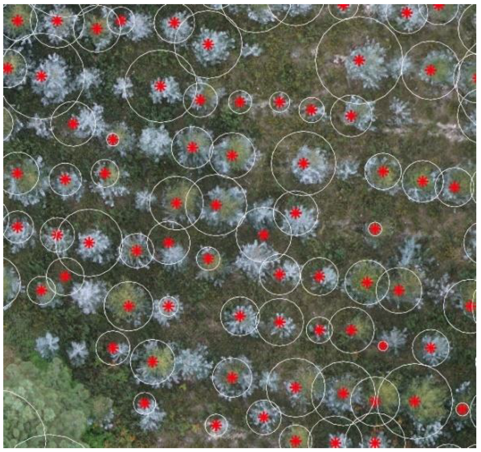
The VSW algorithm was used to identify the individual trees and obtain their characteristics in the study cases. All points that were identified in the boundary of the LiDAR point cloud were excluded from the analysis to minimize errors. The final sample numbers were 230 trees for study case 1; 1063 trees for study case 2; and 2507 trees for study case 3 (Figure 10).

The total height (H_t) values were obtained for every detected individual tree from the corresponding CHM cell. For the pruning heights, second-order regression models were evaluated. The best correlation coefficient was obtained for the combined model (see

Table 7. Estimation of pruning height using different regression models.

Dataset	A	B	C	R2
1	−0.0093	0.7505	−1.8945	0.48
2	−0.003	0.6151	−1.6364	0.70
3	−0.0154	0.5335	−0.6039	0.33
1–2–3	−0.0032	0.5822	−1.4195	0.72

). This model was used to estimate the pruning height of every individual tree.

The resulting pruning heights as well as the total heights were compared with the field measurements. Resulting mean errors, standard deviations, and Root-mean-square errors (RMSE) are shown in

Table 8. Accuracy assessment of total height regression models for every dataset: Mean errors and Root-mean-square errors (RMSE).

Dataset	Total Height
	Mean Error	RMSE
1	−0.78	1.82
2	0.11	2.51
3	0.22	0.94

and

Table 9. Accuracy assessment of pruning height regression model for every dataset: Mean errors, standard deviations and Root-mean-square errors (RMSE).

	Pruning Height—Combined Regression Model
Dataset	Mean Error	Standard Deviation	RMSE
1	−0.92	3.12	3.14
2	0.33	2.70	2.69
3	1.02	1.08	1.48

.

4.4. Shrub Characterization

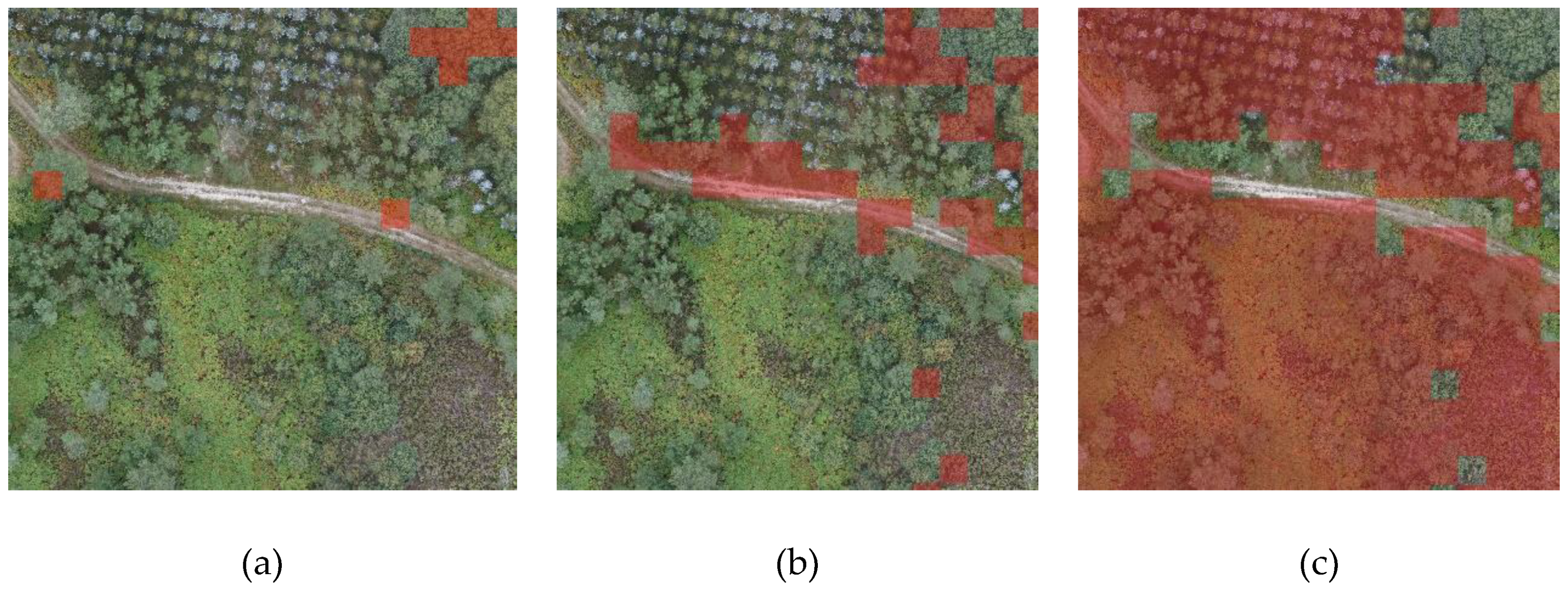
The shrub cover model obtained for every dataset was segmented in three coverage intervals, according to the values specified in the regional fire prevention law: >50%, 20%–50%, and <20% (Figure 11).

4.5. Biomass Parameters Verification for Wildfire Prevention

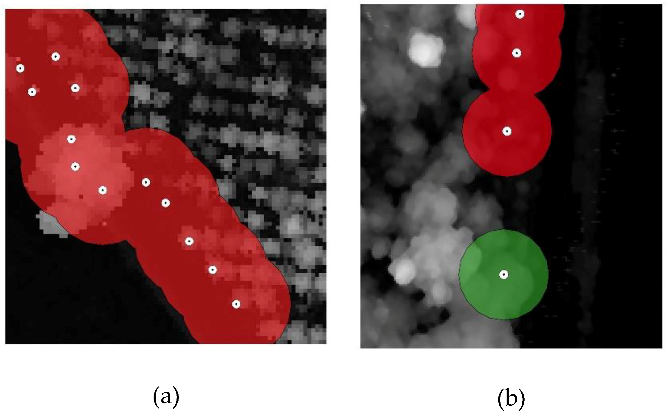
For the study sites, the biomass management strips included 54 trees and 10,563 m² of shrub in Dataset 1, 19 trees and 10,783 m² of shrub in Dataset 2, and 94 trees and 6041 m² in Dataset 3. The characteristic geometric descriptors of every single tree were compared with the legal specifications using logical functions and compiled in a decision tree (Figure 12). The results of the tree verification are described in

Table 10. Results of the vegetation verification in the biomass management strips for each dataset. Pruning height and density criteria were verified for trees and cover, and height criteria were verified for shrubs.

	Tree Verification (Number of Trees)			Shrub Verification (m2)
	Pruning Height		Density	Cover and Height
	Does Not Comply	Comply	Does Not Comply	Allowed	Not Allowed
Dataset 1	10	44	52	5.658 m2	4.905 m2
Dataset 2	4	15	16	7.590 m2	3.193 m2
Dataset 3	22	72	90	2.056 m2	3.985 m2

. The condition of spacing among individuals, which is equivalent to 510 trees/hectare, was checked though Quantum GIS tools. A 7-m buffer was applied to every single tree, and those that presented an overlap were dissolved. The surface of these new polygons was analyzed. The area of each polygon should be 153.97 m², and all those with a higher value corresponded to pairs or groups of trees that did not satisfy the spacing condition (Figure 13).

In the case of shrubs, the allowed spacing is expressed as ranges of ground cover, as shown in Table 3. For every cover range, a maximum vegetation height is allowed. In this case, the shrub cover model and CHM were used for the verification of these legal conditions. Conditional functions were applied and were compiled in a decision tree (Figure 14). A color code was used to show the allowed and not allowed conditions.

The overall results of the legal verification process are shown in Table 10. In Dataset 1, a total of 54 trees was located in the biomass management strips, where 19% of the trees did not comply with the current legislation requirement in terms of pruning height, 96% of the trees did not comply in terms of density criteria, and 46% of the surface of shrubs might be managed. In Dataset 2, a total of 19 trees were located in the biomass management strips, where 21% of the trees did not comply with the current legislation in terms of pruning height, 84% of the trees did not comply in terms of density criteria, and 30% of the surface of shrubs might be managed. In Dataset 3, a total of 94 trees were located in the biomass management strips, where 23% of the trees did not comply with the current legislation in terms of pruning height, 96% of the trees did not comply in terms of density criteria, and 66% of the surface of shrubs might be managed.

4.6. Legal Compliance Validation

In order to verify the reliability of the described process in the legal verification of the geometric restrictions in the biomass management strips, a confusion matrix was generated, together with the corresponding global accuracy. The different models to estimate H_pruning were evaluated. The results are shown in

Table 11. Accuracy assessment of the legal requirement verification. The different H_pruning models are evaluated.

Dataset	Biomass Management Strips Verification
1	0.88
2	0.72
3	0.51

.

5. Discussion of Results

The legal verification of geometric parameters and spacing conditions in biomass management strips requires individual tree detection, total height estimation, pruning height estimation, and spacing evaluation. For shrubs, H_t and cover are required. High-density LiDAR point clouds were used to model the terrain and characterize the forest canopy. Three different study areas were used, and two of them corresponded to naturally regenerated stands, with different species, crown morphologies and tree ages. One of the study sites corresponded to a plantation, with one dominant species, and a homogeneous age, but varying crown sizes.

For the identification of individual trees, two raster-based tree segmentation algorithms were analyzed in detail: VWS and WD. In the VWS algorithm, the window size was associated with crown width and was estimated as a function of H_t and several constant coefficients. The equation to estimate the window size was obtained through regression models. For every analyzed case study, crown width and H_t did not show a strong relationship. Dataset 2 had the best performance, with an R² = 0.54, and Dataset 1 had the worst, with an R² = 0.25 (Table 6). Even in Dataset 3, corresponding to the regular stand, in terms of age and spacing, the correlation was poor (R² = 0.34). However, previous studies have reported similar results. Morsdorf et al. [22] obtained a coefficient of determination between 0.20 and 0.43 for boreal species.

The difference between the VWS and WD algorithms was not significant. The overall accuracy of VWS was 2% higher than the WD overall accuracy, and the tree ratio in the VWS algorithm was slightly closer to a 1:1 ratio than that in the WD algorithm (Table 6). For both algorithms, the number of trees was overestimated in the datasets of natural regeneration (Datasets 1 and 2), while it was underestimated in the plantation (Dataset 3).

The accuracy of tree detection was very high for the plantation sample for both algorithms: 85% in the VWS (Table 6), while in the naturally regenerated samples, the results were poor (58% and 49% in the VWS). These results reveal the influence of the homogeneous species composition, regular distribution pattern of the individuals, and the conical shape of the crowns, which characterize the young planted stand (Dataset 3). However, the lower accuracy in the other datasets might be due to the non-conical shaped crowns; branches can provide multiple detections, which result in false positives; and in coppices, this effect might be stronger. The high tree ratio in Dataset 2 might also be explained by the presence of some old bushes that reached 4 m high; these could also provide false positives. Furthermore, this dataset presented the highest structural complexity. In any case, these results were consistent with other studies that demonstrated global accuracies ranging from 32% to 66% using the VWS algorithm [25,36].

The LiDAR-based estimations of the total height of individuals were slightly overestimated in Datasets 2 and 3 (Table 8). However, the LiDAR height estimations were slightly higher than the Vertex measurements in Dataset 1. Several factors might be considered to explain these discrepancies. The date of LiDAR acquisition and field work could introduce significant deviations in Dataset 2; they differed by one and a half years in this study case. Eucalyptus stands at young ages in the best sites could reach annual growths of 2 m per year in Galicia. The error associated with the Vertex estimations was also relevant. In round shaped crowns, the H_t is frequently overestimated when the tree top is pointed. Furthermore, Vertex measurements are affected by operation errors, such as stand passability, tree density, canopy closure, and operator skills, which affect the accuracy of the measurements. These errors, as well as the way they affect the derived models, have rarely been reported or estimated [43,44]. Nevertheless, previous works have reported similar LiDAR-Vertex discrepancies in height estimations [45], with values between 0.8 and 1.3 m in deciduous and coniferous plots [34], and R² between 0.54 and 0.71 [46], R² = 0.79 [25], or even R² = 0.92 [22] in coniferous stands.

Similar results were obtained for pruning heights, with mean errors below 1 m (Table 9). These models were also affected by the explained limitations of the instruments that were used in the field work. Other authors, such as Gonzalez-Obarria et al. [23], also obtained similar results in conifer stands (R² = 0.54). According to the literature, the vegetation structure could be better characterized using a full waveform LiDAR due to its ability to digitize and record the entire backscattered signal of each laser pulse [47,48]. Andersen et al. [12], achieved an R² = 0.77 in CBH estimation using a small footprint full-waveform LiDAR.

The verification of legal geometric requirements for the individual trees in the biomass management strips showed that the correct prediction was over 70% for two samples (Table 11); for the third, it was over 50%. These results could be explained by the age of the individuals and morphology. Generally, pruning heights are proportional to total heights. Young trees tend to have first brunches at lower levels than mature individuals. Consequently, the relative errors for pruning height estimations have a higher impact in the verification processes. This was the case with Dataset 3 of the analyzed case studies. As a result, it can be concluded that mature stands can be efficiently analyzed using the described methodology.

6. Conclusions

The extreme behavior of the wildfires that have occurred in recent years in Spain has pushed authorities to focus efforts on wildfire prevention. This paper presented a methodology using high-resolution LiDAR point clouds in forest vegetation characterization to improve the protection capabilities of the WUI and infrastructures. A UAV platform was used to acquire data in three different case studies, with varying species composition, density, homogeneity, and age. To verify the wildfire prevention legal restrictions, the vegetation included in the biomass management strips was analyzed. Individual trees were detected and characterized: parameters of height, pruning height, and spacing were obtained. The cover and height for shrubs were also estimated. The results were compared with field measurements, obtained using traditional instruments. Decision trees were built to automatically verify the geometric parameters.

The proposed methodology allows for the automatic verification of the compliance of vegetation in relation to the geometric restrictions established in wildfire prevention legislation. The subjectivity or skill of the operators is avoided, and the efficiency in the evaluation of large areas is significantly higher than in conventional methods. While a UAV based solution, like the described one, cannot be applied at the regional level, it can be successfully applied at a low scale for the evaluation of wildland urban interfaces, sensible areas around settlements or heritage sites, or areas with an extremely high wildfire frequency. The application of this methodology would allow for the detection of areas with a high level of non-compliance. This information might be essential to design intervention priority criteria in relation to wildfire prevention actions. Furthermore, it can easily be connected with administrative punitive procedures. Finally, the cartography of biomass strips, with their geometric characteristics, can be very helpful for wildfire suppression services in the planning of specific interventions.

References

1. Rowell, A.; Moore, P. Global Review of Forest Fires; WWF, IUCN: Gland, Switzerland, 2000. [Google Scholar]
2. Comisión Europea. Comunicación de la Comisión al Parlamento Europeo, al Consejo y al Comité de las Regiones: Reforzar la gestión de catástrofes de la UE: rescEU Solidaridad con Responsabilidad; Comisión Europea: Bruselas, Belgium, 2017. [Google Scholar]
3. Joint Research Center. Forest Fires in Europe 2004. European Communities: Italy, 2005; Available online: http://effis.jrc.ec.europa.eu/media/cms_page_media/40/04-forest-fires-in-europe-2004.pdf (accessed on 10 February 2019).
4. Martín, L.G. Spatial planning experiences for vulnerability reduction in the wildland-urban interface in Mediterranean European countries. Eur. Countrys. 2017, 9, 577–593. [Google Scholar] [CrossRef]
5. MAPAMA. Los Incendios Forestales en España; Ministerio de Agricultura y Pesca, Alimentación y Medio Ambiente: Madrird, Spain, 2017.
6. Aguilera, F.; Botelquilha-Leitao, A. Selección de métricas de paisaje mediante análisis de componentes principales para la descripción de los cambios de uso y cobertura del suelo del Algarve, Portugal. GeoFocus Rev. Int. Cienc. Tecnol. 2012, 12, 93–121. [Google Scholar]
7. Gallardo, M.; Martínez-Vega, J. Three decades of land use changes in region of Madrid and how they relate to territorial planning. Eur. Plan. Stud. 2016, 5, 1016–1033. [Google Scholar] [CrossRef]
8. Forest Service, USDA and USDI. Urban wildland interface communities within the vicinity of federal lands that are at high risk from wildfire. Fed. Regist. 2001, 66, 751–777. [Google Scholar]
9. Martínez, J.; Vega-García, C.; Chivieco, E. Human-caused wildfire risk rating for prevention planning in Spain. J. Environ. Manag. 2009, 90, 1241–1252. [Google Scholar] [CrossRef] [PubMed]
10. Rothermel, R.C. How to Predict the Spread and Intenisty of Forest and Range Fires; USDA: Ogden, UT, USA, 1983.
11. Comissao Técnica Independiente, Asamblea da República. Análise e apuramento dos factos relativos aos incendios que ocorreram em Pedrogao Grande, Castanheira de Pera, Ansiao, Alvaiázere, Figueiró dos Vinhos, Arganil, Góis, Penela, Pampilhosa da Serra, Oleiros e Serta, entre 17 e 24 de junho de 2017; Asamblea da República: Lisboa, Portugal, 2017. [Google Scholar]
12. Andersen, H.E.; McGaughey, R.J.; Reutebuch, E. Estimating forest canopy fuel parameters using LIDAR data. Remote Sens. Environ. 2005, 94, 441–449. [Google Scholar] [CrossRef]
13. Consellería del Medio Rural. ORDEN de 31 de Julio de 2007 por la que se Establecen los Criterios Para la Gestión de la Biomasa Vegetal. DOG, Agosto 7, 2007. Available online: https://www.xunta.gal/dog/Publicados/2007/20070807/Anuncio2E6AA_es.html (accessed on 2 April 2018).
14. Brandtberg, T. Classifying individual tree species under leaf-off and leaf-on conditions using airborne lidar. ISPRS J. Photogramm. Remote Sens. 2007, 6, 325–340. [Google Scholar] [CrossRef]
15. Chas Amil, M.L.; Touza, J.; García Martínez, E.D. Delimitación de la Interfaz Urbano-Forestal en Galicia: Análisis del riesgo de incendio. In Proceedings of the 6° Congreso Forestal Español, Vitoria-Gasteiz, Spain, 10–14 June 2013. [Google Scholar]
16. Kwak, D.A.; Lee, W.K.; Lee, J.H.; Biging, G.S.; Gong, P. Detection of individual trees and estimation of tree height using LiDAR data. J. For. Res. 2007, 12, 425–434. [Google Scholar] [CrossRef]
17. Ke, Y.; Quackenbush, L. Comparison of individual tree crown detection and delineation methods. In Proceedings of the 2008 ASPRS Annual Conference (American Society of Photogrammetry and Remote Sensing, Bethesda, Maryland), Portland, OR, USA, 28 April–2 May 2008. [Google Scholar]
18. Mei, C.; Durrieu, S. Tree crown delineation from digital elevation models and high resolution imagery. Proc. Int. Arch. Photogramm. Remote Sens. 2004, 36, 3–6. [Google Scholar]
19. Koch, B.; Heyder, U.; Weinacker, H. Detection of individual tree crowns in airborne Lidar data. Photogramm. Eng. Remote Sens. 2006, 7, 357–363. [Google Scholar] [CrossRef]
20. Koch, B.; Kattenborn, T.; Straub, C.; Vauhkonen, J. Segmentation of Forest to Tree Objects; Springer: Dordrecht, The Netherlands, 2014. [Google Scholar]
21. Alcasena, J.; Salis, M.; Vega-García, C. A fire modeling approach to assess wildfire exposure of valued resources in central Navarra, Spain. Eur. J. For. Res. 2016, 135, 87–107. [Google Scholar] [CrossRef]
22. Morsdorf, F.; Meier, E.; Kötz, B.; Itten, K.I.; Dobbertin, M.; Allgöwer, B. LIDAR-based geometric reconstruction of boreal type forest stands at single tree level for forest and wildland fire management. Remote Sens. Environ. 2004, 92, 353–362. [Google Scholar] [CrossRef]
23. González-Olabarria, J.-R.; Rodríguez, F.; Fernández-Landa, A.; Yudego, B.M. Mapping fire risk in the Model Forest of Urbión (Spain) based on airborne LiDAR measurements. For. Ecol. Manag. 2012, 282, 149–156. [Google Scholar] [CrossRef]
24. Ager, A.A.; McMahan, A.J.; Barrett, J.J.; McHugh, C.W. A simulation study of thinning and fuel treatments on a wildland–urban interface in eastern Oregon, USA. Landsc. Urban Plan. 2007, 80, 292–300. [Google Scholar] [CrossRef]
25. Hermosilla, T.; Ruiz, L.A.; Kazakova, A.N.; Coops, N.C.; Moskal, L.M. Estimation of forest structure and canopy fuel parameters from small-footprint full-waveform LiDAR data. Int. J. Wildland Fire 2014, 23, 224–233. [Google Scholar] [CrossRef] [Green Version]
26. Chen, Q.; Baldocchi, D.; Gong, P.; Kelly, M. Isolating individual trees in a savanna woodland using small footprint LiDAR data. Photogramm. Eng. Remote Sens. 2006, 72, 923–932. [Google Scholar] [CrossRef]
27. Mutlu, M.; Popescu, S.C.; Zhao, K. Sensitivity analysis of fire behavior modeling with LIDAR-derived surface fuel maps. For. Ecol. Manag. 2008, 256, 289–294. [Google Scholar] [CrossRef]
28. Riaño, D.; Chuvieco, E.; Ustin, S.L.; Salas, J.; Rodríguez-Pérez, J.R.; Ribeiro, L.M.; Viegas, D.X.; Moreno, J.M.; Fernández, H. Estimation of shrub height for fuel-type mapping combining airborne LiDAR and simultaneous color infrared ortho imaging. Int. J. Wildland Fire 2007, 16, 341–348. [Google Scholar] [CrossRef]
29. Meng, X.; Currit, N.; Zhao, K. Ground filtering algorithms for airborne LiDAR data: A review of critical issues. Remote Sens. 2010, 2, 833–860. [Google Scholar] [CrossRef]
30. Silva, C.A.; Klauberg, C.; Hentz, A.M.K.; Corte, A.P.D.; Ribeiro, U.; Liesenberg, V. Comparing the performance of ground filtering algorithms for terrain modeling in a forest environment using airborne LiDAR data. Floresta Ambiente 2018, 25, 1–10. [Google Scholar] [CrossRef]
31. Kraus, K.; Pfeifer, N. A new method for surface reconstruction from laser scanner data. Int. Arch. Photogramm. Remote Sens. 1997, 32, 80–86. [Google Scholar]
32. Kraus, K.; Mikhail, E.M. Linear least squares interpolation. Photogramm. Eng. Remote Sen. 1972, 38, 1016–1029. [Google Scholar]
33. Rowell, E.; Seielstad, C.; Vierling, L.; Queen, L.; Shepperd, W. Using laser altimetry-based segmentation to refine automated tree identification in managed forests of the Black Hills, South Dakota. Photogramm. Eng. Remote Sens. 2006, 72, 1379–1388. [Google Scholar] [CrossRef]
34. Vauhkonen, J.; Ene, L.; Gupta, S.; Heinzel, J.; Holmgren, J.; Pitkänen, J.; Solberg, S.; Wang, Y.; Weinacker, H.; Hauglin, M.; et al. Comparative testing of single-tree detection algorithms under different types of forest. Forestry 2012, 85, 24–40. [Google Scholar] [CrossRef]
35. Kaartinen, K.; Hyyppä, J.; Yu, X.; Vastaranta, M.; Hyyppä, H.; Kukko, A.; Holopainen, M.; Heipke, C.; Hirschmugl, M.; Morsdorf, F.; et al. An international comparison of individual tree detection and extraction using airborne laser scanning. Remote Sens. 2012, 4, 950–974. [Google Scholar] [CrossRef]
36. Ayrey, E.; Fraver, S.; Kershaw, J.A., Jr.; Kenefc, L.S.; Hayes, D.; Weiskittel, A.R.; Roth, B.E. Layer stacking: A novel algorithm for individual forest tree segmentation from LiDAR point clouds. Can. J. Remote Sens. 2017, 43, 16–27. [Google Scholar] [CrossRef]
37. Yu, X.; Hyyppä, J.; Vastaranta, M.; Holopainen, M.; Viitala, R. Predicting individual tree attributes from airbone laser point clouds based on the random forests technique. Isprs J. Photogramm. Remote Sens. 2011, 66, 28–37. [Google Scholar] [CrossRef]
38. Popescu, S.C.; Wynne, R.H.; Nelson, R.F. Estimating plot-level trees heights with LiDAR: Local filtering with a canopy height based variable window size. Comput. Electron. Agric. 2002, 37, 71–95. [Google Scholar] [CrossRef]
39. Soille, J. Segmentation. In Morphological Image Analysis: Principles and Applications; Springer: New York, NY, USA, 2009. [Google Scholar]
40. Li, W.; Guo, Q.; Jakubowski, M.K.; Kelly, M. A new method for segmenting individual trees from the lidar point cloud. Photogramm. Eng. Remote Sens. 2012, 78, 75–84. [Google Scholar] [CrossRef]
41. Xunta de Galicia. Ley 3/2007, de 9 de Abril, de Prevención y Defensa Contra los Incendios Forestales de Galicia. Available online: https://www.boe.es/buscar/act.php?id=BOE-A-2007-10022&p=20171228&tn=1#a20 (accessed on 4 April 2018).
42. USDA, Forest Service, PNRS. FUSION Software Manual, 2008. Available online: http://forsys.cfr.washington.edu/Software/FUSION/FUSION_manual.pdf (accessed on 7 June 2017).
43. Collins, B.M.; Stephens, S.L.; Roller, G.B.; Battles, J.J. Simulating fire and forest dynamics for a landscape fuel treatment project in the Sierra Nevada. For. Sci. 2011, 57, 77–88. [Google Scholar]
44. Jakubowski, M.K.; Guo, Q.; Collins, B.; Stephens, S.; Kelly, M. Predicting surface fuel models and fuel metrics using Lidar and CIR imagery in a dense, mountainous forest. Photogramm. Eng. Remote Sens. 2013, 79, 37–49. [Google Scholar] [CrossRef]
45. Hyyppae, J.; Kelle, O.; Lehikoinen, M.; Inkinen, M. A segmentation-based method to retrieve stem volume estimates from 3-d tree height models produced by laser scanners. IEEE Trans. Geosci. Remote Sens. 2001, 39, 969–975. [Google Scholar] [CrossRef]
46. Shiota, H.; Tanaka, K.; Nagashima, K. LiDAR data analysis with Fusion/LDV for individual tree measurement. J. Biodivers. Manag. For. 2017. [Google Scholar] [CrossRef]
47. Dubayah, R.O.; Drake, J.B. Lidar remote sensing for forestry. J. For. 2000, 98, 44–46. [Google Scholar]
48. Bye, I.J.; North, P.R.J.; Los, S.O.; Kljun, N.; Rosette, J.A.B.; Hopkinson, C.; Chasmer, L.; Mahoney, C. Estimating forest canopy parameters from satellite waveform LiDAR by inversion of the FLIGHT three-dimensional radiative transfer model. Remote Sens. Environ. 2017, 188, 177–189. [Google Scholar] [CrossRef]
Figure 1. Location of the three datasets in Galicia (red line), Spain.
Forests 10 00148 g001
Figure 2. Aerial photography and LiDAR profile of Dataset 1 (a), Dataset 2 (b), and Dataset 3 (c).
Forests 10 00148 g002
Figure 3. Process flow diagram of the applied methodology. DTM: Digital Terrain Model, CSM: Canopy Surface Model, CHM: Canopy Height Model.
Forests 10 00148 g003
Figure 4. Different species have different morphological characteristics of the crown. From left to right: eucalyptus silhouette; red pine silhouette; Douglas fir silhouette; and oak silhouette.
Forests 10 00148 g004
Figure 5. Process of creating the biomass management strips: (a) infrastructure layers in Dataset 1 (buildings, tertiary and secondary roads); (b) biomass management strips (purple polygons), created by means of infrastructure layers; and (c) legend and graphic scale.
Forests 10 00148 g005
Figure 6. Different models generated for Dataset 2: (a) Digital Terrain Model (DTM); (b) Canopy Surface Model (CSM); and (c) Canopy Height Model (CHM). Heights are expressed in meters.
Forests 10 00148 g006
Figure 7. Shrub cover model, generated by the LiDAR point cloud for Dataset 1.
Forests 10 00148 g007
Figure 8. Results of the Variable-Sized Window (VSW) process for Dataset 2 (a) and Dataset 3 (b). Trees are represented by red dots.
Forests 10 00148 g008
Figure 9. Results of the Watershed Delineation (WD) process for Dataset 2 (a) and Dataset 3 (b). Trees are represented by red dots.
Forests 10 00148 g009
Figure 10. Trees identified in Dataset 3, with the estimated crown diameters. Trees are represented by red dots.
Forests 10 00148 g010
Figure 11. Results of shrub characterization: red color represents the shrub with a cover of <20% in (a); the shrub with a cover between 20% and 50% (b); and the shrub with a cover of >50% (c).
Forests 10 00148 g011
Figure 12. Decision tree, implemented to verify the degree of compliance with the condition of the tree strata. Ht is the total height and Hpruning is the pruning height.
Forests 10 00148 g012
Figure 13. Results for tree density verification for Datasets 3 (a) and 2 (b). Tree points in biomass management strips are visualized in white dots. Red and green circumferences are the maximum treeless area around one tree. Green circumferences are trees that fulfill the density criteria, whereas red circumferences are trees that do not.
Forests 10 00148 g013
Figure 14. Decision tree, implemented to verify the degree of compliance with the condition of the shrub strata. H is the total height obtained from the CHM, and cover values are obtained from the shrub cover model.
Forests 10 00148 g014