Article

The NDVI-CV Method for Mapping Evergreen Trees in Complex Urban Areas Using Reconstructed Landsat 8 Time-Series Data

1
School of Earth Sciences and Engineering, Hohai University, Nanjing 210098, China
2
Ministry of Education Key Laboratory of Integrated Regulation and Resource Development on Shallow Lakes, Hohai University, Nanjing 210098, China
3
Institute of remote sensing and digital Earth, Chinese Academy of Sciences, Beijing 100101, China
*
Author to whom correspondence should be addressed.
Forests 2019, 10(2), 139; https://doi.org/10.3390/f10020139
Submission received: 25 December 2018 / Revised: 2 February 2019 / Accepted: 5 February 2019 / Published: 8 February 2019

Abstract

:
Evergreen trees play a significant role in urban ecological services, such as air purification, carbon and oxygen balance, and temperature and moisture regulation. Remote sensing represents an essential technology for obtaining spatiotemporal distribution data for evergreen trees in cities. However, highly developed subtropical cities, such as Nanjing, China, have serious land fragmentation problems, which greatly increase the difficulty of extracting evergreen trees information and reduce the extraction precision of remote-sensing methods. This paper introduces a normalized difference vegetation index coefficient of variation (NDVI-CV) method to extract evergreen trees from remote-sensing data by combining the annual minimum normalized difference vegetation index (NDVIann-min) with the CV of a Landsat 8 time-series NDVI. To obtain an intra-annual, high-resolution time-series dataset, Landsat 8 cloud-free and partially cloud-free images over a three-year period were collected and reconstructed for the study area. Considering that the characteristic growth of evergreen trees remained nearly unchanged during the phenology cycle, NDVIann-min is the optimal phenological node to separate this information from that of other vegetation types. Furthermore, the CV of time-series NDVI considers all of the phenologically critical phases; therefore, the NDVI-CV method had higher extraction accuracy. As such, the approach presented herein represents a more practical and promising method based on reasonable NDVIann-min and CV thresholds to obtain spatial distribution data for evergreen trees. The experimental verification results indicated a comparable performance since the extraction accuracy of the model was over 85%, which met the classification accuracy requirements. In a cross-validation comparison with other evergreen trees’ extraction methods, the NDVI-CV method showed higher sensitivity and stability.

1. Introduction

As part of the subtropical urban ecosystem, evergreen trees play an irreplaceable role in ecological service functions such as carbon fixation and oxygen release, air purification, temperature and moisture regulation, and soil and water conservation [1]. Compared with deciduous trees, the average carbon sequestration capacity per unit area of evergreen trees exceeds 0.6 g/m2∙d, and the dust retention capacity is several-fold to dozens of times higher [2,3]. At the same time, evergreen trees increase the relative humidity of the air over forest land by 7% compared with that over non-forest land in winter [4], effectively improving the urban microclimate. In addition, the aesthetic value of evergreen trees in urban areas should not be ignored. Evergreen trees effectively fill the gaps in the urban vegetation landscape when deciduous trees enter dormancy in winter. However, the ecological and landscape values of evergreen trees vary according to their spatiotemporal distribution; the differences therein have an effect on growth status analyses, the overall planning of urban vegetation, and urban ecological environmental management. For air purification in the center of a city, urban evergreen trees play a greater role than evergreen trees far from the urban area. Moreover, from the perspective of the evolution of time dynamics, young trees whose growth requires more organic matter have a stronger carbon fixation capacity than mature trees [5]. Therefore, it is necessary to obtain spatiotemporal distribution information on urban evergreen trees.
Currently, urban green-space planning management is uncoordinated in most parts of China, which leads to inaccurate information regarding the distribution of evergreen trees [6]. Meanwhile, traditional forest survey methods are time-consuming and laborious, and the accuracy of the information is poor [7]. Remote sensing offers an efficient means to obtain characteristic vegetation information, as the method can be used repeatedly to monitor large areas in a short amount of time with low cost [8,9,10].
Existing vegetation information extraction methods based on remote sensing can be categorized into two types. The first type extracts the required characteristic vegetation information by remote-sensing classification based on the spectral characteristics of ground object imagery in key phenological periods [11,12,13,14,15,16,17]. Due to the convenience provided by obtaining data using a single-phase classification method, this approach has been used widely in a regional land-use classification research [18,19,20]. In general, different types of vegetation on the underlying surface have similar spectral characteristics. For example, there is some spectral confusion between forest plantations and farmland, as a result of the regular planting shape [21]. Consequently, the single-image classification method has some uncertainty associated with its findings.
The second remote-sensing type involves extracting vegetation information using multi-temporal or time-series remote-sensing data according to the growth characteristics of vegetation throughout the phenological cycle [22,23,24,25,26,27,28,29]. This method simultaneously utilizes the multi-spectral and multi-temporal information of remote-sensing images, and makes full use of the characteristic vegetation phenology change, improving the extraction accuracy. Additionally, this approach relies on continuous time-series remote-sensing datasets. For example, the revisiting period of MODIS (Moderate Resolution Imaging Spectroradiometer) is short, on the order of one to two days, which enables the continuous monitoring of the global land surface; as such, it has become the main data source for time-series vegetation extraction. The low spatial resolution of MODIS data is generally suitable for the extraction of forest or crop information on a large scale or for areas with simple land-cover types [30]. However, the classification accuracy is usually low for areas with complex vegetation types [31,32]. In contrast, Landsat’s resolution (30 m) meets the accuracy requirements for vegetation classification. However, due to the long revisiting period (16 days), the data are more easily affected by cloud cover, which limits time-series continuity [33,34]. Regarding these issues, many researchers have attempted to obtain high spatial resolution and multi-temporal remote-sensing images by means of multi-source data fusion. However, the existing data fusion approaches fill the gaps in values from neighboring available pixels by assuming that different periods of satellite imagery have unchanged land-cover types, thus contradicting the purpose of identifying land-cover changes over time [35,36,37].
In the last 10 years, some researchers have made use of vegetation indices such as the normalized difference vegetation index (NDVI), the enhanced vegetation index (EVI) [38], and the land surface water index (LSWI), which are based on time-series images for monitoring evergreen forests on a large scale [39,40,41,42]. Since the study areas were large or the complexity of the landscapes was low, the mixed pixel problem has not been an issue in these studies. Thus, the data used in previous studies were mainly based on MODIS time-series images [29,43]. Relatively speaking, highly developed urban regions have more complex underlying vegetation types and more fragmented landscapes, which generates serious spectral confusion and mixed pixel problems. As a result, neither the single-date classification method nor time-series data with low spatial resolution can meet the accuracy requirements of evergreen tree extraction [40]. In addition, it is difficult to obtain continuous time-series Landsat images with a suitable resolution, due to the rainy weather in subtropical regions.
In response to the problems described above, this study aims to combine annual minimum normalized difference vegetation index (NDVIann-min) values with the coefficient of variation (CV) of NDVI. Under the assumption that the spatial distribution of urban green space in the study area was stable over a three-year period from 2015 through 2017, cloud-free and partially cloud-free intra-annual and inter-annual Landsat images were acquired and reconstructed into an intra-annual time-series dataset to obtain NDVI data with enhanced spatiotemporal resolution [44]. Moreover, the CV of the NDVI is a precise parameter that highlights fluctuations in vegetation growth cycles and vegetation coverage, especially those regarding the growth characteristics of evergreen trees [45]. Therefore, the proposed approach effectively reduces the impact of mixed pixel problems on model accuracy assessment. Furthermore, land-use type extraction based on the time-series of remote sensing images has become the mainstream trend of remote sensing monitoring.
The objective of this paper is to develop a new method to obtain accurate spatial distribution information on evergreen trees in subtropical urban areas by using the CV of time-series NDVI. To test the accuracy of the proposed method in determining the spatial distribution of evergreen trees, we selected a typical subtropical city, Nanjing, China, as the study area. Our results indicate that the proposed method is capable of extracting evergreen trees from subtropical urban areas with high precision, thus providing a reliable basic dataset for the assessment of the ecological benefits of urban vegetation.

2. Materials and Methods
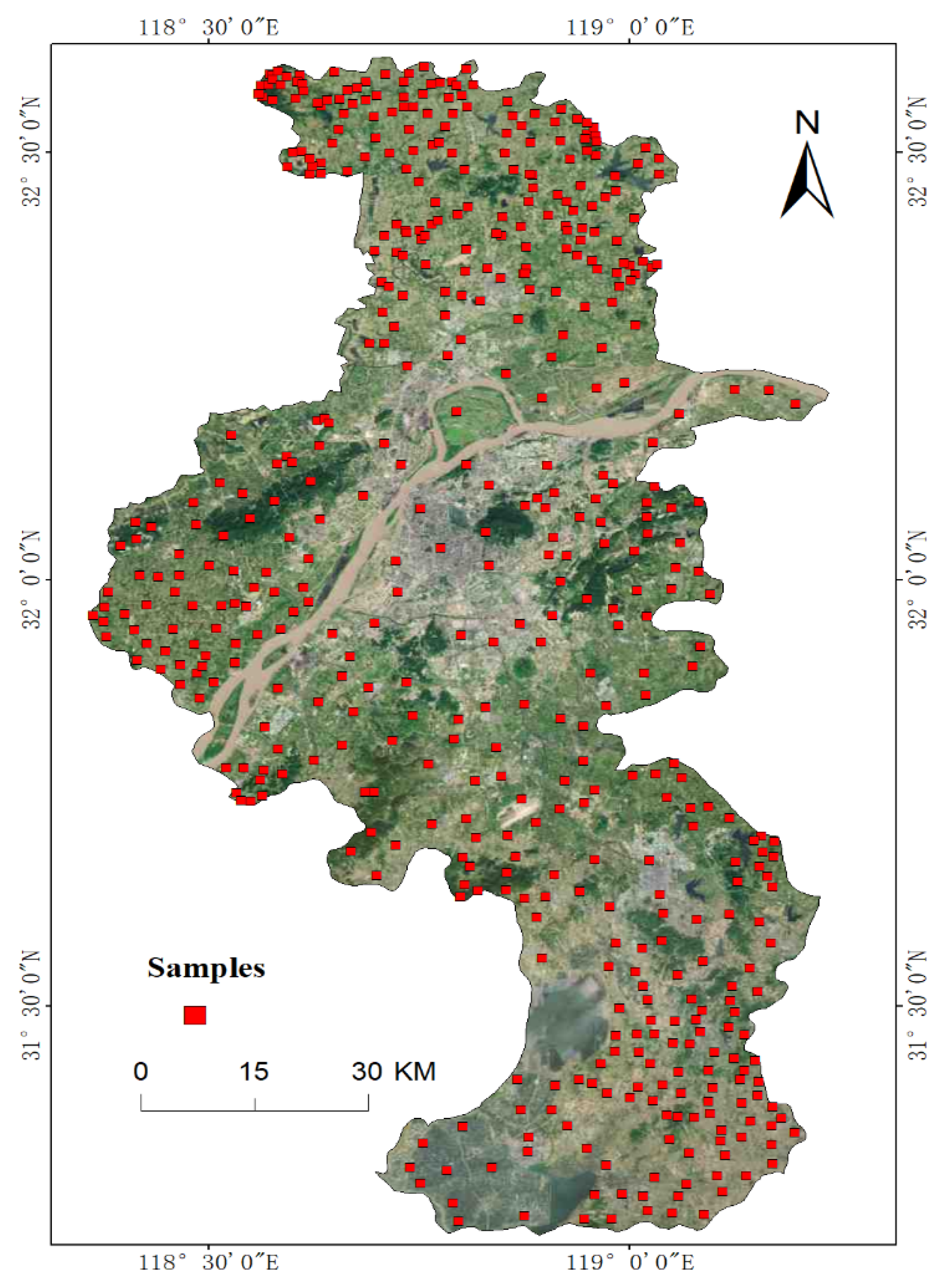
2.1. Study Area

The study area of Nanjing is located in southeastern China and southwestern Jiangsu Province, centered at latitude 32.06° N and longitude 118.80° E. The total land area is 6597 km2, and the distribution of major land-use types in Nanjing includes built-up areas, farmland, forest land, water, and grassland, as shown in Figure 1. The overall terrain of the region is relatively gentle, with a maximum elevation of about 300 m. The climate of Nanjing is a typical subtropical monsoon, with abundant precipitation (average annual precipitation: 1200 mm) and four distinct seasons. The average daily temperature ranges of summer and winter seasons in Nanjing are 20–29 °C and 2–11 °C, respectively [46]. As early as 2002, the Municipal Government made the strategic decision to build a “green Nanjing”. The goal was to build a modern urban greenspace, which was described as “landscape, urban and forest integration, ecological and economic win–win, harmonious human landscape, urban and rural coordination.” At present, the forest has become the most important resource in Nanjing, with ecology promotion as its biggest advantage. The urban tree coverage area has reached more than 31.2% of the total area (http://www.njyl.gov.cn/). Evergreen trees are an important part of the green ecological network system, due to their unique ecological and landscape aesthetic value. The evergreen tree species in Nanjing mainly include typical subtropical, evergreen broad-leaved tree species such as Magnolia, camphor, and evergreen coniferous trees (Pinus massoniana and yew). The highest proportion of evergreen shrub vegetation in Nanjing is Osmanthus.

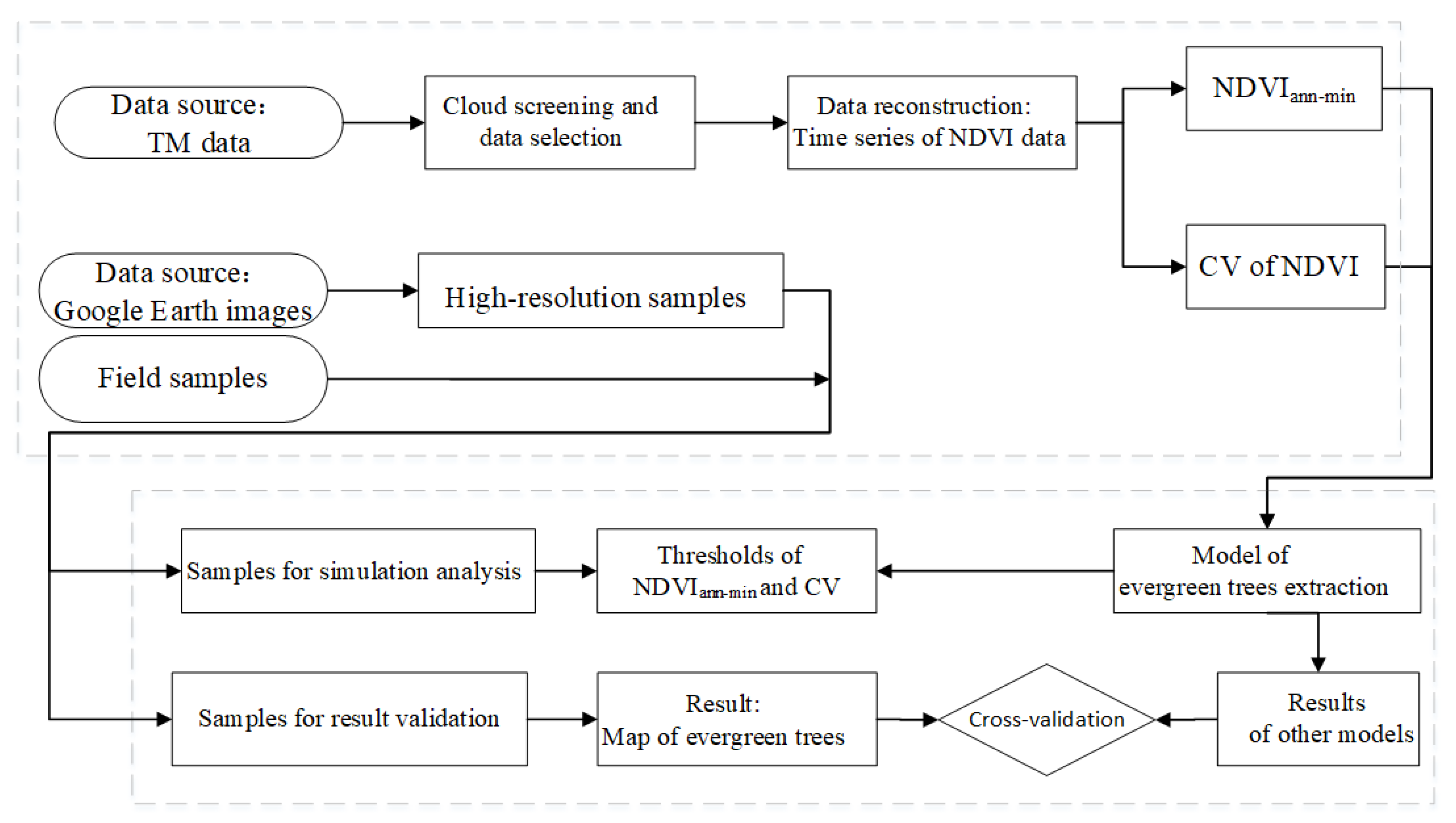
2.2. Methodology Flowchart

The detailed research process used in this study is shown in Figure 2. First, the remote-sensing images were preprocessed. The processed data were then used for model construction. The model was simulated with high-resolution imagery to determine a reasonable threshold for the parameters. Finally, the accuracy of the experimental results was evaluated to verify the feasibility of the method [47].

2.3. Data Selection and Reconstruction

Landsat 8 Thematic Mapper (TM) images (Path 120, row 38) for 2015–2017 with at least partially cloud-free imagery were downloaded from the United States Geological Survey Global Visualization Viewer website (http://glovis.usgs.gov/). Images acquired for this study were processed for atmospheric correction and geometric correction Level 2 T [48]. Twenty-four images constituted the original dataset, with a median of eight images per year (range: seven to 10 images per year). Two images were selected from each month (Table 1).
Nanjing is located in the subtropical zone, and is highly susceptible to precipitation, making it difficult to obtain continuous cloud-free images within a single year. During the three studied years (2015–2017), the spatial and temporal distribution of the urban green space remained virtually stable [49]. Thus, we assumed that the difference in vegetation coverage in the same month of different years (i.e., June 2015 and June 2017, September 2015 and September 2017, etc.) would be negligible, and used images obtained over three years to reconstruct the intra-year NDVI time-series dataset. The NDVI was calculated for each image date [(B5−B4)/(B5+B5)], which was originally developed by Rouse and applied by Tucker [50,51]. The maximum NDVI value was selected for two images in the same month, using the maximum value composites (MVC) method to minimize cloud shadow features [52]. The MVC method is an effective way of eliminating the undesirable influences of cloud cover, atmospheric constituents, and aerosol concentrations by retaining the highest value for each pixel location of several NDVI images [53]. Ultimately, we obtained 12 intra-annual continuous NDVI time-series images (one image per month). The time-series dataset was used to obtain the annual minimum NDVI (NDVIann-min) and CV values.

2.4. Evergreen Tree Extraction Model

The evergreen tree extraction model (NDVI-CV) consisted of two parts: the NDVIann-min and the CV of the NDVI time series. The CV reflects the degree of difference or dispersion of the overall unit marker values. The CV of the NDVI is the ratio of the standard deviation to the mean of the NDVI time series for each pixel. In a growth cycle, a smaller CV value for the NDVI time series indicates smoother seasonal fluctuations in the vegetation growth. The standard deviation of the time-series images σ and the average of the time-series images μ used to calculate the CV of a single pixel are given in Equations (1) and (2), respectively [45]:
σ = 1 n 1 [ m = 1 n ( N D V I ) m 2 ( m = 1 n N D V I m ) 2 ]
μ = m = 1 n ( N D V I ) m / n
where NDVIm is the NDVI value of image m, and n is the total number of images over the year. The CV calculation formula of the pixel for row i and column j is given by:
CoV i j = σ i j μ i j

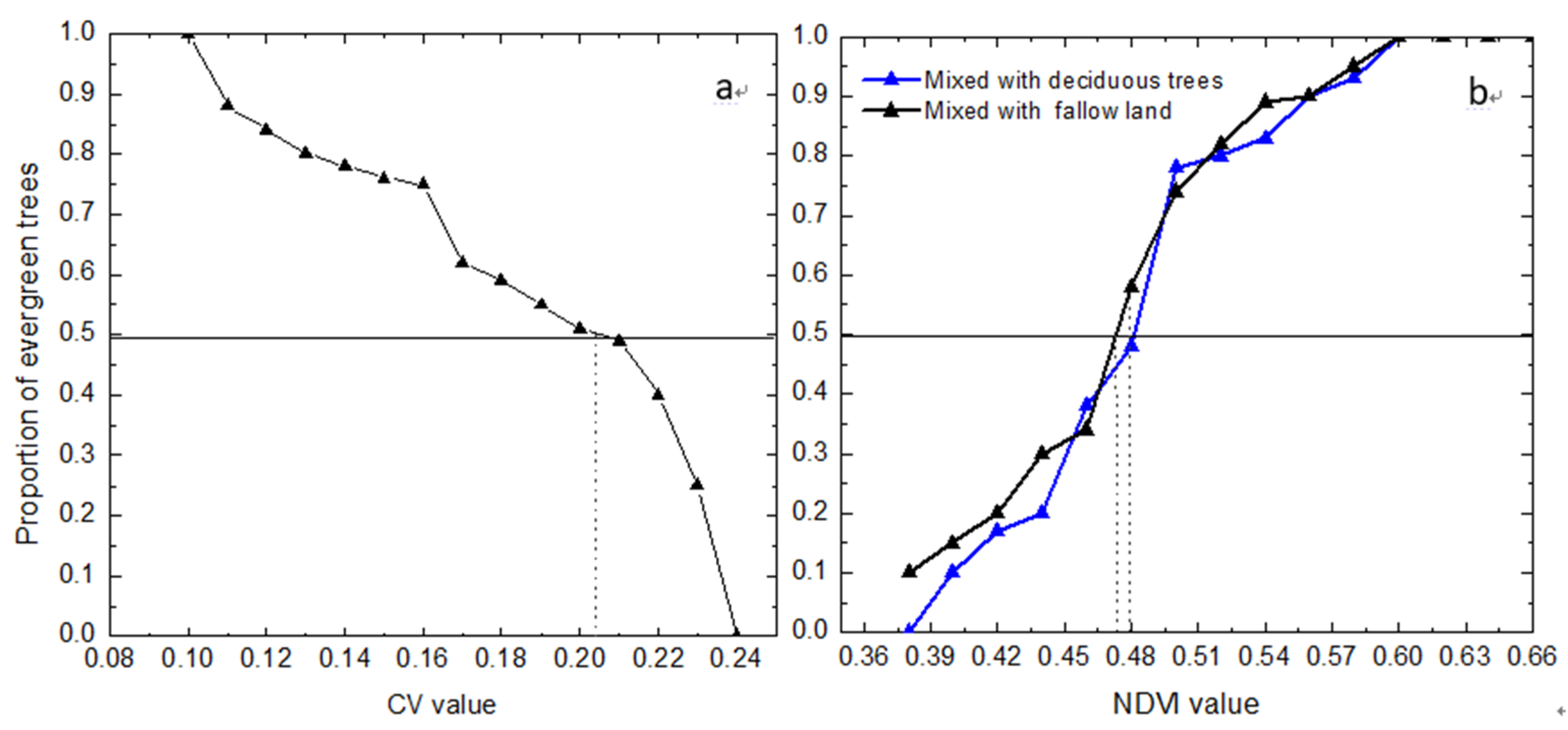
2.5. Model Threshold Analysis

The selection of reasonable NDVIann-min and CV thresholds are key steps in the proposed method [54]. Compared with the NDVI curves of deciduous trees, farmland, and mixed trees, evergreen trees are the most stable, with the smallest CV value (0.082). Moreover, evergreen trees had the highest NDVIann-min value, above 0.6, as shown in Figure 3. Combining the NDVIann-min and CV values to extract pure evergreen forest pixels was a relatively simple process. However, choosing reasonable CV and NDVIann-min thresholds for extracting evergreen trees from mixed pixels is difficult. For the purposes of simplifying the problem of mixed pixels, here we define a pixel (30 m × 30 m) as “evergreen trees” if the majority of its area (50% or greater) is covered by evergreen trees [55].
To extract evergreen trees in mixed pixels, the relationship between the CV value and the proportion of evergreen trees was analyzed, as shown in Table 2. In the mixed pixels of evergreen and deciduous trees, as the proportion of evergreen trees increases, the CV value decreases. However, the CV is invalid for distinguishing evergreen trees in the mixed pixels consisting of evergreen trees and fallow land, because of the close CV value of the two (Figure 3). Therefore, the constraint of NDVIann-min is necessary for extracting the evergreen trees in the mixed pixels of evergreen trees and fallow land.
The same analysis of the NDVIann-min threshold is shown in Table 3. NDVIann-min values of the mixed pixels varied with the different compositions in the pixel (i.e., composite of evergreen trees and deciduous trees or composite of evergreen trees and fallow land). As the proportion of evergreen trees changed, the change in the corresponding NDVIann-min value differed between mixed pixels of evergreen and deciduous trees (evergreen trees and fallow land). Therefore, the two cases were considered separately in the threshold analysis (Table 3). By analyzing the percentage of evergreen trees in mixed pixels, we estimated a preliminary CV value of <0.22 (Table 2) and an NDVIann-min value of ~0.48 (Table 3).
The percentage of evergreen trees within the pixel was validated by Google Earth high-resolution images and field sampling. In addition, we selected 1926 sample sites (50 m × 50 m) in the Google Earth images (Figure 4) and samples acquisition dates were shown in Table 4. 47 field samples based on a stratified random method to verify the accuracy of the models.

2.6. Comparative Analysis with Other Models

To verify the NDVI-CV model, a cross-comparison with the results of a previous model was performed. In other studies, the most widely used model to extract evergreen forests was the LSWI ((ρNIRρSWIR)/(ρNIR + ρSWIR)) [43,56]; evergreen forest information was determined based on the annual minimum LSWI threshold (LSWImin). The LSWI curve fluctuations of different types of vegetation during the growth cycle are similar to those of the NDVI. The LSWI curve of evergreen trees is relatively stable, whereas the LSWI curves of farmland and deciduous trees fluctuate greatly.
Furthermore, we also compared the NDVI-CV method with another two indexes derived from this paper: (1) the NDVIann-min evergreen tree extraction method (without CV constraints), and (2) the single NDVI image extraction method in winter, i.e., NDVIwin. In this study, the threshold of the methodology was consistent with the threshold of the NDVIann-min.

3. Results

3.1. Threshold Analysis Results

The relationship between a set of CV and NDVIann-min values and the proportion of the evergreen trees in mixed pixels was obtained (Figure 5). Parts of the CV and NDVIann-min values were selected and used in an example calculation (Table 2 and Table 3). The results showed that the proportion of evergreen trees gradually decreased with increasing CV values (Figure 5a), and increased with increasing NDVIann-min (Figure 5b) values. When the proportion of evergreen trees exceeded 0.5, the corresponding CV value should be <0.2. For mixed pixels formed by evergreen trees and deciduous trees or evergreen trees and fallow land, the same NDVI value corresponded to different evergreen tree ratios. Based on the simulation analysis results, the model CV threshold value should be <0.2, and the NDVIann-min should be >0.48. Using the same threshold analysis method, we determined that the threshold of LSWImin, based on the data in this paper, should be greater than 0.14.

3.2. Spatial Distribution of Evergreen Trees

Based on the threshold analysis, CV and NDVIann-min thresholds were obtained to extract the spatial distribution information of evergreen trees in Nanjing (Figure 6). The area of evergreen trees in Nanjing is 342.33 km2 according to the extraction result. Due to the green-space planning differences in different districts, the distribution of evergreen trees varies greatly from one district to another. Evergreen trees are mainly distributed in four districts of Nanjing: Jiangning, Pukou, Gaochun, and Lishui. The reason for this may be that these four districts include many hilly areas with concentrated trees. Therefore, the distribution of evergreen vegetation is relatively wide. By contrast, there are fewer evergreen trees in the central urban area and Liuhe District. In this case, the major land-use type in the central urban area is commercial or residential land, whereas evergreen trees exhibit a scattered distribution, making it more difficult to identify them. Additionally, due to its relatively flat terrain, Liuhe District tends to be a major crop-growing area.

3.3. Verification and Comparison of Models

We verified the classification accuracy of several models with Google Earth high-resolution images (Table 5). According to a confusion matrix [57], the overall classification accuracy of the NDVI-CV model was up to 93%; meanwhile, the user accuracy and producer precision [58] exceeded 92% and 85%, respectively. The classification accuracy of several models according to the field samples is described in Table 6. The overall classification accuracy of the NDVI-CV was 87%; this was the highest accuracy value among the models considered.
Compared with other models, NDVI-CV has the highest classification accuracy. Although the NDVIann-min and LSWImin are based on time-series methods, these two models extract evergreen trees by determining only the minimum value of the time series, which is still derived from a single image. Moreover, the NDVIwin model is derived from a single-phase image, whose classification accuracy can be predicted to be very low. In general, the NDVI-CV of a time series is more effective and stable.

4. Discussion

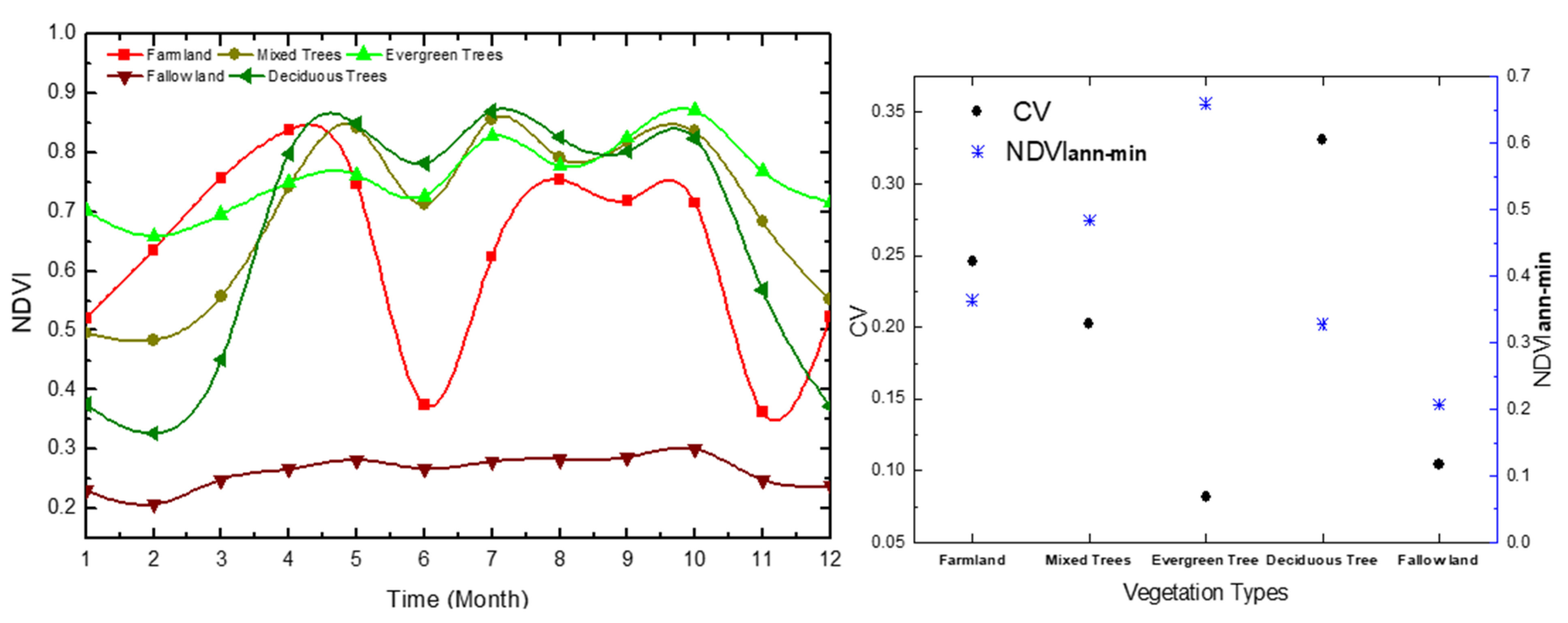
4.1. Analysis of Data on Phenology Characteristics of Evergreen Trees

The time-series classification method considers the characteristic phenology period of vegetation [59,60,61,62]. As shown above, the time-series NDVI-CV model achieved higher classification accuracy than the NDVIann-min, LSWImin, and NDVIwin. Unlike the NDVIann-min and LSWImin, which only select the best phase in the time series, or the NDVIwin model only that selects a single-phase image in winter, our new method considers multiple phenological features. Subtropical urban areas have complex vegetation types and severe fragmentation of land-use types. Therefore, it is necessary to reconstruct continuous, high-resolution data to extract vegetation information. In addition, compared with other vegetation types in subtropical zones (deciduous trees, grassland, farmland, etc.), changes in evergreen trees during the growth cycle are less affected by season and temperature, and growth fluctuations tend to be more stable. In a one-year period, the growth trend of evergreen trees and other vegetation could be distinguished.

4.2. Method Suitability

The CV is affected by changes in vegetation coverage, which depends on the CV formula itself. For example, some mixed pixels with a large proportion of deciduous trees showed relatively high NDVI values during the defoliation period. Neglecting the CV constraint would cause the misclassification of such pixels as evergreen trees, because the NDVIann-min value was greater than the threshold. NDVI is the most sensitive to moderate vegetation coverage. Thus, when the proportion of fallow land is about 50%, the classification accuracy of the NDVI is the highest for mixed pixels of evergreen trees and fallow land [63]. In the cross-validation comparison, although the classification accuracy of NDVIann-min showed little difference to the accuracy of the NDVI-CV model, this method still has certain deficiencies. It would generate different results for other study areas with different vegetation coverage characteristics. This is due to the variation in the sensitivity of the NDVI according to different vegetation coverage types. Moreover, as NDVIann-min is a phenological node of the time-series, it omits some important phenology characteristics.
The NDVI-CV model is more stable for evergreen species whose leaf color is greatly affected by moisture content compared with LSWImin [64,65]. Figure 7a shows a false color image of the Landsat 6/5/4 band synthesis, which is used to enhance the vegetation area. The image was taken on 9 February 2016 (in winter). The red square is generated by the image processing software; the difference between the extraction results of the two models is more obvious in the red square (Figure 7). Comparing the NDVI-CV method with the LSWImin method, the color of the forest within the red-framed area was slightly brighter than that of the surrounding forest. The NDVI-CV method extracted this information successfully, whereas the LSWImin method misclassified this area as other vegetation. This is because the leaf moisture content of evergreen species is affected by season, and because the LSWI is more sensitive to leaf water content variations [56,66].
The continuous time-series advantage of the NDVI-CV model effectively avoided the interference of other vegetation with similar spectral characteristics as that of forest land. In previous research on vegetation extraction, the key phenological phase of a particular vegetation that is different from other land-use types was first determined; then, the vegetation information was extracted using a single image or several images during the key phenological phase. The key phenological phase of evergreen trees in the study area is from December to February of the following year. For this period, the NDVI values of most of the deciduous trees and grasslands are at annual minima. However, some crops undergo a growth stage during this period, and the associated NDVI values of these crops are high (Figure 8). Therefore, using a single image does not avoid spectral confusion among multiple vegetation types with similar spectral features, whereas the continuous time-series NDVI-CV model shows better classification results.

4.3. Limitations and Deficiencies

Landsat images have limited high-quality data in subtropical rainy regions, resulting in intra-annual time-series with unequal, long (~one month) intervals during a year. The shorter the time-series interval, the closer the NDVI curves are to vegetation growth fluctuations. The NDVIann-min threshold may be biased due to a lack of data for some key nodes. Reducing the intervals of the time series can improve the stability of the model and increase the precision. In addition, although the land-use dynamics in the research area remained basically stable over the three-year study period, there were still inevitable changes that may have led to classification errors.
Future studies should work toward a more accurate acquisition of evergreen forest information from mixed pixels. Additionally, the optimization of the NDVI-CV model relies on the use of remote-sensing images with enhanced spatiotemporal resolution.

5. Conclusions

In this work, we used cloud-free and partially cloud-free Landsat remote-sensing images acquired over three years to reconstruct an intra-annual continuous time-series dataset for evergreen tree extraction. Our method combines the NDVIann-min with the CV. The results indicated that the proposed method accurately identified evergreen trees. In a subtropical urban area with complex and fragmented land-use types, the proposed model effectively avoided spectral confusion between evergreen trees and other vegetation, such as forest plantation and farmland, by reducing the interference of mixed pixels in the extraction results. Using Google Earth high-resolution images to verify the model, the user accuracy, producer accuracy, and overall accuracy of the model were high, at 92.3%, 85.2%, and 93%, respectively. The total accuracy of field sampling verification also exceeded 87%. Therefore, the NDVI-CV model of time-series is a more stable and accurate. Future research should address the means to obtain continuous inter-annual time-series data and the real-time monitoring of changes in the spatiotemporal distribution of evergreen trees.

Author Contributions

Y.Y. designed and conducted the experiments and wrote the manuscript. T.W. and S.W. provided suggestions for the idea, data analysis, discussion, and manuscript writing. F.M. and J.L. modified the expression and grammar of the manuscript.

Funding

This research was funded by the Fundamental Research Funds for the Central Universities (grant no. 2017B05114, 2017B20514), National Science Foundation of China (grant no. 41371359, 41671362) and the Major Special Project—the China High-Resolution Earth Observation System (30-Y30B13-9003-14/16).

Acknowledgments

This work was supported by the Fundamental Research Funds for the Central Universities (grant no. 2017B05114, 2017B20514), National Science Foundation of China (grant no. 41371359, 41671362) and the Major Special Project—the China High-Resolution Earth Observation System (30-Y30B13-9003-14/16) supported this research.

Conflicts of Interest

The authors declare no conflict of interest.

References

  1. Dong, J.; Xiao, X.; Sheldon, S.; Biradar, C.; Xie, G. Mapping tropical forests and rubber plantations in complex landscapes by integrating PALSAR and MODIS imagery. ISPRS J. Photogramm. Remote. Sens. 2012, 74, 20–33. [Google Scholar] [CrossRef]
  2. Wang, H.; Shi, H.; Li, Y. Leaf dust capturing capacity of urban greening plant species in relation to leaf micromorphology. In Proceedings of the 2011 International Symposium on Water Resource and Environmental Protection, Xi’an, China, 20–22 May 2011; pp. 2198–2201. [Google Scholar]
  3. Shi, H.; Qin, Q.; Liao, J.; Chen, G.; Ding, Z. Study on carbon fixation and oxygen release capabilities of 10 dominant garden plants in Wuhan city. J. Cent. South Univ. For. Technol. 2011, 31, 87–90. (In Chinese) [Google Scholar]
  4. Zhang, Z.; Lv, Y.; Pan, H. Cooling and humidifying effect of plant communities in subtropical urban parks. Urban For. Urban Green. 2013, 12, 323–329. [Google Scholar] [CrossRef]
  5. Yoder, B.J.; Ryan, M.G.; Waring, R.H.; Schoettle, A.W.; Kaufmann, M.R. Evidence of Reduced Photosynthetic Rates in Old Trees. For. Sci. 1994, 40, 513–527. [Google Scholar] [CrossRef]
  6. Zhuang, Z.; Hongyan, Z. Study on Path Dependence and Innovation of the Governance System Changes in State-owned Forest Regions in China. For. Econ. 2018, 8. (In Chinese) [Google Scholar] [CrossRef]
  7. Gabler, K.; Schadauer, K. Some approaches and designs of sample-based national forest inventories. Austrian J. For. Sci. 2007, 124, 105–133. [Google Scholar]
  8. Xie, Y.; Sha, Z.; Yu, M. Remote sensing imagery in vegetation mapping: A review. J. Plant. Ecol. 2008, 1, 9–23. [Google Scholar] [CrossRef]
  9. Sannier, C.; McRoberts, R.E.; Fichet, L.-V.; Makaga, E.M.K. Using the regression estimator with Landsat data to estimate proportion forest cover and net proportion deforestation in Gabon. Remote Sens. Environ. 2014, 151, 138–148. [Google Scholar] [CrossRef]
  10. Estoque, R.C.; Murayama, Y. Classification and change detection of built-up lands from Landsat-7 ETM+ and Landsat-8 OLI/TIRS imageries: A comparative assessment of various spectral indices. Ecol. Indic. 2015, 56, 205–217. [Google Scholar] [CrossRef]
  11. Bolton, D.K.; Friedl, M.A. Forecasting crop yield using remotely sensed vegetation indices and crop phenology metrics. Agric. For. Meteorol. 2013, 173, 74–84. [Google Scholar] [CrossRef]
  12. Boryan, C.; Yang, Z.; Mueller, R.; Craig, M. Monitoring US agriculture: The US Department of Agriculture, National Agricultural Statistics Service, Cropland Data Layer Program. Geocarto Int. 2011, 26, 341–358. [Google Scholar] [CrossRef]
  13. Funk, C.; Budde, M.E. Phenologically-tuned MODIS NDVI-based production anomaly estimates for Zimbabwe. Remote Sens. Environ. 2009, 113, 115–125. [Google Scholar] [CrossRef]
  14. Huang, C.; Goward, S.N.; Schleeweis, K.; Thomas, N.; Masek, J.G.; Zhu, Z. Dynamics of national forests assessed using the Landsat record: Case studies in eastern United States. Remote Sens. Environ. 2009, 113, 1430–1442. [Google Scholar] [CrossRef]
  15. Sakamoto, T.; Gitelson, A.A.; Arkebauer, T.J. MODIS-based corn grain yield estimation model incorporating crop phenology information. Remote Sens. Environ. 2013, 131, 215–231. [Google Scholar] [CrossRef]
  16. Van Niel, T.G.; McVicar, T.R. Determining temporal windows for crop discrimination with remote sensing: A case study in south-eastern Australia. Comput. Electron. Agric. 2004, 45, 91–108. [Google Scholar] [CrossRef]
  17. Yang, C.; Everitt, J.H.; Murden, D. Evaluating high resolution SPOT 5 satellite imagery for crop identification. Comput. Electron. Agric. 2011, 75, 347–354. [Google Scholar] [CrossRef]
  18. Immitzer, M.; Vuolo, F.; Atzberger, C. First Experience with Sentinel-2 Data for Crop and Tree Species Classifications in Central Europe. Remote Sens. 2016, 8, 166. [Google Scholar] [CrossRef]
  19. Lo, C.P.; Choi, J. A hybrid approach to urban land use/cover mapping using Landsat 7 Enhanced Thematic Mapper Plus (ETM+) images. Int. J. Remote Sens. 2004, 25, 2687–2700. [Google Scholar] [CrossRef]
  20. Yuan, H.; Van Der Wiele, C.F.; Khorram, S. An Automated Artificial Neural Network System for Land Use/Land Cover Classification from Landsat TM Imagery. Remote Sens. 2009, 1, 243–265. [Google Scholar] [CrossRef]
  21. Peña, M.; Brenning, A. Assessing fruit-tree crop classification from Landsat-8 time series for the Maipo Valley, Chile. Remote Sens. Environ. 2015, 171, 234–244. [Google Scholar] [CrossRef]
  22. Chang, J.; Hansen, M.C.; Pittman, K.; Carroll, M.; DiMiceli, C. Corn and soybean mapping in the united states using MODN time-series data sets. Agron. J. 2007, 99, 1654–1664. [Google Scholar] [CrossRef]
  23. Foerster, S.; Kaden, K.; Foerster, M.; Itzerott, S. Crop type mapping using spectral–temporal profiles and phenological information. Comput. Electron. Agric. 2012, 89, 30–40. [Google Scholar] [CrossRef]
  24. Graesser, J.; Ramankutty, N. Detection of cropland field parcels from Landsat imagery. Remote Sens. Environ. 2017, 201, 165–180. [Google Scholar] [CrossRef]
  25. Huang, H.; Chen, Y.; Clinton, N.; Wang, J.; Wang, X.; Liu, C.; Gong, P.; Yang, J.; Bai, Y.; Zheng, Y.; et al. Mapping major land cover dynamics in Beijing using all Landsat images in Google Earth Engine. Remote Sens. Environ. 2017, 202, 166–176. [Google Scholar] [CrossRef]
  26. Mertes, C.; Schneider, A.; Sulla-Menashe, D.; Tatem, A.; Tan, B. Detecting change in urban areas at continental scales with MODIS data. Remote Sens. Environ. 2015, 158, 331–347. [Google Scholar] [CrossRef]
  27. Moreau, I.; Defourny, P. The vegetation phenology detection in Amazon tropical evergreen forests using SPOT-VEGETATION 11-y time series. In Proceedings of the 2012 IEEE International Geoscience and Remote Sensing Symposium, Munich, Germany, 22–27 July 2012; pp. 40–43. [Google Scholar]
  28. Potapov, P.V.; Turubanova, S.A.; Hansen, M.C.; Adusei, B.; Broich, M.; Altstatt, A.; Mané, L.; Justice, C.O. Quantifying forest cover loss in Democratic Republic of the Congo, 2000–2010, with Landsat ETM+ data. Remote Sens. Environ. 2012, 122, 106–116. [Google Scholar] [CrossRef]
  29. Senf, C.; Pflugmacher, D.; Van Der Linden, S.; Hostert, P. Mapping Rubber Plantations and Natural Forests in Xishuangbanna (Southwest China) Using Multi-Spectral Phenological Metrics from MODIS Time Series. Remote Sens. 2013, 5, 2795–2812. [Google Scholar] [CrossRef]
  30. Bush, R.; Markakis, J. Zimbabwe out in the cold? Rev. Afri. Polit. Econ. 2003, 30, 535–537. [Google Scholar] [CrossRef]
  31. Wardlow, B.; Egbert, S.; Kastens, J. Analysis of time-series MODIS 250 m vegetation index data for crop classification in the U.S. Central Great Plains. Remote Sens. Environ. 2007, 108, 290–310. [Google Scholar] [CrossRef]
  32. Zeng, L.; Wardlow, B.D.; Wang, R.; Shan, J.; Tadesse, T.; Hayes, M.J.; Li, D. A hybrid approach for detecting corn and soybean phenology with time-series MODIS data. Remote Sens. Environ. 2016, 181, 237–250. [Google Scholar] [CrossRef]
  33. Healey, S.P.; Cohen, W.B.; Spies, T.A.; Moeur, M.; Pflugmacher, D.; Whitley, M.G.; Lefsky, M.; et al. The Relative Impact of Harvest and Fire upon Landscape-Level Dynamics of Older Forests: Lessons from the Northwest Forest Plan. Ecosystems 2008, 11, 1106–1119. [Google Scholar] [CrossRef]
  34. Masek, J.G.; Huang, C.; Wolfe, R.; Cohen, W.; Hall, F.; Kutler, J.; Nelson, P. North American forest disturbance mapped from a decadal Landsat record. Remote Sens. Environ. 2008, 112, 2914–2926. [Google Scholar] [CrossRef]
  35. Cai, Y.; Guan, K.; Peng, J.; Wang, S.; Seifert, C.; Wardlow, B.; Li, Z. A high-performance and in-season classification system of field-level crop types using time-series Landsat data and a machine learning approach. Remote Sens. Environ. 2018, 210, 35–47. [Google Scholar] [CrossRef]
  36. Gao, F.; Hilker, T.; Zhu, X.; Anderson, M.; Masek, J.; Wang, P.; Yang, Y. Fusing Landsat and MODIS Data for Vegetation Monitoring. IEEE Geosci. Remote Sens. 2015, 3, 47–60. [Google Scholar] [CrossRef]
  37. Gao, F.; Wang, P.; Masek, J.; et al. Integrating remote sensing data from multiple optical sensors for ecological and crop condition monitoring. Remote Sens. Model. Ecosyst. Sustain. 2013, 869, 886903. [Google Scholar] [CrossRef]
  38. Gamon, J.A.; Field, C.B.; Goulden, M.L.; Griffin, K.L.; Hartley, A.E.; Joel, G.; Peñuelas, J.; Valentini, R. Relationships Between NDVI, Canopy Structure, and Photosynthesis in Three Californian Vegetation Types. Ecol. Appl. 1995, 5, 28–41. [Google Scholar] [CrossRef]
  39. Kou, W.; Liang, C.; Wei, L.; Hernandez, A.J.; Yang, X.; et al. Phenology-Based Method for Mapping Tropical Evergreen Forests by Integrating of MODIS and Landsat Imagery. Forests 2017, 8, 34. [Google Scholar] [CrossRef]
  40. Qin, Y.; Xiao, X.; Dong, J.; Zhang, G.; Roy, P.S.; Joshi, P.K.; Gilani, H.; Murthy, M.S.R.; Jin, C.; Wang, J.; et al. Mapping forests in monsoon Asia with ALOS PALSAR 50-m mosaic images and MODIS imagery in 2010. Sci. Rep. 2016, 6. [Google Scholar] [CrossRef]
  41. Xiao, X.; Boles, S.; Liu, J.; Zhuang, D.; Frolking, S.; Li, C.; Salas, W.; Moore, B. Mapping paddy rice agriculture in southern China using multi-temporal MODIS images. Remote Sens. Environ. 2005, 95, 480–492. [Google Scholar] [CrossRef]
  42. Xiao, X.; Boles, S.; Liu, J.; Zhuang, D.; Liu, M. Characterization of forest types in Northeastern China, using multi-temporal SPOT-4 VEGETATION sensor data. Remote Sens. Environ. 2002, 82, 335–348. [Google Scholar] [CrossRef]
  43. Xiao, X.; Biradar, C.M.; Czarnecki, C.; Alabi, T.; Keller, M. A Simple Algorithm for Large-Scale Mapping of Evergreen Forests in Tropical America, Africa and Asia. Remote Sens. 2009, 1, 355–374. [Google Scholar] [CrossRef]
  44. Melaas, E.K.; Friedl, M.A.; Zhu, Z. Detecting interannual variation in deciduous broadleaf forest phenology using Landsat TM/ETM+ data. Remote Sens. Environ. 2013, 132, 176–185. [Google Scholar] [CrossRef]
  45. Weiss, E.; Marsh, S.E.; Pfirman, E.S. Application of NOAA-AVHRR NDVI time-series data to assess changes in Saudi Arabia’s rangelands. Int. J. Remote Sens. 2001, 22, 1005–1027. [Google Scholar] [CrossRef]
  46. Liu, G.; Zhang, Q.; Li, G.; Doronzo, D.M. Response of land cover types to land surface temperature derived from Landsat-5 TM in Nanjing Metropolitan Region, China. Environ. Geol. 2016, 75, 1386. [Google Scholar] [CrossRef]
  47. Li, P.; Jiang, L.; Feng, Z. Cross-Comparison of Vegetation Indices Derived from Landsat-7 Enhanced Thematic Mapper Plus (ETM+) and Landsat-8 Operational Land Imager (OLI) Sensors. Remote Sens. 2013, 6, 310–329. [Google Scholar] [CrossRef]
  48. Richter, R. A spatially adaptive fast atmospheric correction algorithm. Int. J. Remote Sens. 1996, 17, 1201–1214. [Google Scholar] [CrossRef]
  49. Chen, J.; Gao, J.; Chen, W. Urban land expansion and the transitional mechanisms in Nanjing, China. Habitat Int. 2016, 53, 274–283. [Google Scholar] [CrossRef]
  50. Rouse, J.J.W.; Haas, R.H.; Schell, J.A.; Deering, D.W. Monitoring Vegetation Systems in the Great Plains with ERTS. Available online: https://ntrs.nasa.gov/archive/nasa/casi.ntrs.nasa.gov/19740022614.pdf (accessed on 5 February 2019).
  51. Tucker, C.J. Red and photographic infrared linear combinations for monitoring vegetation. Remote Sens. Environ. 1979, 8, 127–150. [Google Scholar] [CrossRef]
  52. Marcal, A.R.S.; Wright, G.G. The use of ‘overlapping’ NOAA-AVHRR NDVI maximum value composites for Scotland and initial comparisons with the land cover census on a Scottish Regional and District basis. Int. J. Remote Sens. 1997, 18, 491–503. [Google Scholar] [CrossRef]
  53. Holben, B.N. Characteristics of maximum-value composite images from temporal AVHRR data. Int. J. Remote Sens. 1986, 7, 1417–1434. [Google Scholar] [CrossRef]
  54. Maxwell, S.K.; Sylvester, K.M. Identification of “ever-cropped” land (1984–2010) using Landsat annual maximum NDVI image composites: Southwestern Kansas case study. Remote Sens. Environ. 2012, 121, 186–195. [Google Scholar] [CrossRef] [PubMed]
  55. Goldblatt, R.; Stuhlmacher, M.F.; Tellman, B.; Clinton, N.; Hanson, G.; Georgescu, M.; Wang, C.; Serrano-Candela, F.; Khandelwal, A.K.; Cheng, W.-H.; et al. Using Landsat and nighttime lights for supervised pixel-based image classification of urban land cover. Remote Sens. Environ. 2018, 205, 253–275. [Google Scholar] [CrossRef]
  56. Chandrasekar, K.; Sai, M.V.R.S.; Roy, P.S.; Dwevedi, R.S. Land Surface Water Index (LSWI) response to rainfall and NDVI using the MODIS Vegetation Index product. Int. J. Remote Sens. 2010, 31, 3987–4005. [Google Scholar] [CrossRef]
  57. Lucas, I.; Janssen, F.; van der Wel, F.J. Accuracy assessment of satellite derived land cover data: A review. Photogramm. Eng. Remote Sens. 1994, 60, 419–426. [Google Scholar]
  58. Story, M.; Congalton, R.G. Accuracy assessment: A user’s perspective. Photogramm. Eng. Remote Sens. 1986, 52, 397–399. [Google Scholar]
  59. Cohen, W.B.; Yang, Z.; Kennedy, R. Detecting trends in forest disturbance and recovery using yearly Landsat time series: 2. TimeSync—Tools for calibration and validation. Remote Sens. Environ. 2010, 114, 2911–2924. [Google Scholar] [CrossRef]
  60. Ju, J.; Masek, J.G. The vegetation greenness trend in Canada and US Alaska from 1984–2012 Landsat data. Remote Sens. Environ. 2016, 176, 1–16. [Google Scholar] [CrossRef]
  61. Kim, D.-H.; Sexton, J.O.; Noojipady, P.; Huang, C.; Anand, A.; Channan, S.; Feng, M.; Townshend, J.R. Global, Landsat-based forest-cover change from 1990 to 2000. Remote Sens. Environ. 2014, 155, 178–193. [Google Scholar] [CrossRef]
  62. Sakamoto, T.; Yokozawa, M.; Toritani, H.; Shibayama, M.; Ishitsuka, N.; Ohno, H. A crop phenology detection method using time-series MODIS data. Remote Sens. Environ. 2005, 96, 366–374. [Google Scholar] [CrossRef]
  63. Yoshioka, H. Analysis of Vegetation Isolines in Red-NIR Reflectance Space. Remote Sens. Environ. 2000, 74, 313–326. [Google Scholar] [CrossRef]
  64. Alberti, M. Maintaining ecological integrity and sustaining ecosystem function in urban areas. Curr. Opin. Environ. Sustain. 2010, 2, 178–184. [Google Scholar] [CrossRef]
  65. Carlson, T.N.; Ripley, D.A. On the relation between NDVI, fractional vegetation cover, and leaf area index. Remote Sens. Environ. 1997, 62, 241–252. [Google Scholar] [CrossRef]
  66. Jurgens, C. The modified normalized difference vegetation index (mNDVI) a new index to determine frost damages in agriculture based on Landsat TM data. Int. J. Remote Sens. 1997, 18, 3583–3594. [Google Scholar] [CrossRef]
Figure 1. Location of the study area showing the land-use types obtained from GlobeLand 30 in 2010.
Forests 10 00139 g001
Figure 2. Flowchart of subtropical evergreen tree mapping and accuracy assessment. TM = Thematic Mapper; NDVI = normalized difference vegetation index; CV = coefficient of variation.
Forests 10 00139 g002
Figure 3. Different vegetation pixels of the time-series variation of Landsat 8-derived normalized difference vegetation index (NDVI) curves (left), and the coefficient of variation (CV) value and annual minimum NDVI (NDVIann-min) value corresponding to each curve (right).
Forests 10 00139 g003
Figure 4. Partial samples in the Google Earth images.
Forests 10 00139 g004
Figure 5. Model threshold analysis results: variation in proportion of evergreen trees with changes in (a) the CV in mixed pixels of evergreen trees and deciduous trees, and (b) the NDVI in two types of mixed pixels composed of evergreen trees and another vegetation type.
Forests 10 00139 g005
Figure 6. Spatial distribution of evergreen trees in Nanjing.
Forests 10 00139 g006
Figure 7. Comparison of maps with the 30-m Landsat 8 Thematic Mapper (TM) image on 9 February 2016. (a) Evergreen trees appear as green on composite Landsat 8 TM images combined as false color (6/5/4). (b) Subtropical evergreen trees in the study area based on the NDVI-CV model. (c) Map of the LSWImin model.
Forests 10 00139 g007
Figure 8. Farmland grown in single-phase images in winter: (a) 30-m Landsat 8 Thematic Mapper (TM) image combined as false color (6/5/4) on 9 February 2016, and (b) farmland most likely extracted as evergreen vegetation.
Forests 10 00139 g008
Table 1. Acquisition dates of Landsat 8 images.
YearImage Acquisition Date
201521 January 13 May14 June
2016 9 February28 March13 April
29 April
201726 January27 February15 March 18 May3 June
2015 17 August2 September20 October5 November
2016 20 September 9 December
20175 July6 August 9 October26 November12 December
21 July
Table 2. Relationship between the coefficient of variation (CV) and the weight of evergreen trees in corresponding pixels. The CV value changes as the proportion of evergreen trees in the pixel changes.
CV Value0.100.130.160.190.22
ProportionEvergreen trees10.800.750.550.40
Deciduous trees00.200.250.450.50
Table 3. Relationship between the annual minimum normalized difference vegetation index (NDVIann-min) and proportion of evergreen trees in corresponding mixed pixels. The NDVIann-min value changes as the proportion of evergreen trees in the pixel changes.
NDVIann-min Value0.400.440.480.520.56
ProportionEvergreen trees0.10.20.50.80.9
Deciduous trees0.90.80.50.20.1
Evergreen trees0.150.30.60.80.9
Fallow land0.850.70.40.20.1
Table 4. Acquisition dates of samples.
Sampling dateSamples in Google Earth imagesField samples
December 2016February 2017July 2017October 2017April 2018
Table 5. Comparison of high-resolution image verification accuracy. LSWI: land surface water index.
ModelClass (pixels)Evergreen TreesOthersProducer Accuracy
NDVI-CVEvergreen trees5654792.3%
Others98122693.3%
User accuracy85.2%96.3%Overall accuracy
93.0%
LSWIminEvergreen trees47114176.9%
Others209110584.1%
User accuracy80.0%81.5%Overall accuracy
80.8%
NDVIann-minEvergreen trees5407288.2%
Others117314189.3%
User accuracy82.7%93.7%Overall accuracy
90.0%
NDVIwinEvergreen trees41719568.2%
Others77054458.6%
User accuracy68.1%58.8%Overall accuracy
64.1%
Table 6. Field sampling accuracy assessment.
ModelCV-NDVILSWIminNDVIann-minNDVIwin
Total classification accuracy87%65%83%56%

