Article

Species Diversity Associated with Foundation Species in Temperate and Tropical Forests

1
Harvard Forest, Harvard University, Petersham, MA 01366, USA
2
School of Science, Auckland University of Technology, Auckland Central 1010, New Zealand
3
Instituto Amazónico de Investigaciones Científicas Sinchi, Leticia, Colombia
4
Universidad Nacional de Colombia Sede Medellín, Medelliín, Colombia
5
S.J. & Jessie E. Quinney College of Natural Resources and the Ecology Center, Utah State University, Logan, UT 84322, USA
6
Department of Biology, Washington University in St. Louis, Saint Louis, MO 63130, USA
7
Department of Environmental Sciences, University of Puerto Rico–Rio Piedras, Rio Piedras 00925, Puerto Rico
*
Author to whom correspondence should be addressed.
Forests 2019, 10(2), 128; https://doi.org/10.3390/f10020128
Submission received: 11 January 2019 / Revised: 2 February 2019 / Accepted: 4 February 2019 / Published: 5 February 2019
(This article belongs to the Special Issue Causes and Consequences of Species Diversity in Forest Ecosystems)

Abstract

:
Foundation species define and structure ecological communities but are difficult to identify before they are declining. Yet, their defining role in ecosystems suggests they should be a high priority for protection and management while they are still common and abundant. We used comparative analyses of six large forest dynamics plots spanning a temperate-to-tropical gradient in the Western Hemisphere to identify statistical “fingerprints” of potential foundation species based on their size-frequency and abundance-diameter distributions, and their spatial association with five measures of diversity of associated woody plant species. Potential foundation species are outliers from the common “reverse-J” size-frequency distribution, and have negative effects on alpha diversity and positive effects on beta diversity at most spatial lags and directions. Potential foundation species also are more likely in temperate forests, but foundational species groups may occur in tropical forests. As foundation species (or species groups) decline, associated landscape-scale (beta) diversity is likely to decline along with them. Preservation of this component of biodiversity may be the most important consequence of protecting foundation species while they are still common.

1. Introduction

Foundation species (sensu [1,2]) define and structure ecological communities and entire ecosystems through bottom-up control of species diversity and non-trophic modulation of energy and nutrient cycles [3]. Foundation species tend to be common and abundant and generally receive less attention from ecologists, regulatory agencies, or conservation biologists who are otherwise focused on the study, management or protection of rare, threatened, or endangered species [4,5]. However, because foundation species are likely to control the distribution and abundance of such rare species, it has been argued that foundation species should be protected before their populations decline to non-functional levels or disappear entirely [6].
Identification of foundation species, however, is challenging. It can take many years—often decades—to acquire sufficient data to distinguish foundation species from species that also are common or abundant but lack “foundational” characteristics. In part, this is because the non-trophic effects of foundation species [3] usually are more subtle and harder to detect than trophic (“who-eats-whom”) interactions characteristic of keystone species (sensu [7,8]) or competitive interactions characteristic of “dominant” (sensu [9]) species. If indeed we are in the midst of Earth’s sixth mass extinction [10], it is imperative to prioritize the identification—and subsequent protection—of foundation species because of the unique role they play in structuring diversity of associated species at a range of spatial scales.
Data from networks of observations and experiments focused on species distributions and interactions (e.g., [11,12,13,14]) provide an opportunity to use specific statistical criteria to sieve large numbers of species for candidate foundation species. Because one characteristic of foundation species is that they control the diversity of associated species, we would predict that either the number of species (species richness) or measures of diversity weighted by the abundance of individual species would differ between plots that differ in size or abundance of foundation species [15]. We note that there is no explicit or implicit magnitude or directionality of the effect of a foundation species on associated diversity, but that foundational tree species tend to have lower species richness of associated plants whereas foundational herbaceous species tend to have higher species richness of associated plants [15]. Concomitantly, between-plot (beta) diversity is generally enhanced by the size or abundance of foundation species [15].
Here, we leverage our knowledge that Tsuga canadensis (eastern hemlock) is a foundation species in eastern North American forests [16] to explore whether statistical patterns of its abundance, size, and effects on associated diversity of woody plant species in the large (35-ha) forest dynamics plot at Harvard Forest have analogs among species in other large forest dynamics plots elsewhere in the Western Hemisphere. The myriad foundational roles of Tsuga canadensis have been documented by over a century of research [17], and it was the species that was first used to characterize foundation tree species [2]. The effects of T. canadensis on associated species and the forest ecosystems they create [15,16,18] also are similar to those of other dominant forest species since revealed as foundation species [6].
For this study, we first identified candidate foundation species (henceforth “focal species”) in five other forests across a temperate-to-tropical latitudinal gradient by comparing their size-frequency and diameter-abundance distributions with those observed for T. canadensis at Harvard Forest. We then used codispersion analysis [19] to explore positive and negative spatial associations between foundation species and the diversity of co-occurring woody taxa. Codispersion analysis has been used previously in forest ecology to explore patterns and processes in pairwise species co-occurrences [20], relationships between species occurrences and underlying environmental gradients [21], and temporal changes in spatial patterns of species abundances [22,23].

2. Materials and Methods

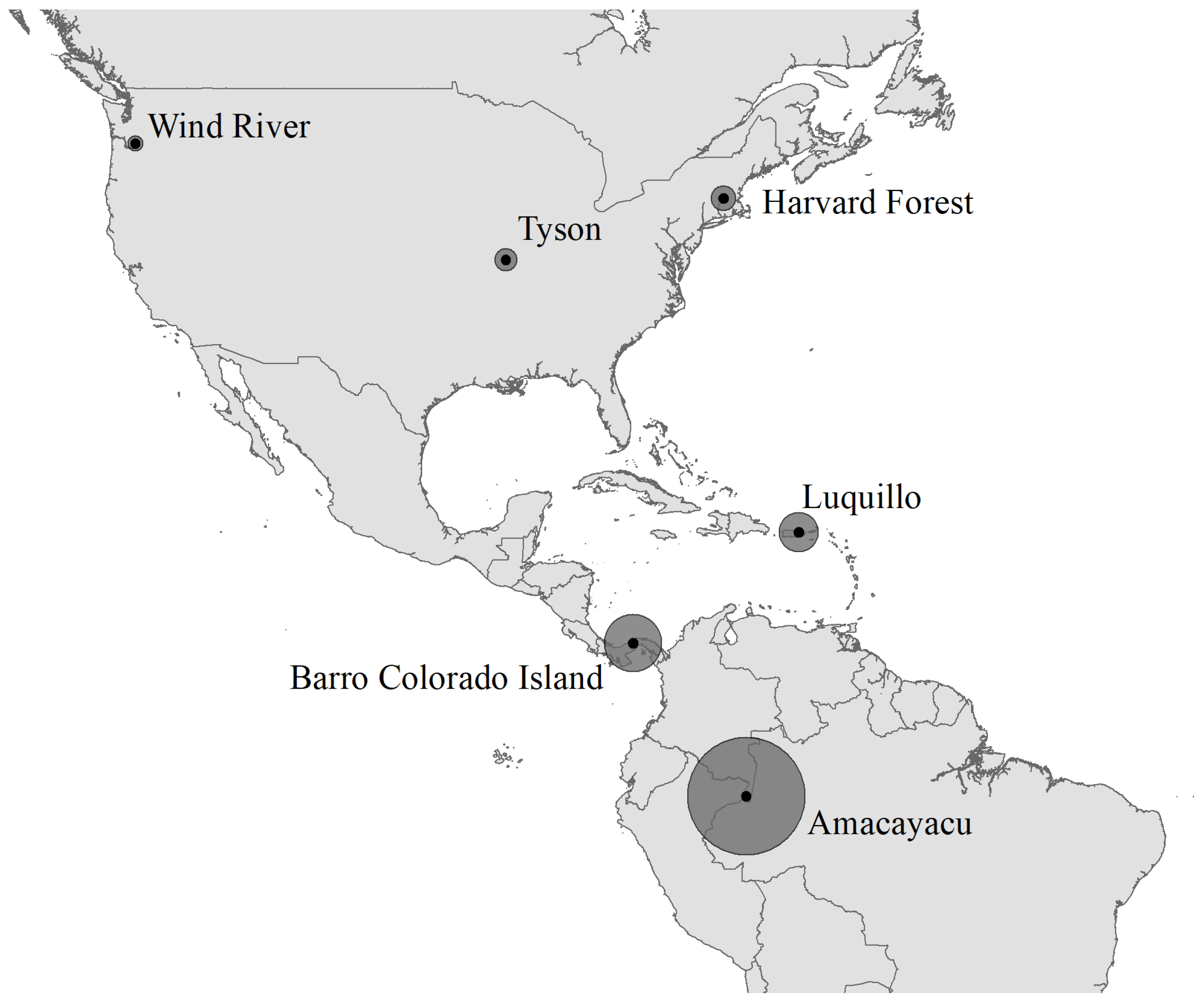
2.1. Forest Dynamics Plots in the Americas

We sought to identify potential foundation species and their relationships to diversity of associated woody plant species in six of the large, permanent Smithsonian ForestGEO (Forest Global Earth Observatory: https://forestgeo.si.edu/) Forest Dynamics Plots. These six plots (three in the north temperate region of the United States and three in the American tropics) span a temperate-to-tropical latitudinal and species-richness gradient in the Western Hemisphere (Figure 1). They are part of the 67-plot global network of ForestGEO research sites that have been established continually since 1980 and re-surveyed at ≈5-year intervals to monitor forest dynamics, effects of climate, and more recently, carbon fluxes and associated microbial and macrobial fauna [24]. Importantly, data among these plots are directly comparable because tree-census protocols are common to all ForestGEO plots. All individuals of woody plant species (canopy and understory trees, understory shrubs, woody vines and lianas) ≥1 cm in diameter at breast height (“DBH;” 1.3 m) are tagged, identified, measured, and mapped at ≈5-year intervals using standardized protocols [25].
The three temperate plots are all in the USA, and include Wind River in southwest Washington State, Harvard Forest in Massachusetts, and Tyson Research Center in Missouri (Figure 1). The 25.6-ha Wind River plot (“WR”; 45.82 °N) is located in a late-seral Pseudotsuga menziesii/Tsuga heterophylla forest of the T.T. Munger Research Natural Area of the Gifford Pinchot National Forest. WR is at ≈365 m a.s.l. and receives ≈2500 mm of precipitation yr−1, much of which falls as snow, leading to a 2–3 month summer dry season [26]. Half of the aboveground biomass at WFDP is concentrated in trees ≥ 93 cm DBH [27]. Regeneration of most species occurs preferentially in gaps created by windthrow [28], and large-diameter trees strongly inhibit recruitment [29].
The 35-ha Harvard Forest plot (“HF”; 42.54 °N) is a mix of deciduous and evergreen trees located at the Harvard Forest Long Term Ecological Research Site within the Worcester/Monadnock Plateau ecoregion [30] of transition hardwood/Pinus strobus/Tsuga canadensis forests [31]. HF is at ≈350 m a.s.l. and receives ≈1150 mm of precipitation (as rain and snow) yr−1 [32]. The HF plot is part of the Prospect Hill tract at Harvard Forest and has a mixed history of land-use and disturbance that includes selective logging and partial clearing for pasturage through the late 1800s, various outbreaks of nonnative pathogens and insects in the 1900s, and periodic hurricanes (in 1815 and 1938) and ice storms (most recently in 2008) [33,34,35].
The 20-ha Tyson plot (“TY”; 38.52 °N) is a late-successional temperate deciduous oak-hickory forest located at Washington University in St. Louis’ Tyson Research Center on the northeast edge of the Ozark plateau. TY is at ≈200 m a.s.l. (elevational range 172–233 m a.s.l.), receives ≈ 1000 mm precipitation (as rain and snow) yr−1, and contains strong edaphic and topographic gradients typical of the Missouri Ozarks [36,37]. Disturbance history at TY includes moderate grazing and selective logging in the early 1900s [38] and extreme droughts in 1988 and 2012. TY has remained relatively undisturbed by humans for ≈80 years [38].
The three tropical plots are in the Caribbean, Central America, and South America. The 16-ha Luquillo plot (“LFDP”: 18.20 °N) is located within the University of Puerto Rico’s El Verde Research Area of the Luquillo Experimental Forest on the Caribbean island of Puerto Rico. This wet tropical forest (≈3500 mm rainfall yr−1) includes a mix of well-conserved and secondary stands (logged and used for subsistence agriculture approximately a century ago) located at ≈380 m a.s.l. [39]. Hurricanes strike the region on average ≈ every 50 years. The most recent large hurricanes (Category 2 or higher) that affected the plot before the census data analyzed here were Hurricanes Hugo (1989) and Georges (1998) [40]. These caused defoliation and branch breakage but relatively little damage to stems, resulting in widespread recruitment of shrubs and sapling trees followed by subsequent thinning as the canopy re-establishes [41].
The 50-ha plot on Barro Colorado island, Panama (“BCI”; 9.15 °N) is on a hilltop that became an island when the Panama Canal was filled and Gatun Lake was created in 1914; the associated Barro Colorado Nature Monument has been managed since 1923 by the Smithsonian Institution. BCI is at ≈140 m a.s.l. and receives ≈2500 mm rainfall yr−1; five–six months of the year make up a pronounced dry season that receives little rain [42,43]. Hurricanes have never been recorded at BCI, and gaps created by single-to-multiple treefalls are the primary type of disturbance observed there [44]. At scales from individual gaps to the entire BCI plot, species diversity is more strongly controlled by recruitment limitation than gap dynamics [44].
The 25-ha Amacayacu plot (“AM”: 3.8 °S) is located within the Amacayacu National Natural Park in Colombia, near the joint border of Colombia, Peru, and Brazil. AM is at ≈93 m a.s.l. within a wet tropical (≈3200 mm rainfall−1) terra-firme forest in the Colombian Amazon [45]. Although topographic relief at Amacayacu varies only over 20 m, it is more tightly associated with woody plant distributions than soil chemistry alone or in combination with topography [45].

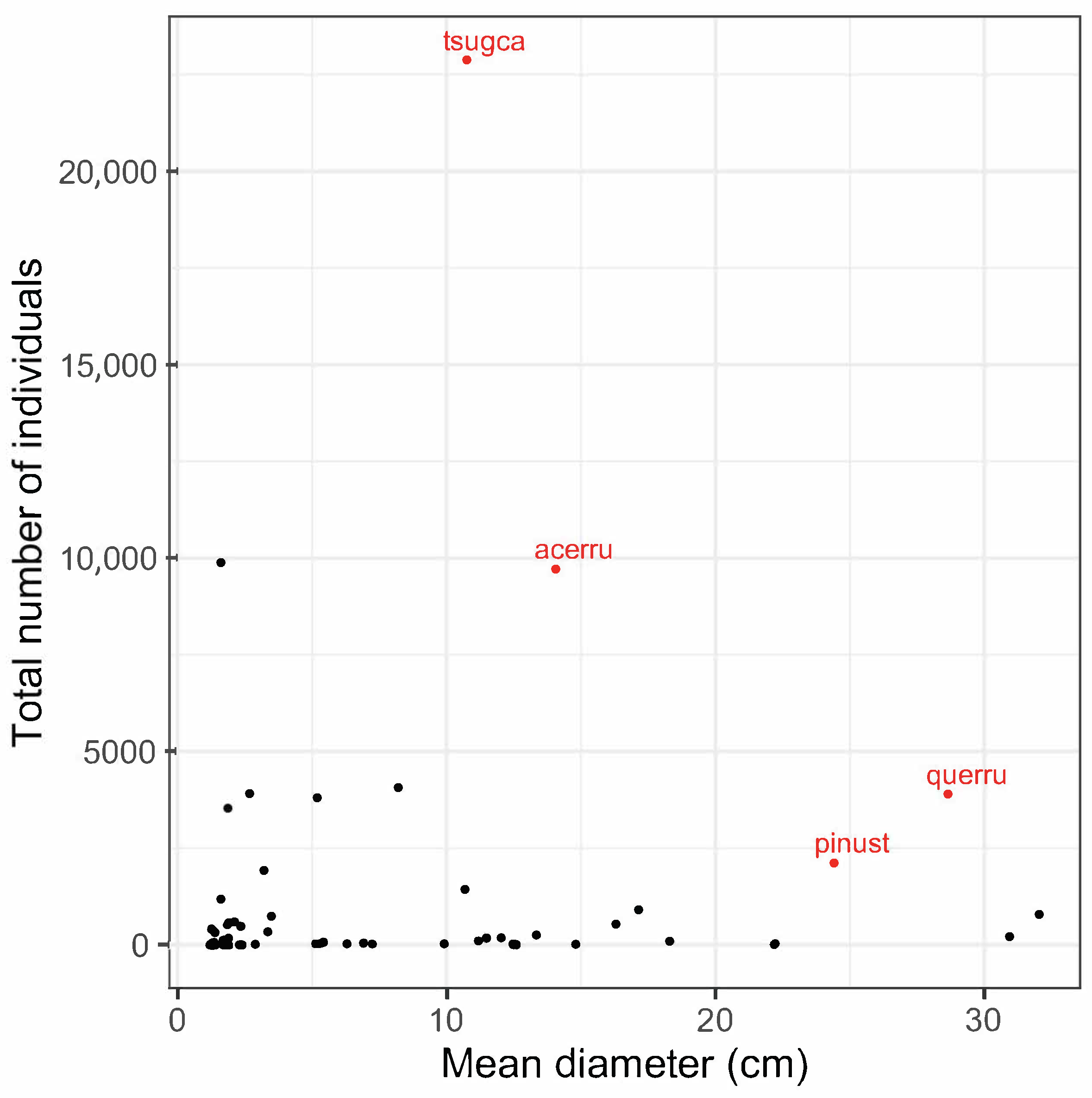
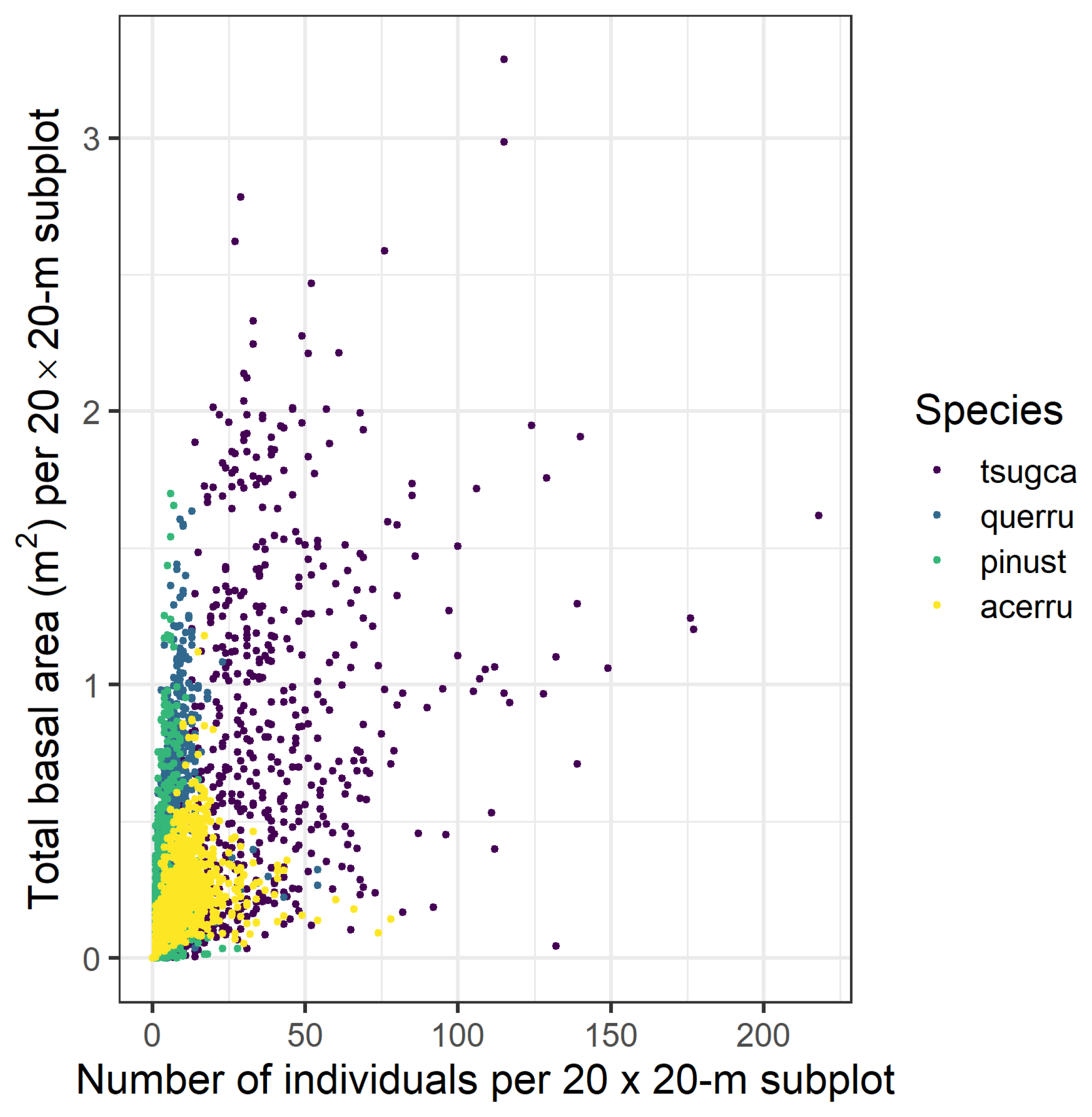
2.2. Identifying Candidate Foundation Species

At HF, four trees numerically dominate the assemblage: Acer rubrum, Quercus rubra, Pinus strobus and Tsuga canadensis. Decades of observational work throughout New England and experimental work at Harvard Forest and elsewhere have consistently supported the hypothesis that T. canadensis is a foundation species whereas the other three are not [16,17]. We started, therefore, by asking whether commonly used graphical assessments of forest structure could distinguish T. canadensis from the other three dominant species. Specifically, we first plotted a basic size-frequency plot for the entire 35-ha Harvard Forest plot; we used DBH of the living woody stems as the measure of tree size and plotted the species-specific mean DBH against the total number of living stems of each of the 51 living woody species in the plot (Figure 2). This size-frequency plot showed a typical “reverse-J” shape [46], but the aforementioned four dominant species were “outliers”, well to the right of the “reverse-J”. To explore the size-frequency relationship of these four species in a more fine-grained way—at the scale at which interactions among individual trees is stronger—we rasterized the plot with a 20-m grid [25]. We then plotted the total basal area of each of the four dominant tree species in each of the 20 × 20-m contiguous subplots within HF (Figure 3). This diameter-abundance plot showed that the foundation species T. canadensis dominated each subplot both numerically and in total basal area, whereas in any given subplot, the other three dominant species either had many individuals or large total basal area, but not both.
We then used these two graphical “fingerprints” to identify dominant species (in terms of abundance and size) in the other five plots (Figure 4 and Figure 5). This analysis identified distinctive species in terms of departure from the “reverse-J” size-frequency distribution at the three temperate plots (Tsuga heterophylla and possibly Pseudotusga menziesii and the subcanopy tree Acer circinatum at WR; three Quercus spp. at TY), and at two of the tropical plots (the canopy tree Dacryodes excelsa and the understory palm Prestoea acuminata at LFDP; and Eschweilera coriacea at Amacayacu) (Figure 4). Other than P. menziesii, A. circinatum, and E coriacea, these species also had basal area-abundance distributions similar to that seen for Tsuga canadensis at HF (Figure 5). For the tropical sites, we also included in subsequent analyses species identified by the site PIs, who established these forest dynamics plots and are co-authors of this paper, as being of known importance for forest dynamics (Table 1). Among these, Oenocarpus mapora at BCI had a basal area-abundance distribution similar to that seen for T. canadensis at HF (Figure 5), but it fell within the “reverse-J” cloud of points in the diameter-abundance distribution (Figure 4). We also included in our analysis several additional species at WR and TY that were identified by the site PIs as ecologically important. These included the canopy species Abies amabilis at WR and three Carya species at TY; and the understory or lower canopy species Taxus brevifolia at WR; and Asimina triloba, Cornus florida, Lindera benzoin, and Frangula caroliniana at TY.

2.3. Metrics of Forest Structure and Species Diversity

For each of the focal species (Table 1), we calculated the total number of stems, the total basal area and the mean basal area at both the plot scale (Table 1) and within cells of the 20-m raster (i.e., each of the contiguous 20 × 20-m subplots within each plot). In each subplot, for the remainder of the woody plant community (i.e., all species other than the focal species), we calculated the total abundance of stems, the total number of species, the Hill-number equivalents of Shannon’s diversity and the inverse Simpson’s indices [47], and the mean Bray-Curtis dissimilarity (of each subplot relative to each of the other subplots in the raster [48]; the latter is a measure of how “modal” or “outlying” each subplot is in its species composition relative to all other grid cells. For the calculation of Bray-Curtis dissimilarity, empty grid cells (i.e., those with no species other than the focal species) were assigned a dummy-value (“empty”) to allow the calculation of all pairwise dissimilarities; this means that all empty cells appear to be maximally different from occupied cells, but maximally similar to each other. For all datasets, we used only the records for the main stem of each species, thus removing any additional stems; this eliminated the problem in spatial analyses of having multiple stems at the same point location. Initial exploration of the data showed that the effect of removing additional stems (primarily of small shrubs) on relative patterns in stem abundance and basal area was negligible for most species across all datasets. The diversity() and vegdist() functions in the R vegan package [49] were used for calculating each diversity metric.

2.4. Codispersion Analysis

Codispersion analysis quantifies the spatial association between two variables measured at individual spatial locations or on a grid [19]. Here, we examined codispersion between the total basal area of each focal species in each subplot of the 20-m raster versus each of the community metrics summarizing the diversity and composition of the other species in same subplot [20]. The spatial association quantified by the codispersion coefficient ranges from −1 to 1, where positive values represent a positive spatial association and negative values represent a negative spatial association. The results are presented as a hemispherical codispersion graph, which shows how the coefficient changes with distance (i.e., spatial lags) and direction (angles around a hemisphere). Thus, differences observed at different spatial lags indicate the scale(s) over which spatial processes are operating within the forest plots, whereas differences in the strength or sign of the correlation in different directions are diagnostic of anisotropic spatial processes [20]. To ensure sufficient sample size when computing codispersion coefficients between measurements made in 20-m grid cells (the size of each subplot), we used spatial lags in 20-m intervals from 20 to one-quarter the size of the minimum dimension of each plot [50]. We calculated codispersion coefficients using code custom-written and compiled in C (to reduce computation time), but with a link to R that allows for easy manipulation of input and output datasets [51].

2.5. Significance Testing with Null Model Analysis

For each dataset, focal species, and community metric combination, we recalculated the codispersion 199 times using the observed focal species total basal area raster and both (1) community metric rasters calculated from the point-pattern of the other species under a random shift around a torus (“toroidal-shift" null model) and (2) a spatially randomized raster of the community metric for the other species in the community (“CSR” null model) [21]. For each null model, the observed codispersion value for each cell was then compared to the distribution of the 199 null values and deemed significant if it fell outside 95 percent of the values (i.e., a two-tailed test). The toroidal-shift null model breaks the spatial association between the focal species and the other species in the community but retains any larger-scale spatial patterns, making this test slightly more conservative because it accounts for spatial patterns caused by the environment. In contrast, the CSR null model breaks the spatial association between the focal species and the other species in the community and simultaneously randomizes any larger-scale spatial patterns caused by environmental patchiness in the plots.

2.6. Data and Code Availability

Each of the ForestGeo plots were established at different times and have been censused every five years. To maximize comparability among datasets, we used data collected within a fifteen year period: the first censuses at Wind River (2010–2011), Harvard Forest (2010–2012), Tyson (2011–2013), and Amacayacu (2008–2009), the third census at Luquillo (2000), and the eighth census at BCI (2015). All datasets are available from the ForestGEO data portal https://ctfs.si.edu/datarequest). R code for all analyses is available on GitHub (https://github.com/buckleyhannah/FS_diversity).

3. Results

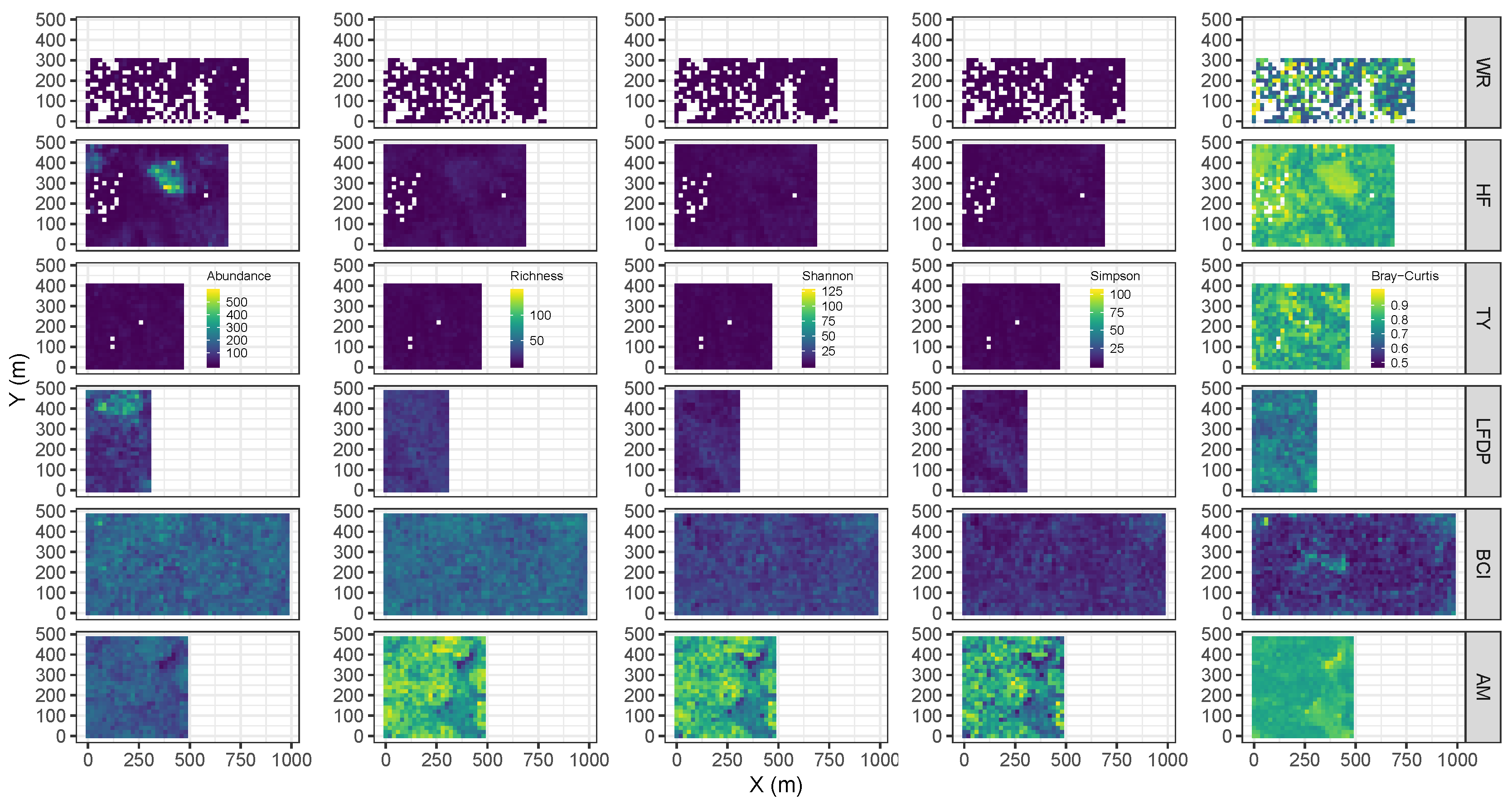
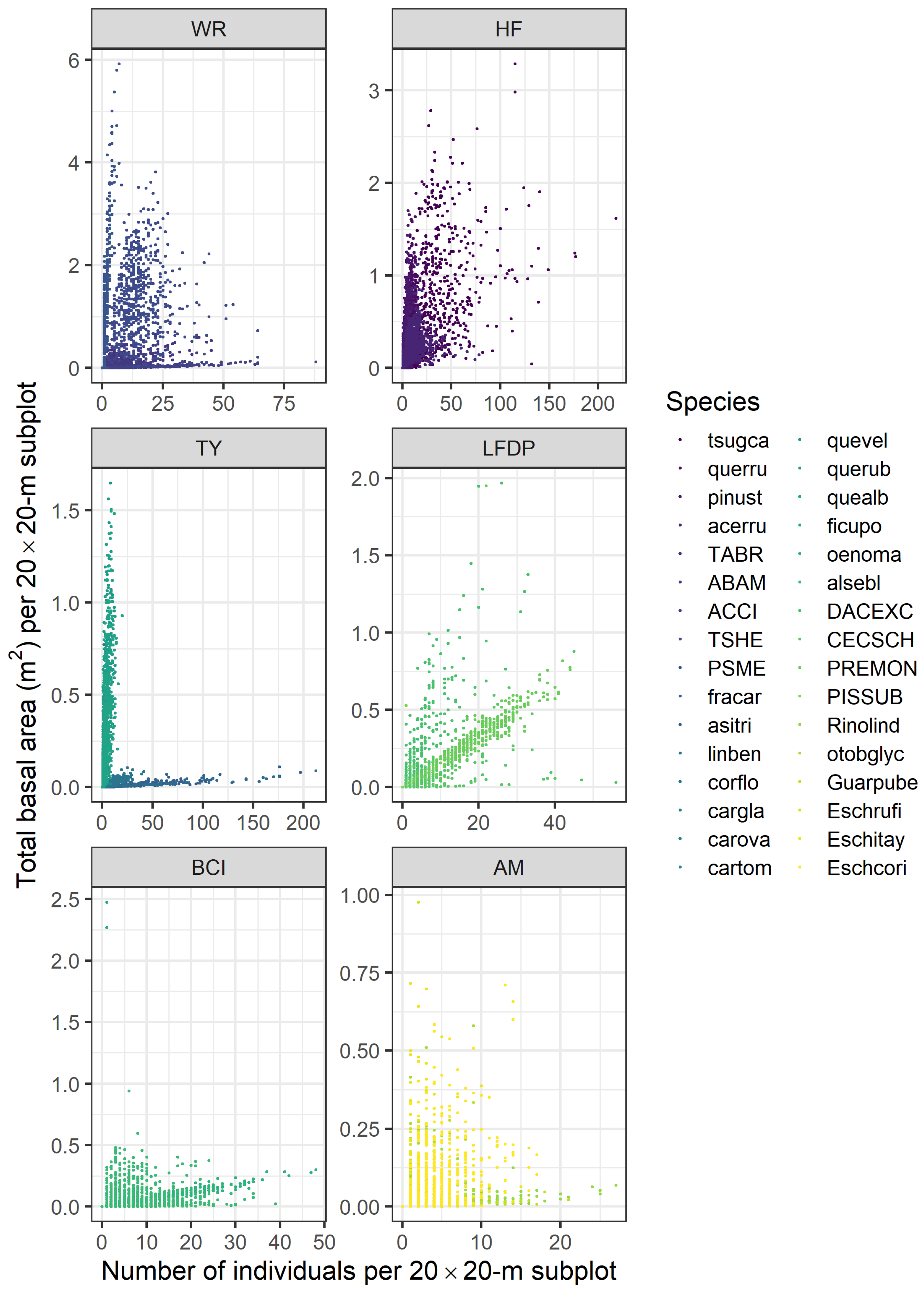
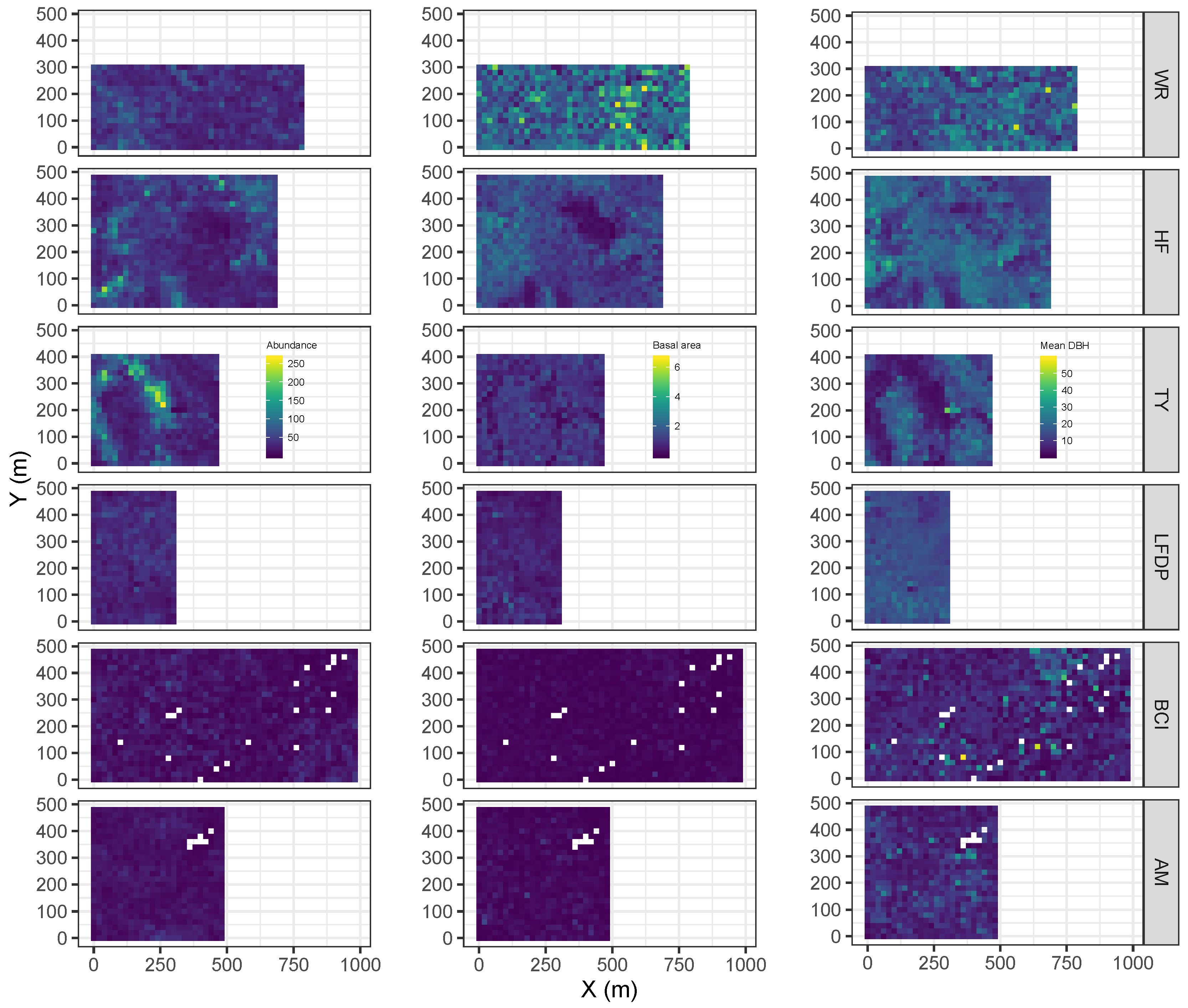
3.1. Forest Structure and Species Diversity

Across the entire plots and within the 20 × 20-m subplots, abundance (number of main stems) of the hypothesized foundation species and other focal species was highest in the three temperate plots (Table 1, Figure 6). The average and total basal area of these same species were highest at Wind River (Tsuga heterophylla) and Harvard Forest (Tsuga canadensis) in the temperate region, at least 2–4-fold greater than the most abundant important species in the tropical plots (Dacryodes excelsa at Luquillo and Alseis blackiana at BCI) (Table 1, Figure 6). Note that focal species were absent in some of 20 × 20-m subplots at both BCI and AM (white cells in the bottom two rows of Figure 6). In contrast, abundance, richness, Shannon diversity and Simpson’s diversity of associated species were substantially higher in the three tropical plots than in any of the temperate plots (Figure 7). Average subplot-wise Bray-Curtis dissimilarity of associated species was higher in the three temperate plots and at Amacayacu than at Luquillo or BCI (Figure 7). Note that only focal species were present in many of the 20 × 20-m subplots at WR and in a handful of 20 × 20-m subplots at HF and TY (white cells in Figure 7).

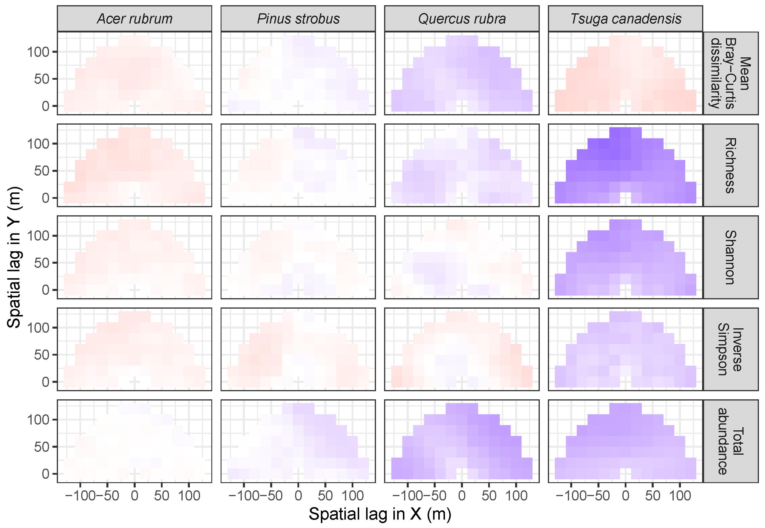
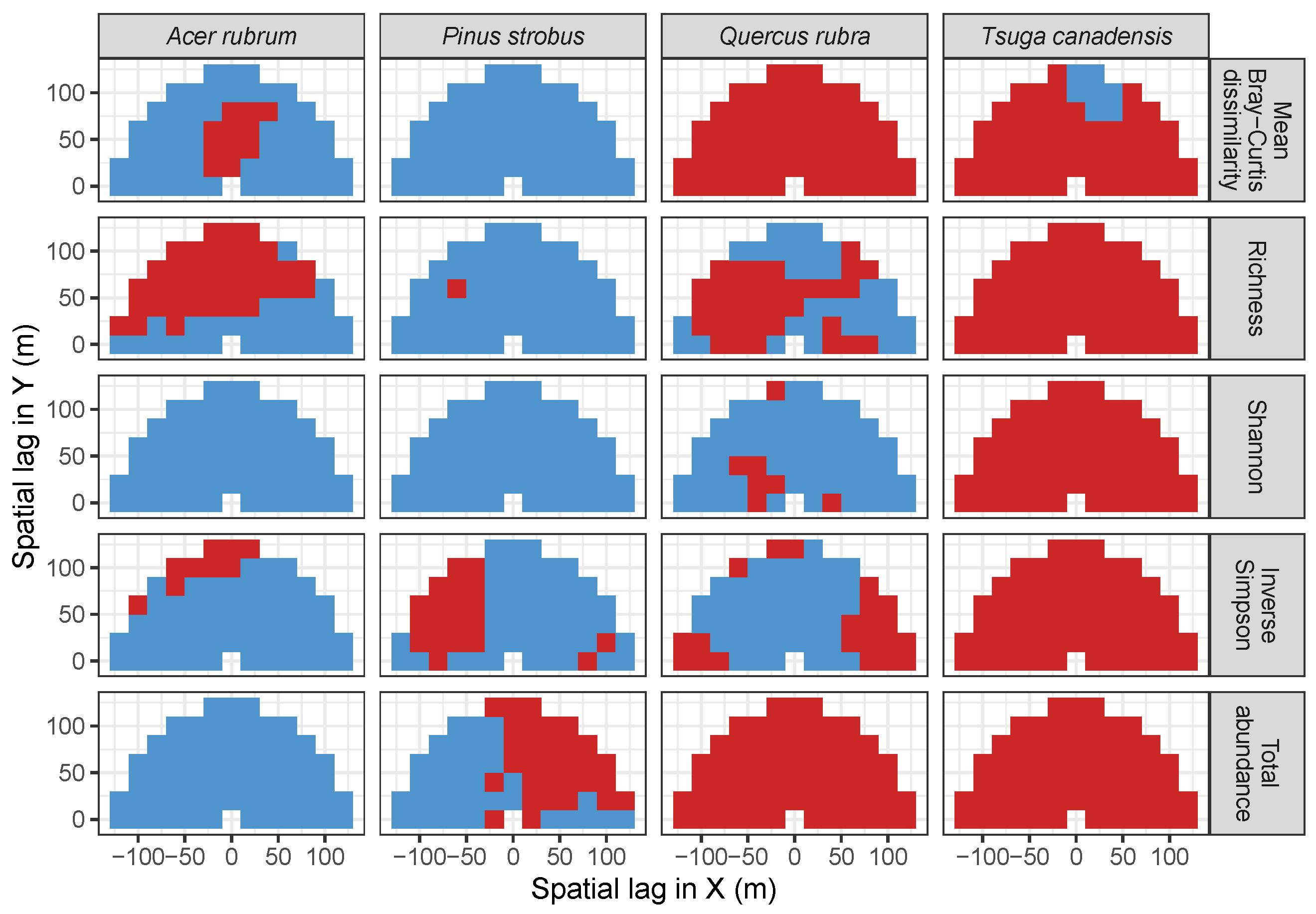
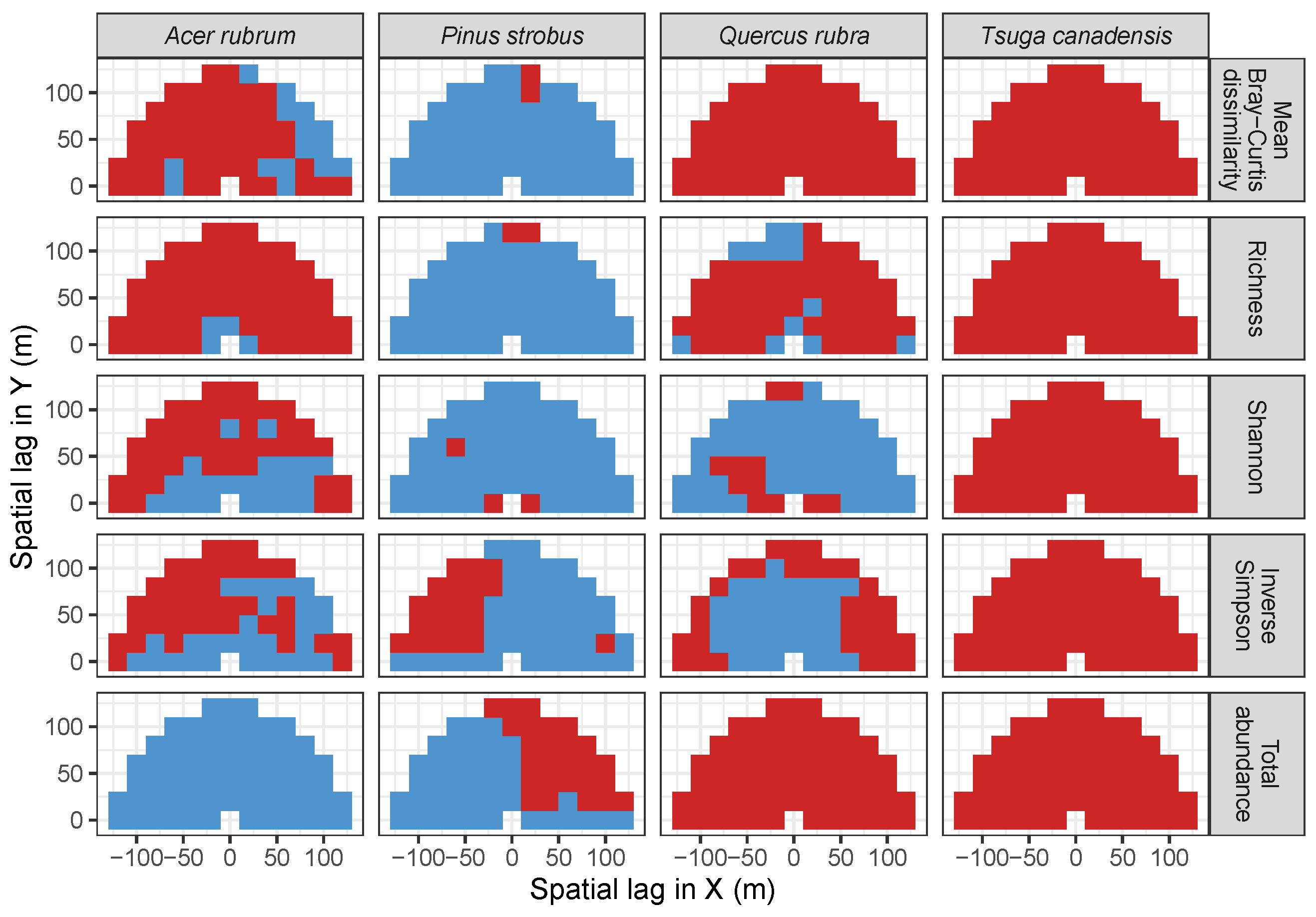
3.2. Codispersion Between Focal Species and Associated-species Diversity at Harvard Forest

As with our initial screen for candidate foundation species, in which we used a graphical “fingerprint” observed for Tsuga canadensis at HF to screen for important species at other sites (Figure 2, Figure 3, Figure 4 and Figure 5), we first examined the codispersion statistics and graphs illustrating spatial associations between metrics of woody plant diversity and total basal area of Tsuga canadensis relative to the other three dominant tree species at HF within 20 × 20-m subplots.
At all spatial lags (computed from 20–125 m) and directions, the strongest and most consistently significant measures of codispersion between total basal area and metrics of associated-species diversity at Harvard Forest were observed for the foundation species, T. canadensis (Figure 8, Table A1). Total basal area of T. canadensis was negatively spatially associated at all spatial lags and directions with the total abundance, species richness, Shannon diversity, and inverse Simpson’s diversity of associated-woody species, but was positively spatially associated at all spatial lags and directions with average Bray-Curtis dissimilarity (Figure 8, Table A1). All of these codispersion coefficients—at virtually all spatial lags and directions—were significant relative to those generated with the more conservative toroidal-shift null models (Figure 9). The few codispersion coefficients that were not significant when tested with the more conservative toroidal-shift null model were significant when tested with the CSR null model (Figure 10). In contrast, codispersion between total basal area of the other three focal species at HF and all metrics of associated-species diversity were weaker and inconsistently significant (Figure 8, Figure 9 and Figure 10, Table A1). Only the consistently positive codispersion between Q. rubra and either abundance of associated woody species or Bray-Curtis dissimilarity were always significant relative to null expectation (Figure 9 and Figure 10). Overall, the absolute value of the mean or median codispersion between total basal area of T. canadensis and metrics of associated-species diversity ranged from 2–10-times greater than the mean or median codispersion between the total basal area of any of the other three dominant tree species and measures of associated-species diversity (Table A1).

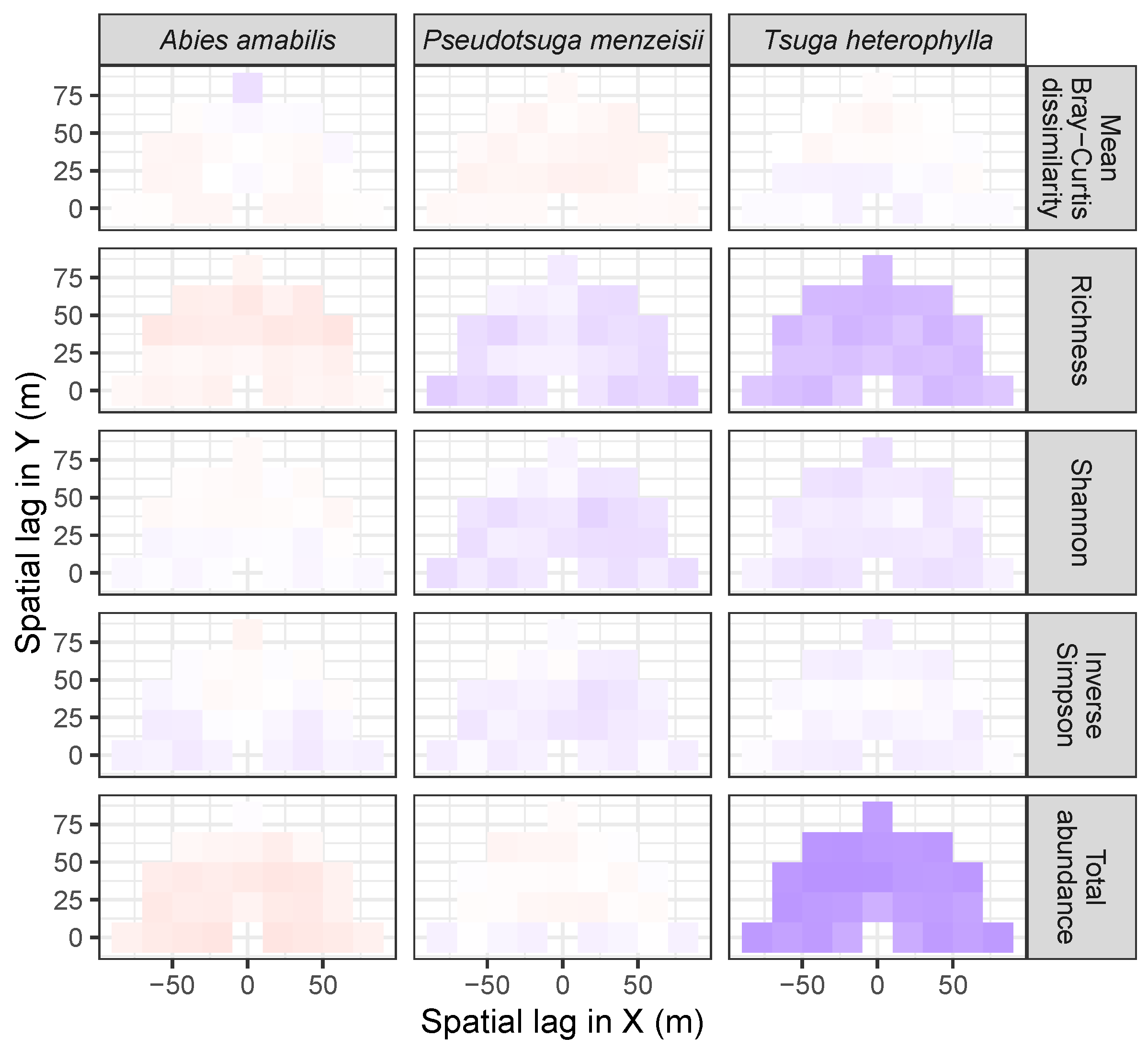
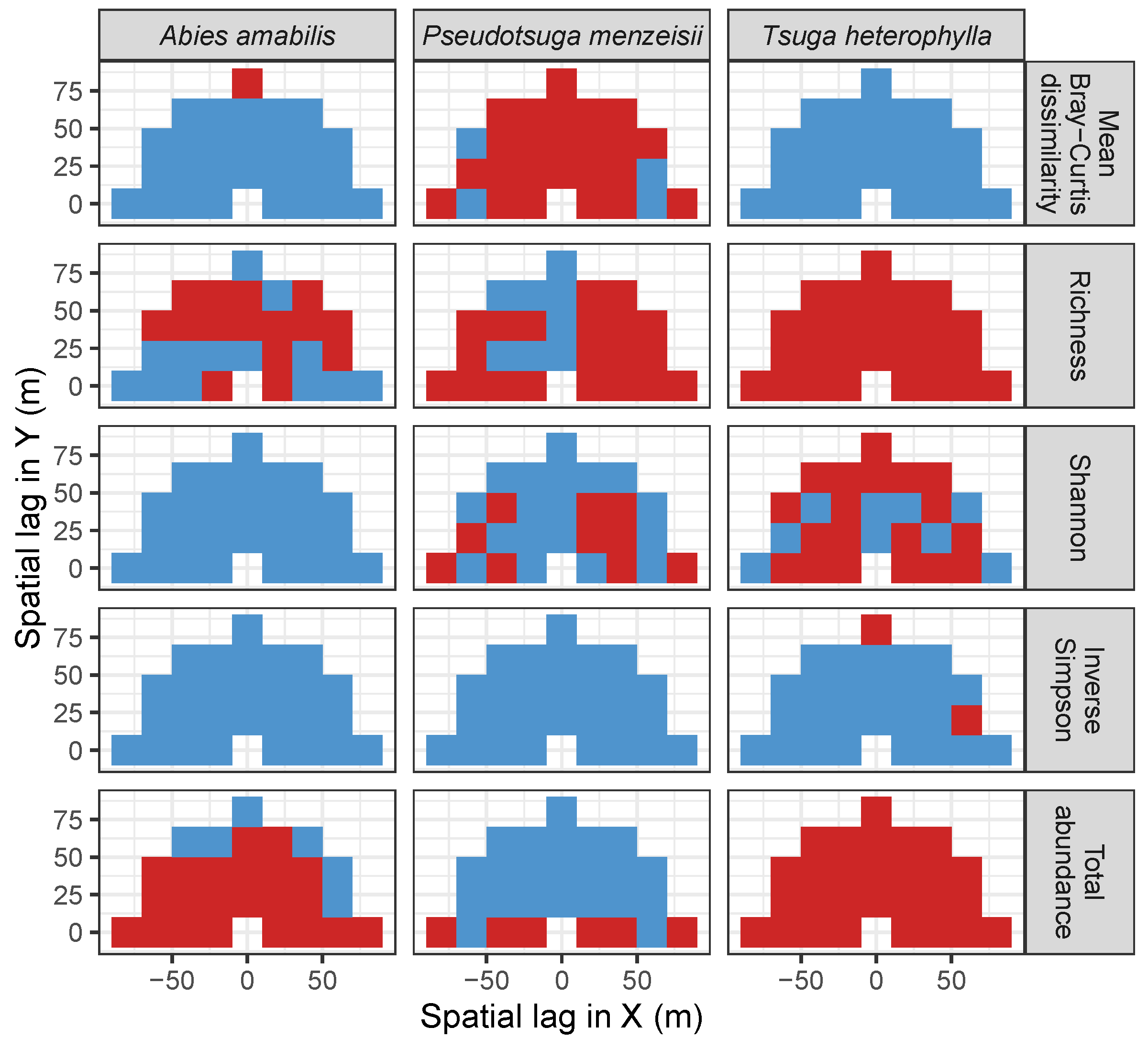
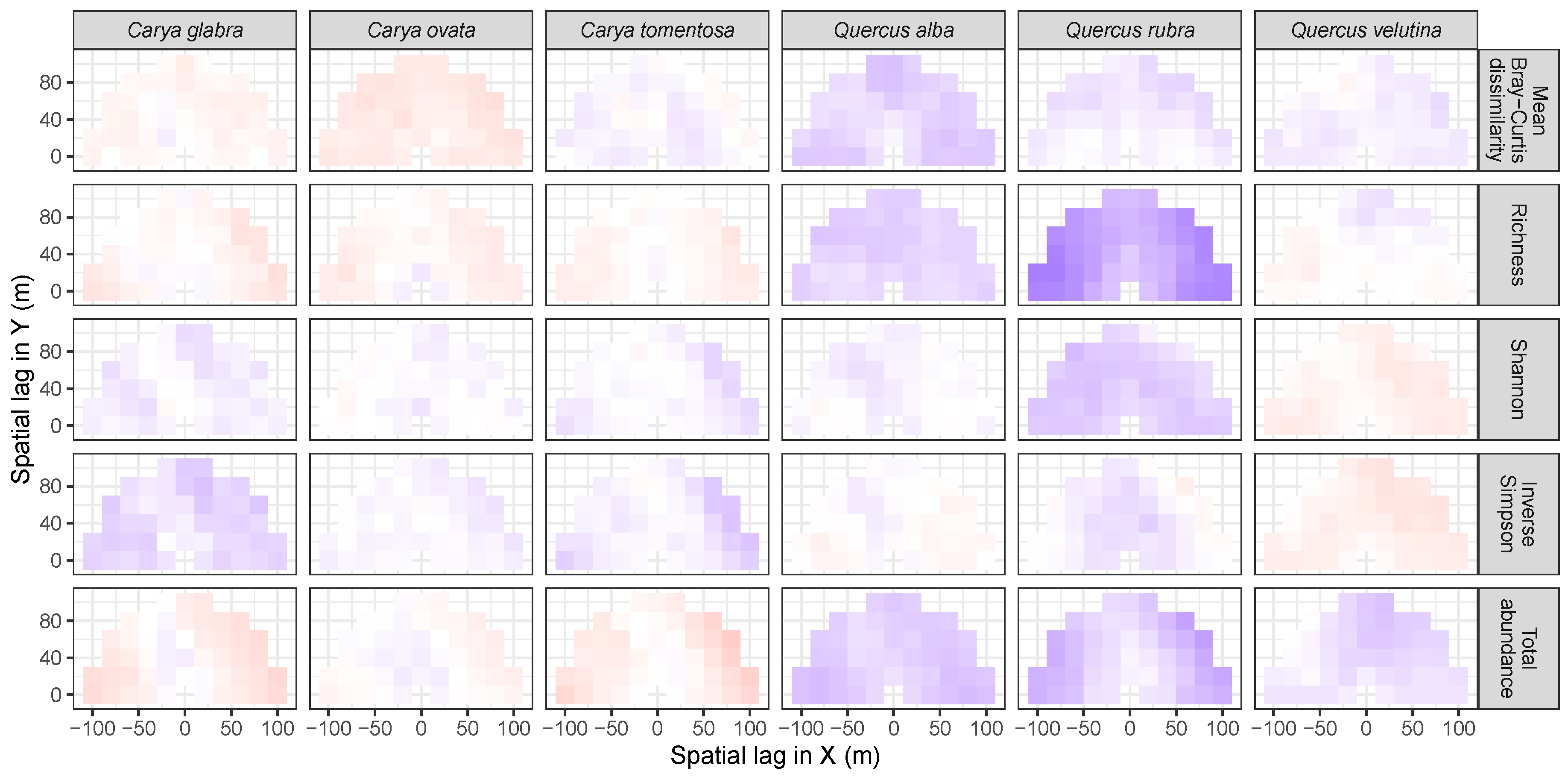
3.3. Codispersion Between Focal Tree Species and Associated-Species Diversity at the Other Five Sites

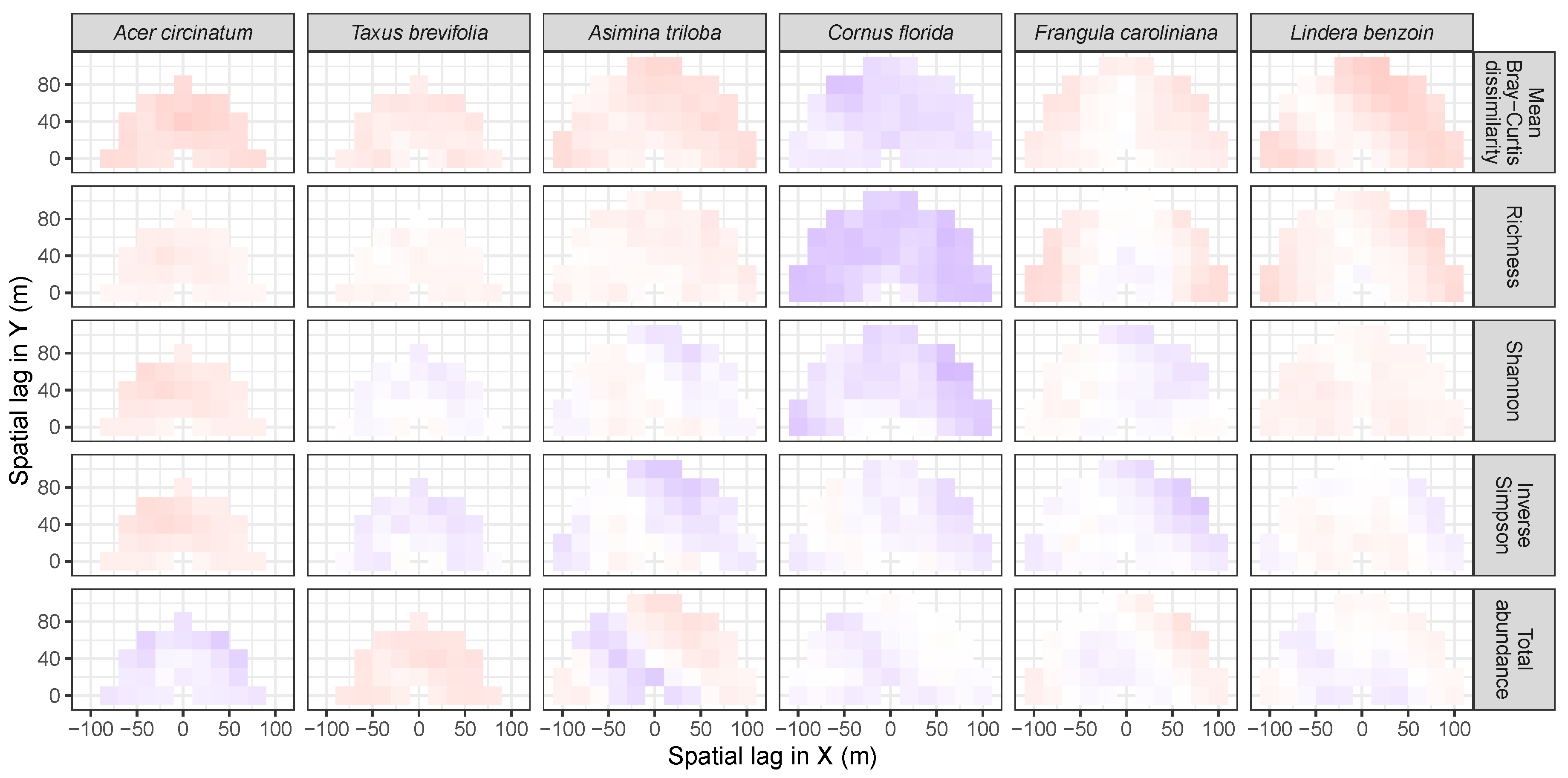
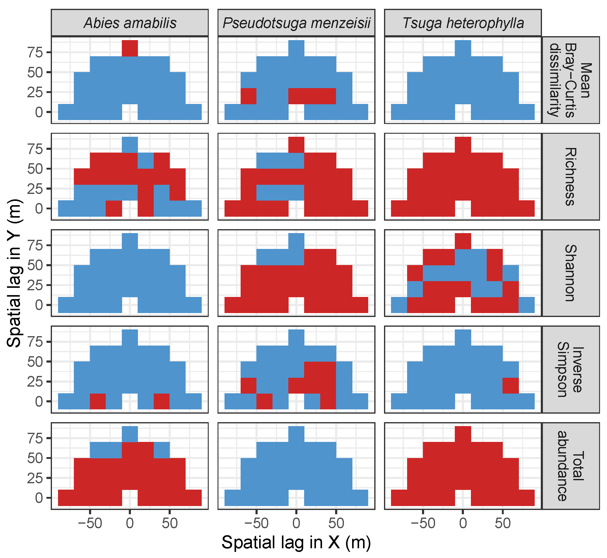
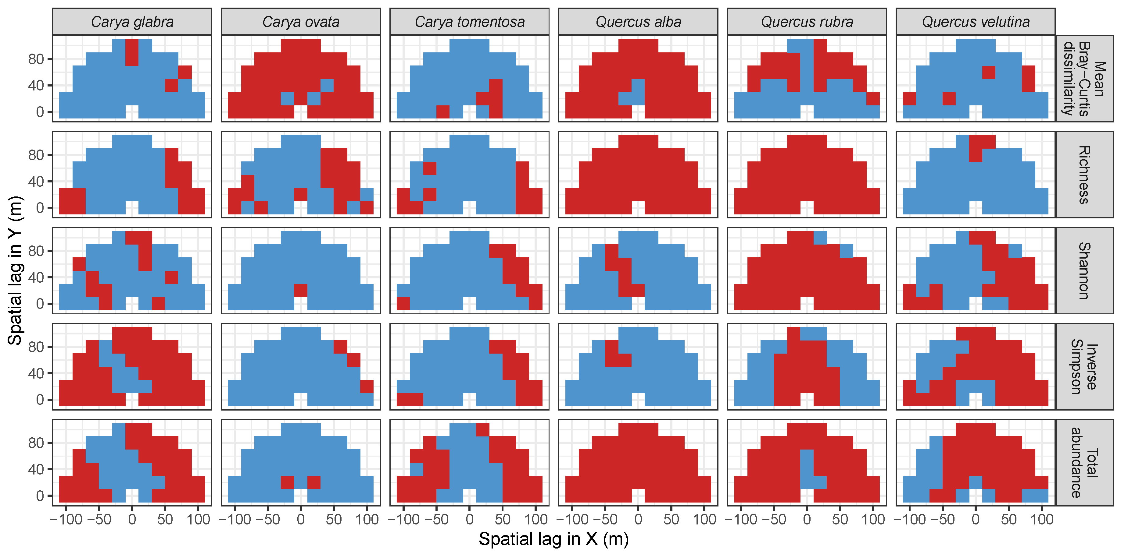
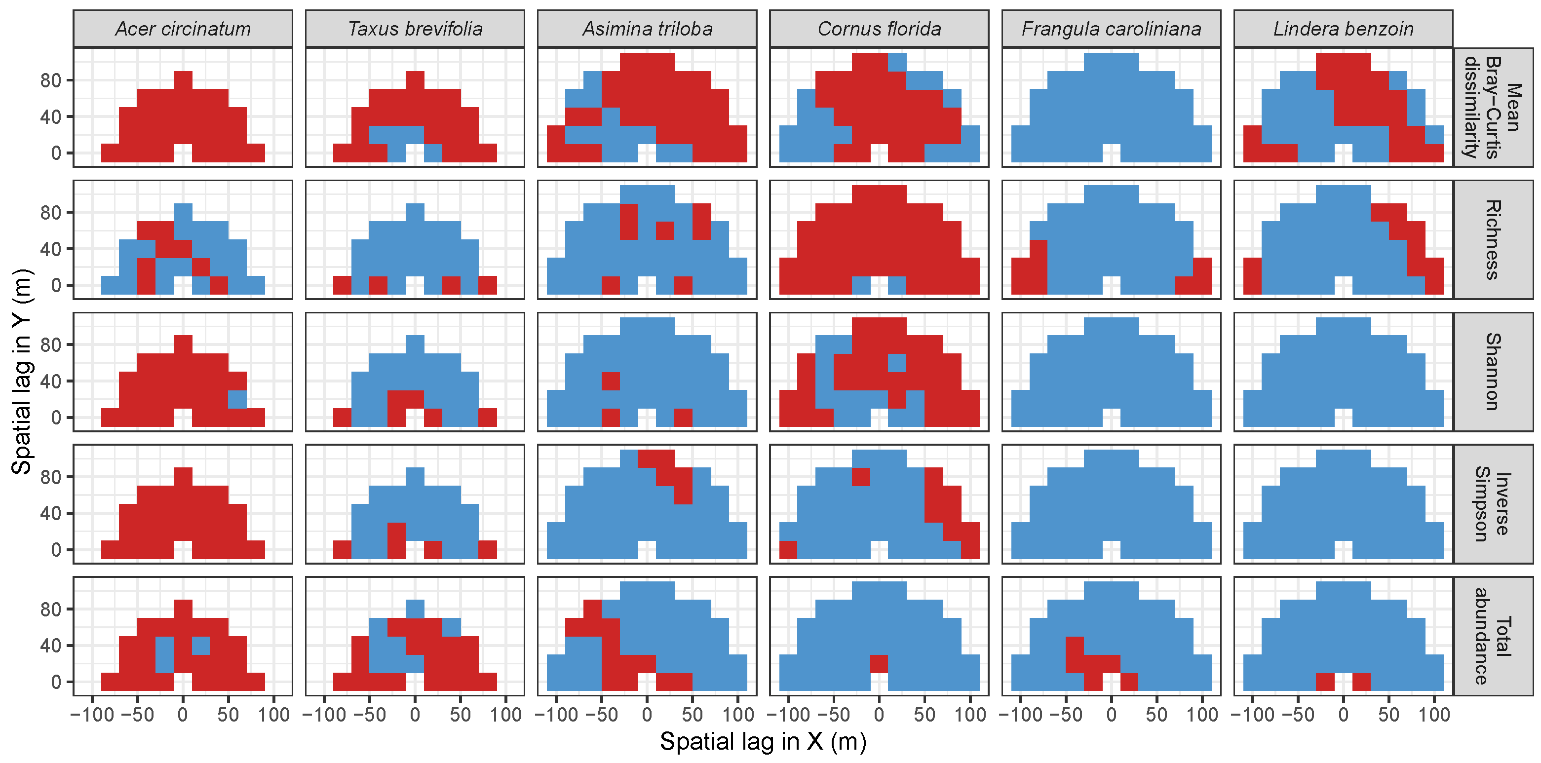
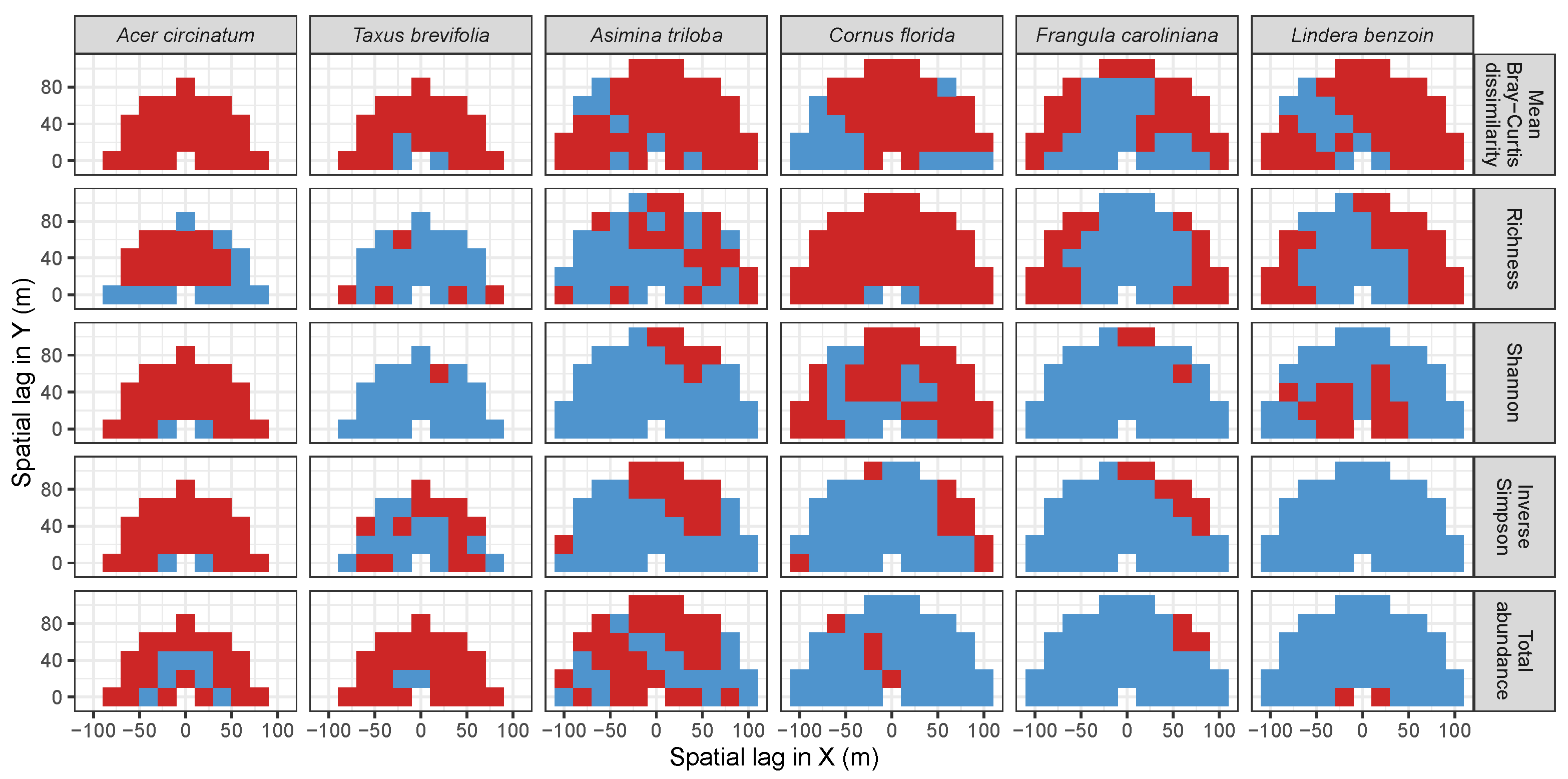
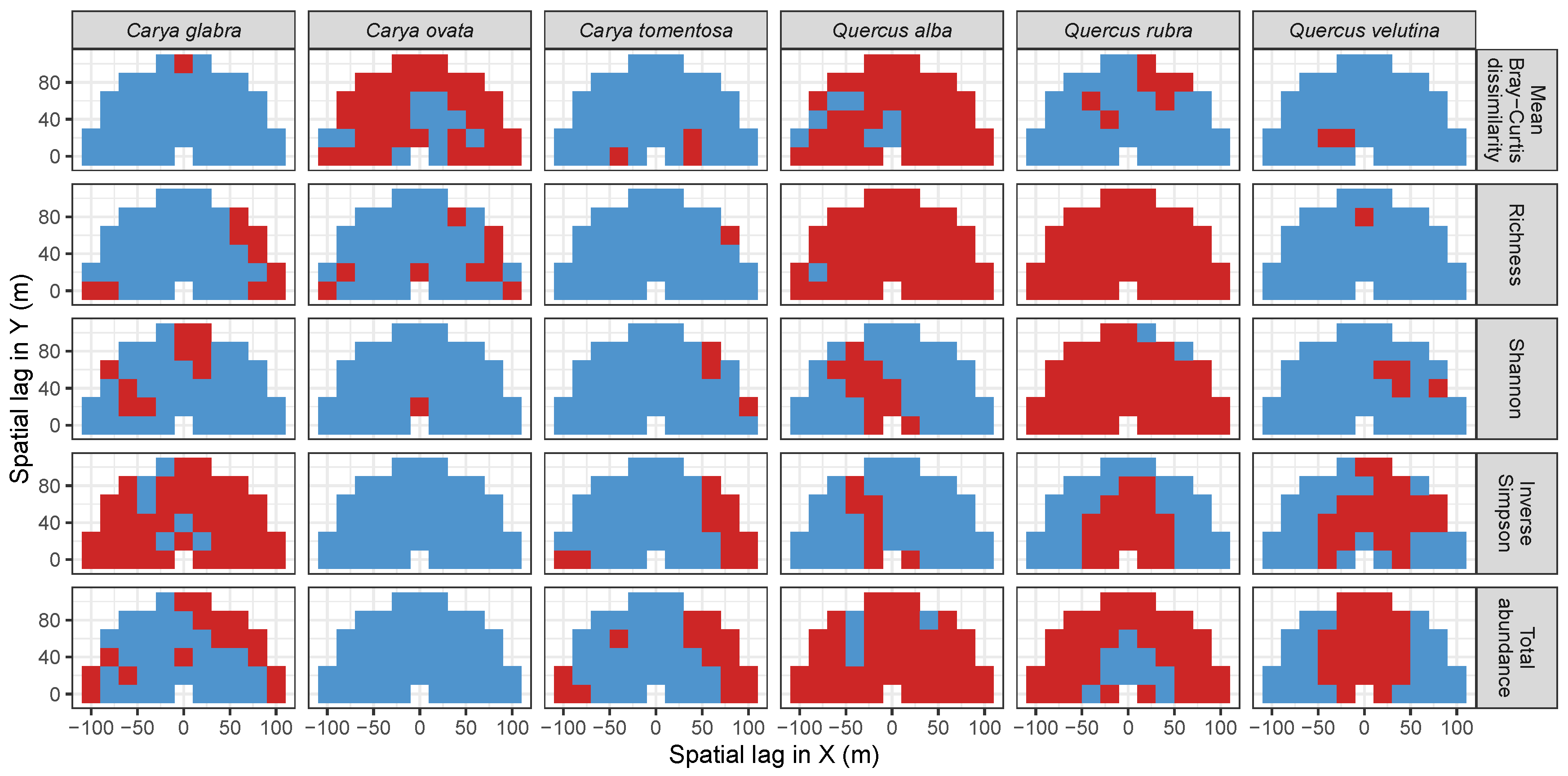
3.3.1. Trees at temperate sites

Observed patterns of codispersion between total basal area of focal species and metrics of associated-species diversity at WR and TY were qualitatively similar to those observed for the non-foundation species at HF. At WR, codispersion between total basal area of Tsuga heterophylla and all measures of diversity was consistently negative (Figure 11) but only significant at all lags and directions for abundance and richness of associated species (Figure A1). Values of codispersion at WR between T. heterophylla and associated-species diversity were much lower than those observed for T. canadensis but similar to those observed for Q. rubra at HF (Table A1). Codispersion between total basal area of Pseudotsuga menziesii and Bray-Curtis similarity was positive, and was significant for about two-thirds of the lags and directions when assessed with the toroidal-shift null model (Figure 12) but not the CSR null model (Figure A1).
At TY, codispersion between associated-species abundance and richness and basal area of two of the oaks—Quercus alba and Quercus rubra—was negative and consistently significant (Figure 13 and Figure 14 and Figure A2). Codispersion between Shannon diversity of associated-species and basal area of Q. rubra was also consistently and significantly negative (Figure 13 and Figure 14 and Figure A2). Codispersion between Bray-Curtis dissimilarity and basal area of Q. alba and Carya ovata were significantly positive and negative, respectively (Figure 13 and Figure 14 and Figure A2). As at WR, the range of observed, significant, codispersion values measured at TY paralleled those measured for Q. rubra at HF (Table A1). A notable exception were the values of codispersion between basal area of Q. rubra at TY and associated-species richness, which were nearly identical to that observed for T. canadensis at HF (Table A1).

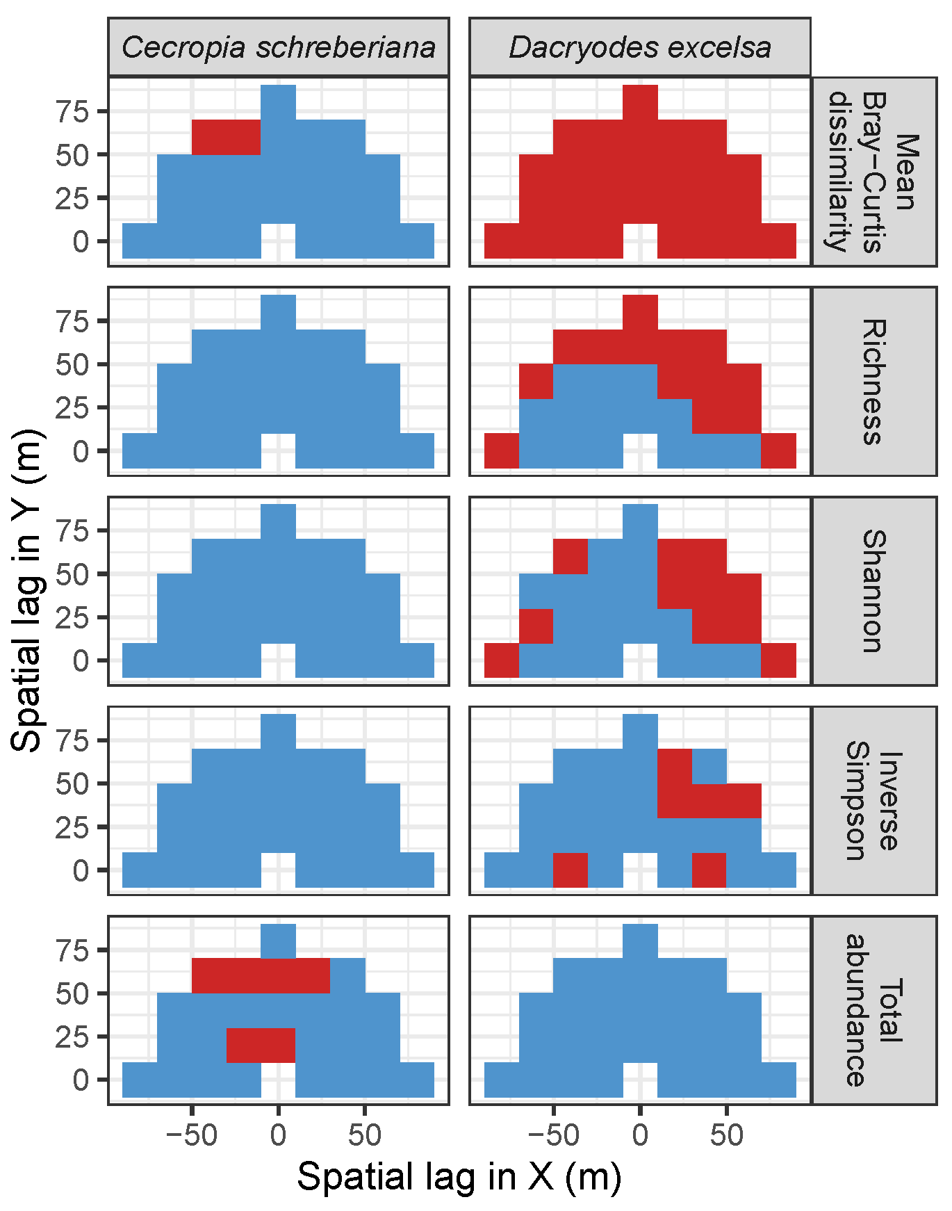
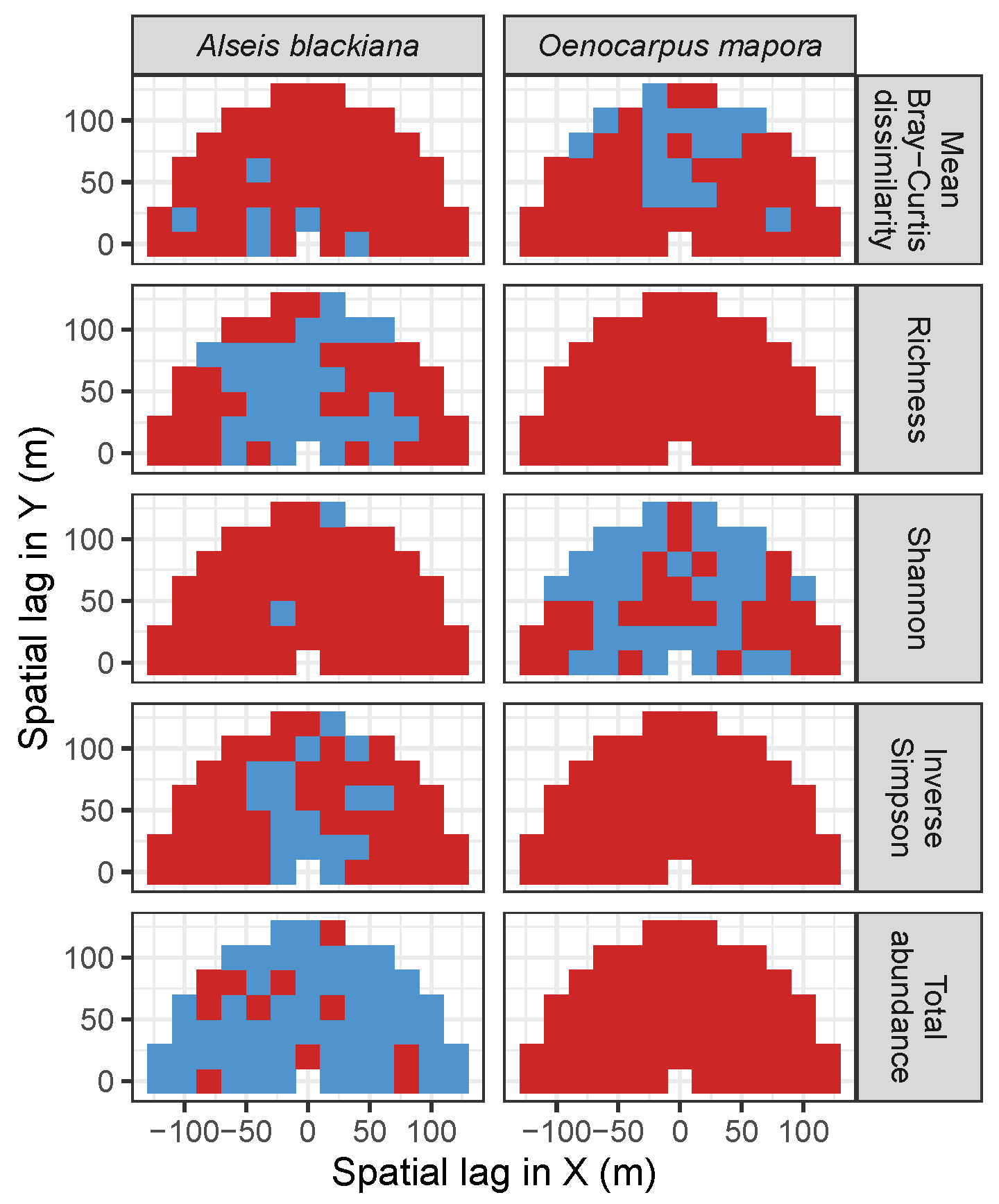
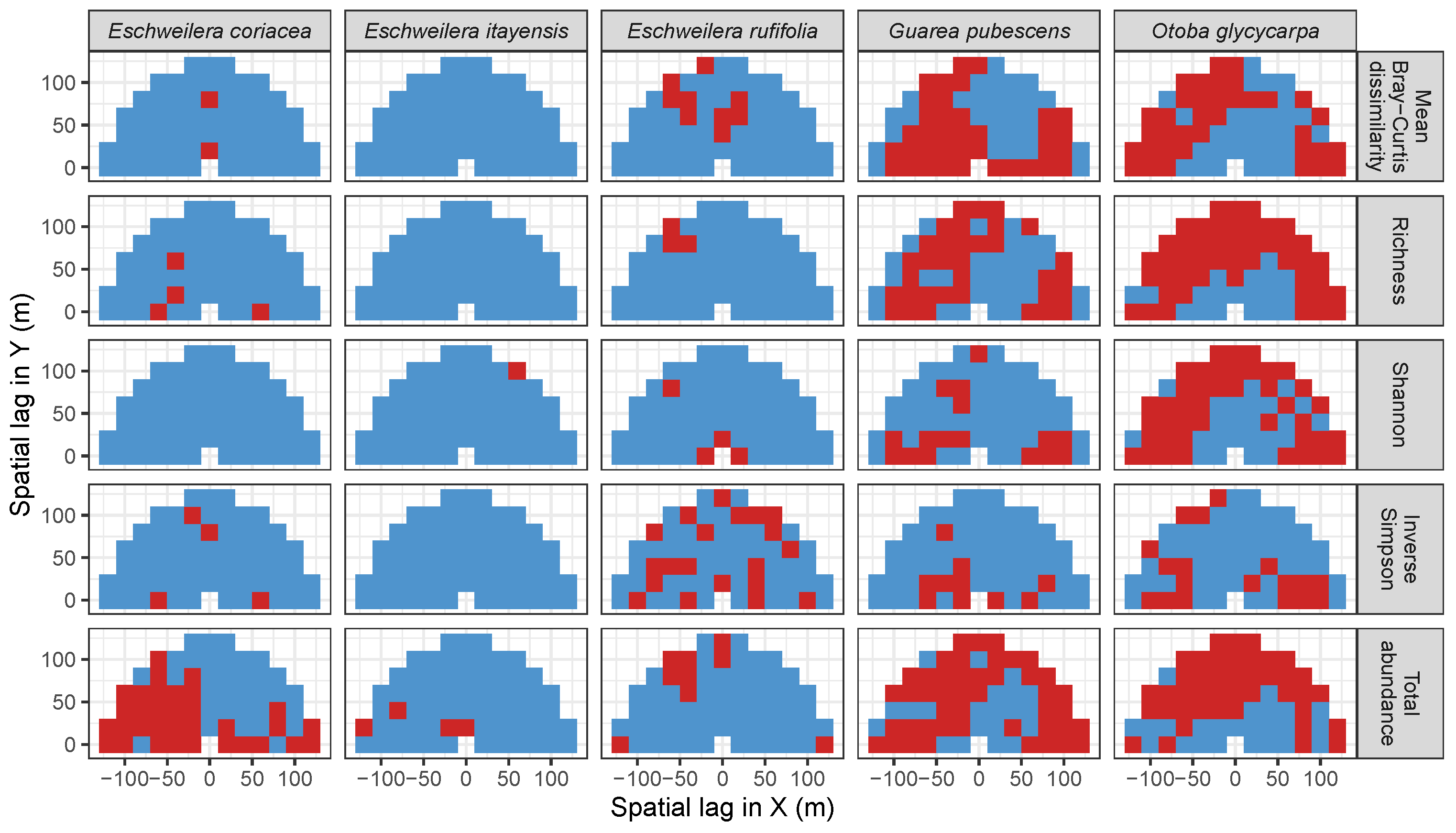
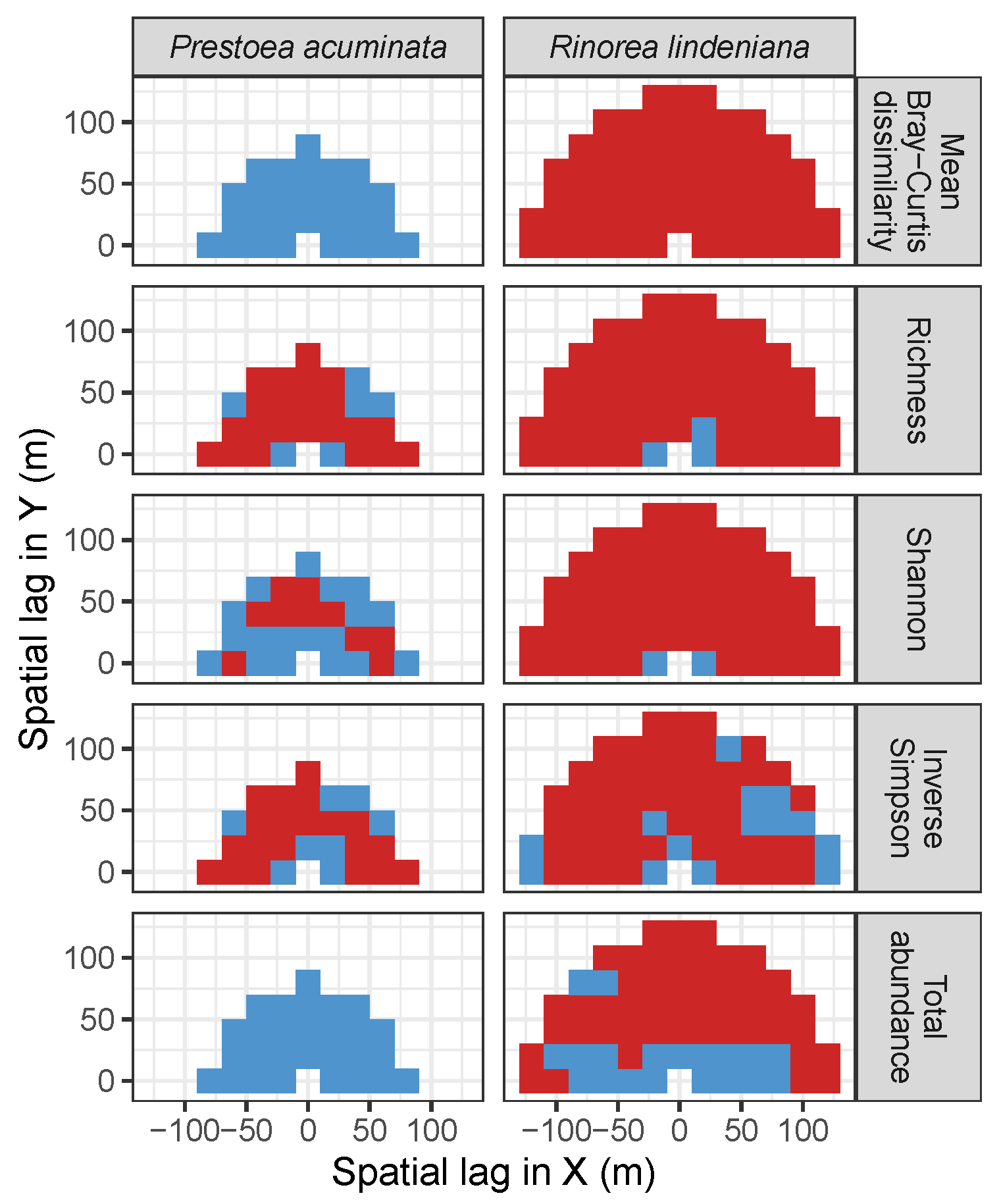
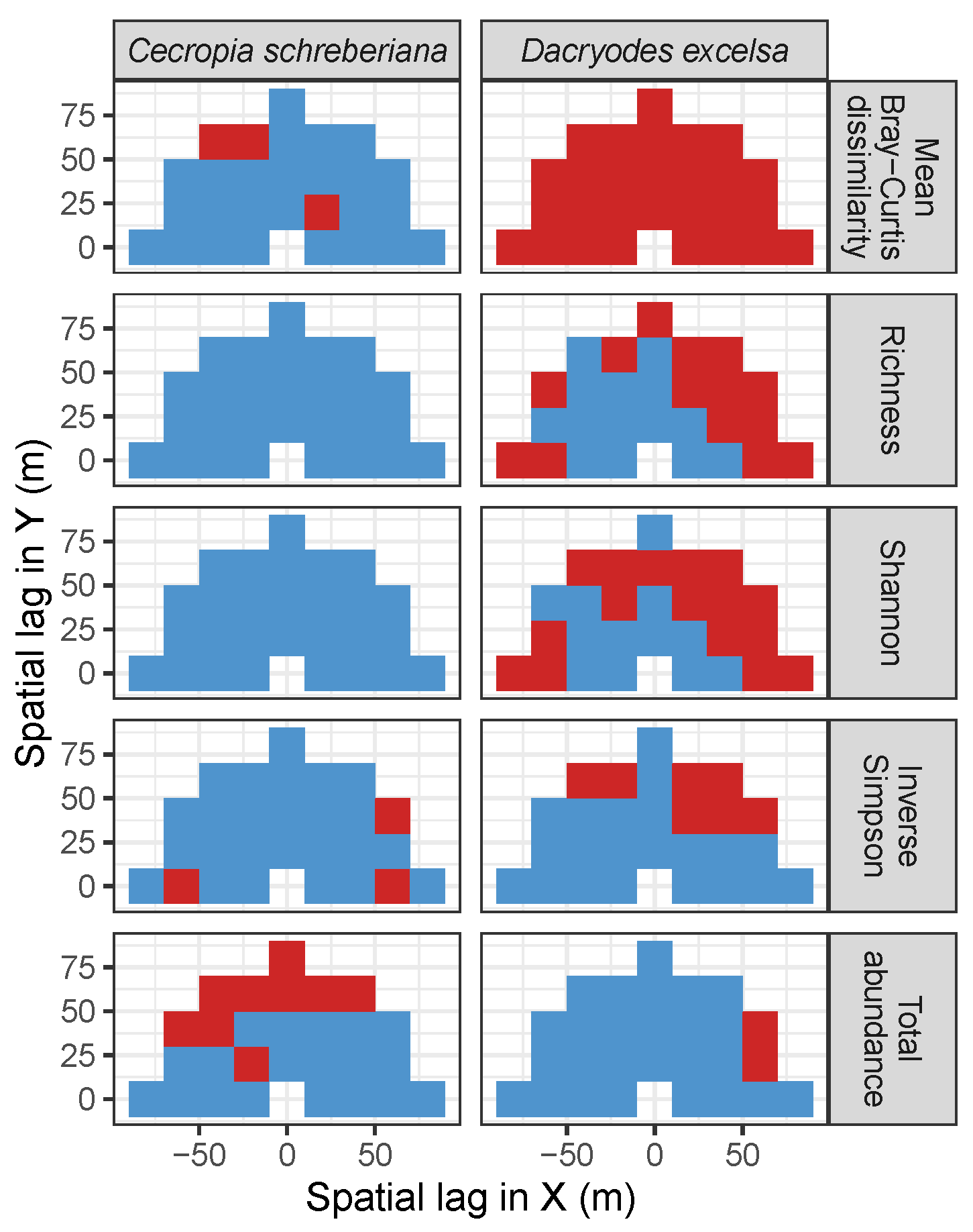
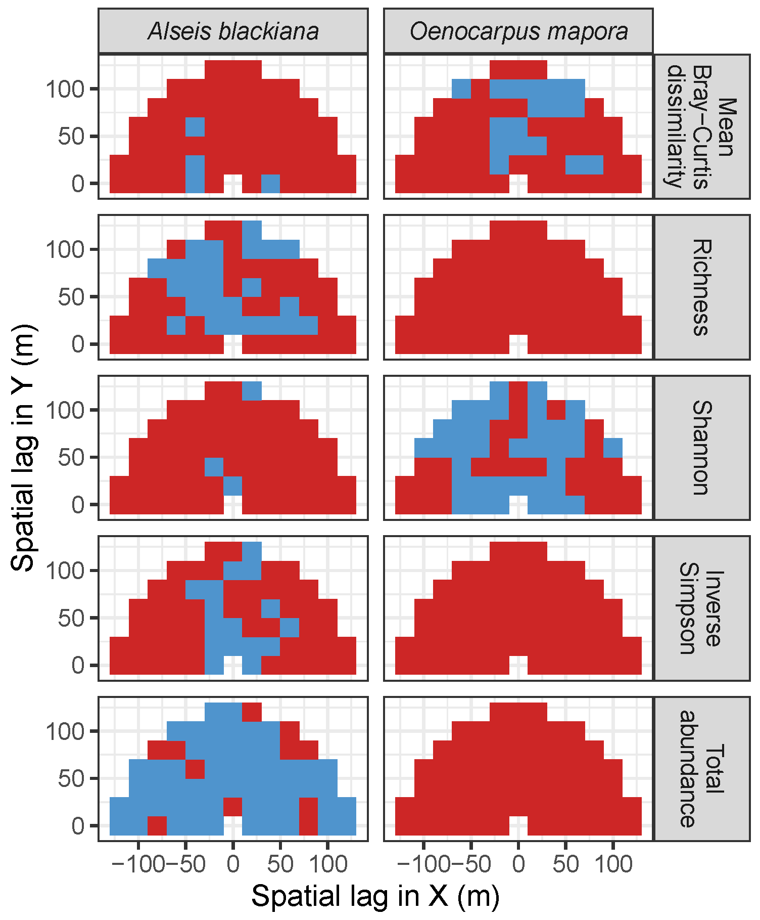
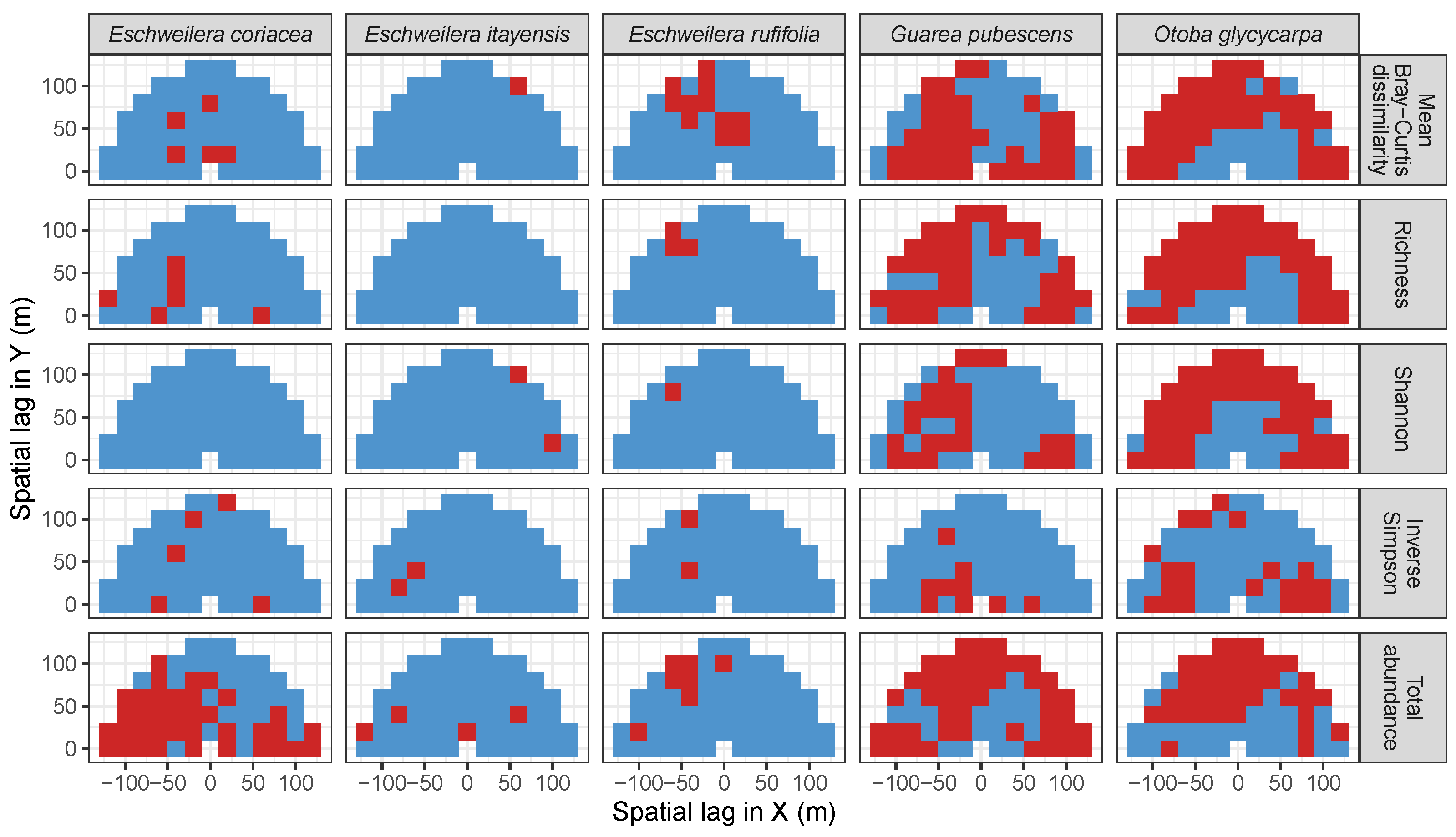
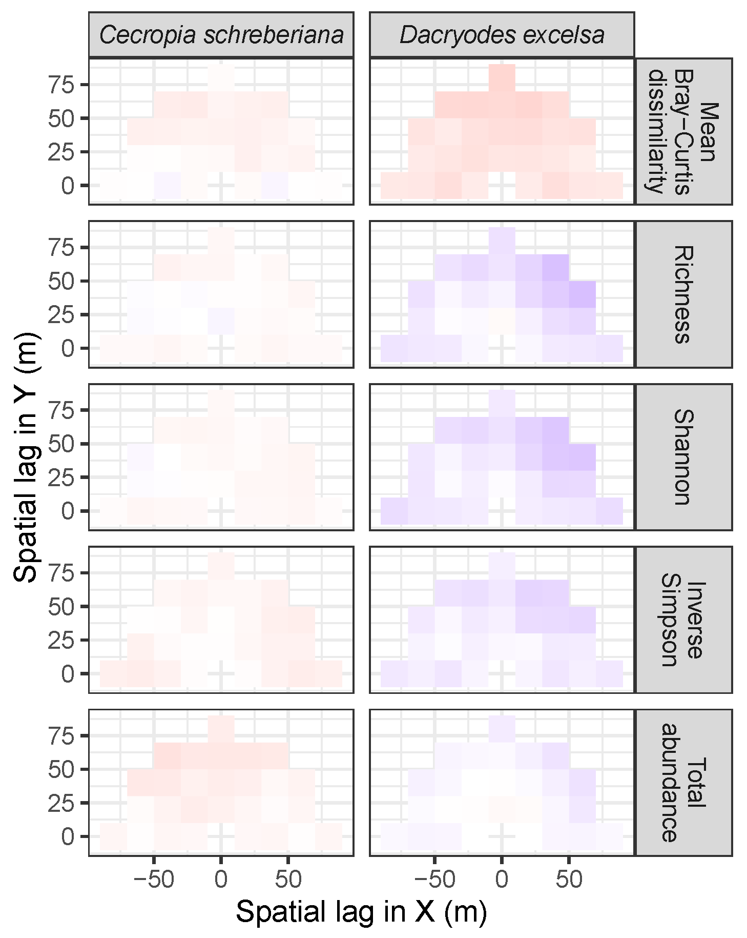
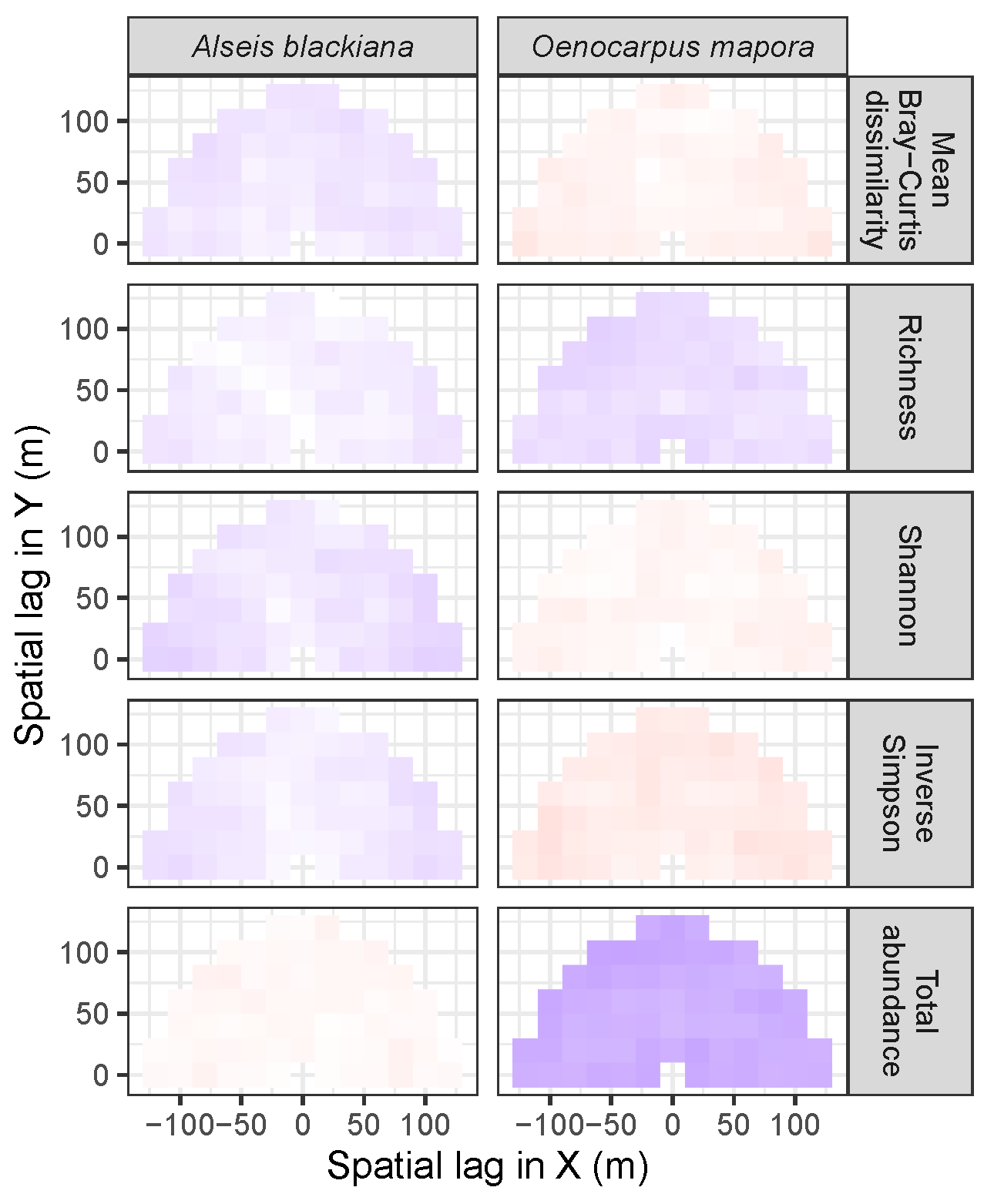
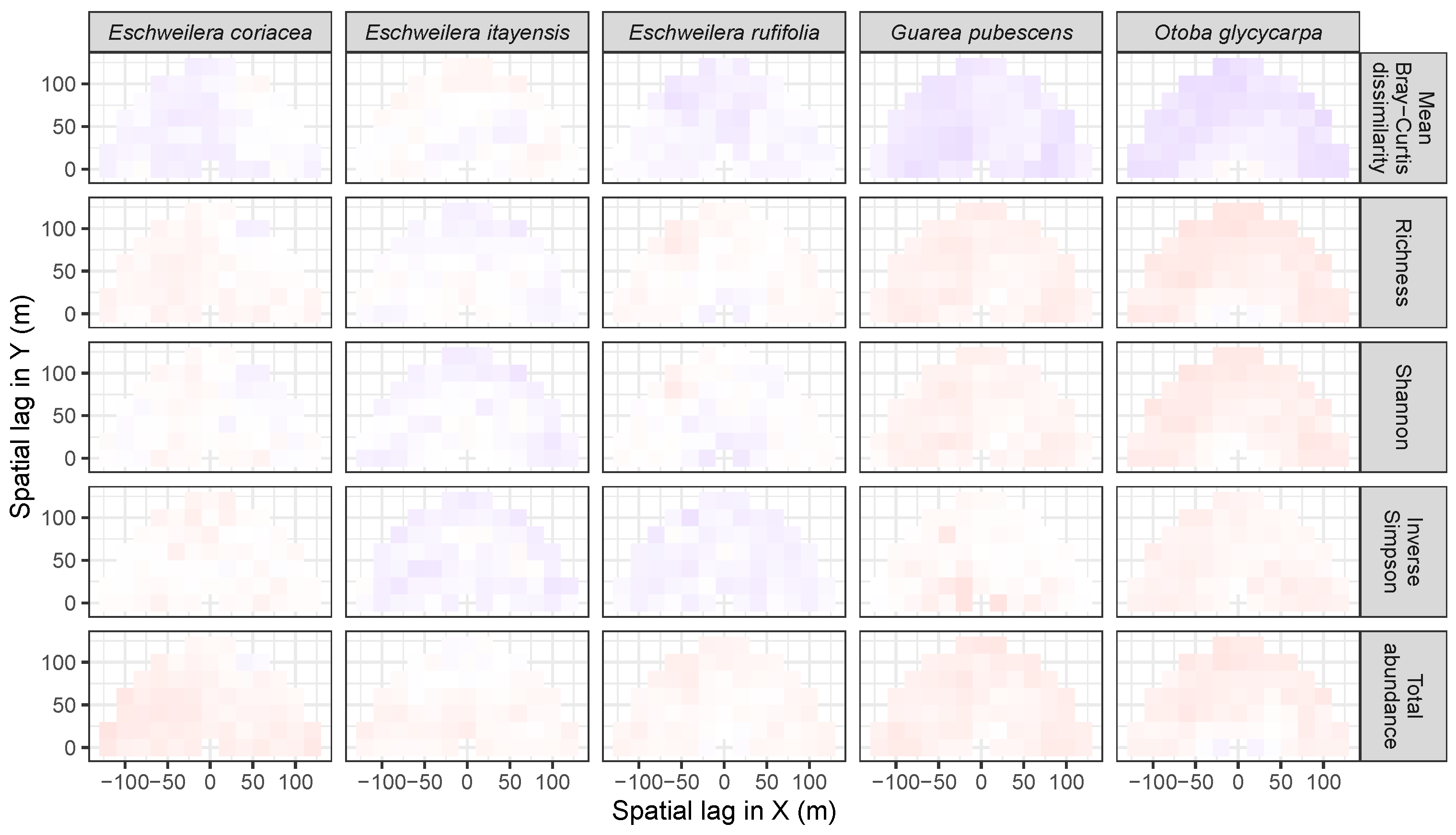
3.3.2. Trees at Tropical Sites

Codispersion between tree size or abundance and measures of associated-species diversity at the three tropical sites were much weaker than at the temperate sites (Figure 15, Figure 16 and Figure 17), and were less frequently statistically significant for most spatial lags or directions (Figure 18, Figure 19 and Figure 20 and Figure A3, Figure A4 and Figure A5). Notable exceptions included: positive codispersion between basal area of Dacryodes excelsa and Bray-Curtis dissimilarity at LFDP (Figure 15); negative codispersion between basal area of Oenocarpus mapora and associated-species richness and abundance at BCI (Figure 16); and positive codispersion between basal area of O. mapora and associated-species Simpson’s diversity at BCI (Figure 16). In all cases, however, values of codispersion were much less than that observed for Q. rubra at HF (except for codispersion between basal area of O. mapora and associated-species abundance, which was similar to that of Q. rubra at HF) (Table A2). At Amacayacu, the most species-rich site, total basal area of the dominant tree species had small and rarely significant spatial associations with metrics of diversity of associated woody species (Figure 17 and Figure 20 and Figure A5).

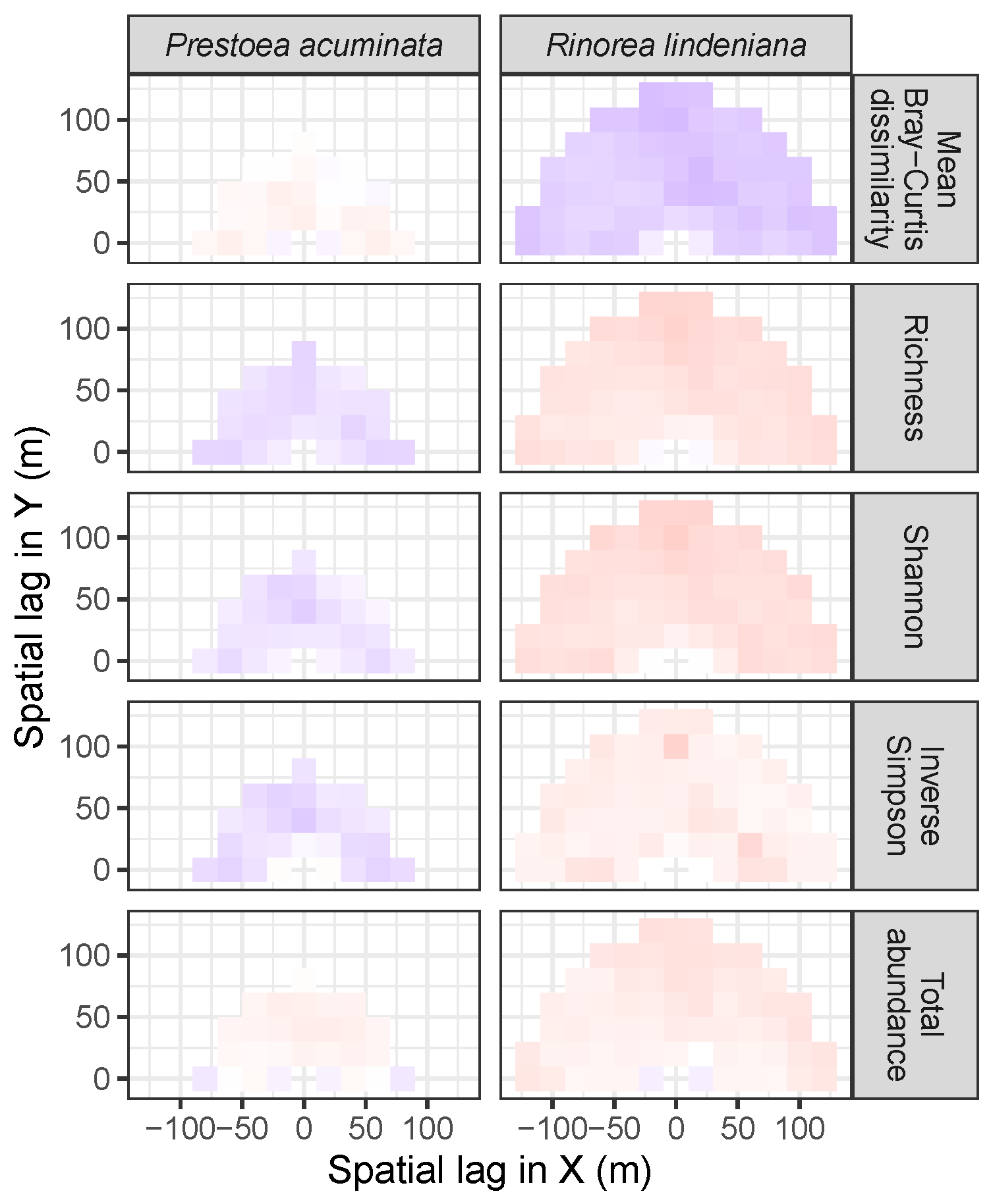
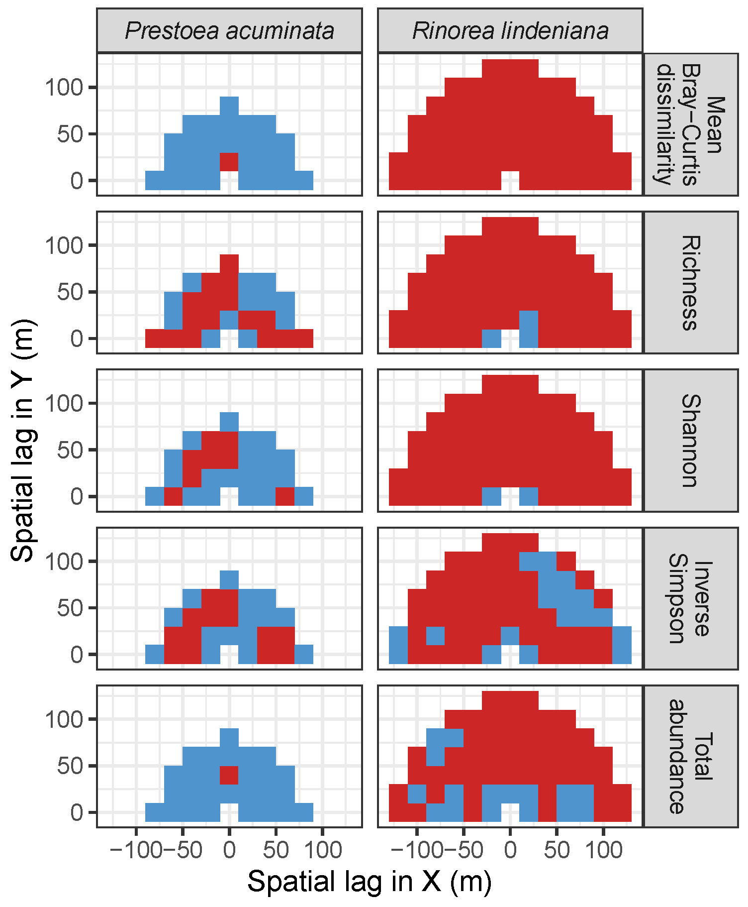
3.4. Codispersion Between Focal Understory Species and Associated-species Diversity

Understory species were included in our focal species list at two temperate sites (WR, TY) and two tropical sites (LFDP, AM) (Table 1; Figure A6, Figure A7, Figure A8, Figure A9, Figure A10 and Figure A11; Table A3 and Table A4). Of all of these, consistently significant codispersion between basal area and any metrics of associated-species diversity was observed only for Acer circinatum at WR, Cornus florida at TY, and Rinorea lindeniana at AM (Figure A10 and Figure A11). At WR, codispersion between basal area of A. circinatum and both Shannon and Simpson diversity was consistently negative, but was consistently positive with Bray-Curtis dissimilarity (Figure A6, Figure A7 and Figure A8). At AM, the pattern was reversed. There, codispersion between basal area of R. lindeniana and both Shannon and Simpson’s diversity were consistently positive, but was consistently negative with Bray-Curtis dissimilarity (Figure A9, Figure A10 and Figure A11), and were of the same magnitude or lower than that observed for Q. rubra at HF (Table A4). At TY, codispersion between basal area of C. florida and both associated-species richness and Bray-Curtis similarity were consistently negative (Figure A6 and of low magnitude (Table A3).

4. Discussion

Foundation species in forests define and structure entire ecological communities primarily through non-trophic effects such as providing physical points of attachment for associated species (e.g., epiphytes), creating habitat for associated fauna (e.g., tree-holes), modulating hydrological flow of adjacent streams, or altering the chemical composition of soils [2,3,52]. Forest foundation species most frequently are common, abundant, and large, and have been identified more frequently in temperate forests [2,53] than in tropical ones [2]. Ellison et al. [2] suggested that foundation tree species would be more likely in comparatively species-poor temperate forests because functional redundancy among trees there would be much less common than in species-rich tropical forests (e.g., [54,55]). In partial support of this idea, Lamanna et al. presented data showing a peak in the size of functional-trait space for tree assemblages growing at mid-latitudes (where our temperate plots are located) but more narrow functional-trait space for tropical assemblages [56]; see also [57]. These analyses imply that foundation tree species should be less common in very high latitude ecosystems (examined in more detail by [56] than by [57]). In those ecosystems, low-growing perennial, cushion- and tussock-forming plants have been found to be foundation species (e.g., [58]).
Indeed, the goal of testing community ecology’s neutral theory (which posits that differences among trophically similar species, such as trees, are irrelevant to their demographic success and subsequent spatial distribution), deriving from Hubbell’s work in a 13-ha plot in Costa Rica [59,60], in part motivated the establishment of the 50-ha plot at BCI in 1980 and subsequently other tropical forest dynamics plots. Although neutral theory has been supported for some distributional patterns in many tropical forests, it fails in others [61]. Niche theory (which posits functional non-equivalence of co-occurring, trophically similar species) more strongly fits data observed in temperate forests [62] and many tropical ones, too [61]. Thus, there is no a priori reason to suspect on functional grounds that foundation species should be less likely to occur in tropical forests than in temperate ones. We note also that the definition of foundation species [1,2] implicitly assumes that they always have non-neutral effects on the systems they define. However, it is plausible that the high abundance of these species causes them to have neutral influences on co-occurring species via ecological drift (i.e., by keeping local populations of associated species at low abundance, contributing to their demographic stochasticity). This might help explain why the basal area of the potential foundation species we examined was often negatively correlated with local species richness but positively correlated with beta diversity of associated species.
Despite the ecological importance of foundation species, it has proven challenging to identify plausible foundation species from among groups of locally dominant species or those that are perceived by various criteria to have importance in particular systems. It has taken decades of observational and experimental work to support the hypothesis that Tsuga canadensis is a foundation species in eastern North American forests [16] and that Pinus albicaulis is a foundation species in high-elevation western North American forests [53]. In both cases, their foundational characteristics were identified only as these species were declining [2]. If foundation species really are of critical importance for associated biodiversity, it is crucial that they be identified and protected while they are still common, locally abundant, and present in their full size distribution [6,27]. Because experiments on forest trees can take decades to centuries (and are generally impractical with longer-lived species), alternative approaches to identifying foundation forest species are needed.
Our statistical screening of abundance and size data from six large forest dynamics plots suggested particular characteristics of potential foundation species from two different size-frequency and diameter-abundance distributions (Figure 2, Figure 3, Figure 4 and Figure 5). The foundation species T. canadensis was a notable outlier from the “reverse-J” distribution of abundance versus mean diameter in the entire Harvard Forest 35-ha forest dynamics plot (Figure 2) and had a much greater range and spread of values of total basal area versus abundance in the 20-m rasterized plot (Figure 3). A similarly small set of species that had similar characteristics were identified in the other forest dynamics plots we analyzed (Figure 4 and Figure 5), with more candidates identified in the temperate plots than the tropical ones. This result is not especially surprising, as the more even abundance distributions of most tropical forests suggest that any species with both of these screening characteristics would be less common in the tropics. Alternatively, groups of species with similar traits (e.g., the Eschweilera species [Lecythidaceae] at AM, Dipterocarpaceae in Southeast Asia, or Quercus species at TY) or particular characteristics of individuals themselves (e.g., very large trees [26,27]) could have disproportionate influence akin to foundational characteristics in the forests in which they occur. This hypothesis is in need of additional exploration.
We also note that departures from the “reverse-J” size-frequency distribution may depend on when in succession a stand is sampled [63]. For example, abundance of early seral species (such as Pseudotsuga menziesii at WR) may initially be very abundant but relatively small. Because P. menziesii has been decreasing in abundance for at least the last 200 years at WR [64], it might be identified as a candidate foundation species in a 300-year-old stand, but not in the older forest dynamics plot at WR. That both the subcanopy A circinatum and the late-seral T. heterophylla basically mirror the position of P. menziesii in the size-frequency plot (Figure 4) adds some support for this hypothesis. Conversely, the foundational characteristics of T. heterophylla suggested by Figure 4 and Figure 5 might not yet be manifest this early in succession (cf. [63]). Related to this, some of the species that fall off the “reverse-J” have intermediate shade-tolerance and their role is likely to change during succession.
Subsequent analysis of spatial relationships between these candidate foundation species, along with others of known ecological importance (Table 1), and metrics of diversity of associated species pointed to attributes of T. canadensis shared by only a few other species. These included codispersion values > | 0.25 | at virtually all spatial lags and directions for two or more metrics of diversity that were often negative for measures of abundance or alpha-diversity (within-subplot species richness, Shannon diversity, or inverse-Simpson’s diversity) but positive for a measure of beta diversity (average subplot Bray-Curtis dissimilarity). That is, foundation species are negatively correlated with diversity of associated species at local (within-subplot) spatial scales where they dominate the vegetation but are positively associated with beta diversity at the larger (between subplot) spatial scale of the whole-plot. In virtually all cases (a notable exception being Pseudotsuga menziesii at WR), little effect of underlying environmental patchiness was observed: the toroidal-shift null model and the CSR null model gave nearly identical results, with the toroidal-shift null model being predictably more conservative.
By these criteria, candidates for additional, more detailed study for their foundational roles include Acer circinatum at WR, Dacryodes excelsa at Luquillo, and Oenocarpus mapora at BCI (Figure 15 and Figure 16 and Figure A6). In the western Cascades of Oregon, A. circinatum is a major component of the subcanopy, where it can grow rapidly, have high biomass, and form broad canopies that suppress other species [65,66]. This suppression of recruiting species could lead to negative association between A. circinatum basal area and local diversity of associated species (as is also seen with T. canadensis in eastern North American forests). At Luquillo, adult D. excelsa dominates ridges where trees form root grafts that may, in part, explain their relatively low hurricane mortality (<1%) [67,68]. Dacryodes excelsa saplings also grow more rapidly than saplings of other late successional species [68], which may explain the lack of pole-sized individuals in their populations [67]. Finally, O. mapora alters litter quality and quantity and the local microenvironment, and limits establishment of small-seeded and shade-intolerant species at BCI [69].
Disturbance frequency also may play a role in both statistical “fingerprints” of foundation species. For example, intermediate disturbance regimes (moderately frequent disturbances of moderate size and severity, such as small understory fires, multi-tree blowdowns, or selective harvesting) could push mid-successional, shade-intermediate species such as Q. rubra or A. rubrum at Harvard Forest back into the “reverse-J” distribution. At the same time, successional dynamics of these species (especially recruitment and prolonged growth) could result in transient conditions whereby they have both relatively high basal area and large numbers of small individuals in any given subplot. Where these species fall within the fingerprints, therefore, may indicate how their life-history traits are aligned with the frequency and type of local disturbances. How foundation species exert control on disturbance regimes in forests has not been previously explored. It would be useful to explore how positive feedbacks between a forest foundation species and local disturbances (especially fire, small windstorms or microbursts, and treefalls) could affect size-frequency and diameter-abundance distributions of associated species. These processes also are likely to differ in temperate and tropical forests (e.g., [70,71,72]).
Although local diversity of associated woody species is lower in the presence of foundation species, local diversity of other taxa associated with foundation species is often higher or composed of unique assemblages. Non-woody vascular and especially nonvascular plant taxa, and fauna are rarely sampled at the individual tree scale or in every 20 × 20-m subplot in large forest dynamics plots, but a handful of other studies have examined associations between these taxa and either T. canadensis or our candidate foundation species. For example, T. canadensis hosts unique assemblages of arthropods [73,74,75,76]. Acer circinatum is associated with a diverse and abundant assemblage of epiphytes [77]. At Luquillo, higher numbers of invertebrate species are associated with Dacryodes excelsa than with other dominant canopy species (including Cecropia schreberiana) [78], but abundances and herbivory rates of invertebrates on D. excelsa are lower than on other co-occurring species [79]. Several understory palms, including O. mapora, recently have been described as “terrestrial litter trappers” [80] that collect leaf litter at the base of their foliage. Two other litter-trapping palms, Asterogyne sociale and A. spectabilis, have very large numbers of arthropods in the trapped litter [81]; comparable studies with O. mapora would provide a useful comparison with the known and potential foundation species discussed here.
Finally, species like T. canadensis, P. menziesii and D. excelsa “name” their communities: hemlock, Douglas-fir, and tabonuco forests, respectively. The forest stands they dominate are easily identifiable as distinctive patches on the landscape. When a foundation species like T. canadensis declines, the associated regional or landscape-scale beta diversity is likely to decline along with it. Such regional homogenization—as indicated by lower Bray-Curtis values—is more characteristic of the majority of our focal species and would be a likely consequence of the loss of our candidate foundation species. It is precisely this larger-scale heterogeneity that may be the greatest value gained by protecting foundation species while they are still common.

5. Conclusions

Foundation species define and structure ecological communities but are difficult to identify before they are declining. Comparative analyses of six large forest dynamics plots spanning a temperate-to-tropical gradient in the Western Hemisphere identified statistical “fingerprints” of potential foundation species. Specifically, known and potential foundation species are outliers from the common “reverse-J” size-frequency distribution, and have negative effects on alpha diversity and positive effects on beta diversity at most spatial lags and directions. Potential foundation species appear to be more likely in temperate forests, whereas in tropical forests, foundational characteristics may be more likely to occur in species groups within genera or families. As foundation species (or species groups) decline, local (alpha) diversity may increase but landscape-scale (beta) diversity is likely to decline along with them. Preservation of beta biodiversity may be the most important consequence of protecting foundation species while they are still common.

Author Contributions

Conceptualization, A.M.E., H.L.B. and B.S.C.; statistical methodology, A.M.E., H.L.B. and B.S.C.; coding: H.L.B., B.S.C. and A.M.E.; forest dynamics plot establishment, data collection, and curation: D.C.; Á.J.D., J.A.L., J.A.M., D.A.O. and J.K.Z.; writing and editing, all authors.

Funding

This research was funded by the Smithsonian Institution, Utah State University, and the Utah Agricultural Experiment Station (projects 1153 and 1398) (WR plot); NSF grant 123749, the Smithsonian Institution, and the Harvard Forest (HF plot); Tyson Research Center, the International Center for Energy, Environment and Sustainability (InCEES) at Washington University in St. Louis, Smithsonian ForestGEO, and NSF grant DEB 1557094 (TY plot); the NSF-supported Luquillo Experimental Forest Long-Term Ecological Research Program, the University of Puerto Rico, and the International Institute of Tropical Forestry (LFDP plot); NSF grants 021104, 021115, 0212284, 0212818 and 0314581, and the Center for Tropical Forest Science (CTFS) (BCI plot); and Parques Nacionales Naturales de Colombia, Eliana Martínez and staff members of the Amacayacu Natural National Park, and the Center for Tropical Forest Science (CTFS) (AM plot).

Acknowledgments

An early version of this paper was presented at the 2014 International LTER meeting in Valdivia, Chile. We especially thank Ronny Vallejos for development of software to measure and plot codispersion, and for his continuing collegial collaboration with A.M.E., H.L.B., and B.S.C. Two anonymous reviewers provided helpful comments that substantially improved the final version of the paper. We acknowledge logistical support from the Gifford Pinchot National Forest, the USDA Forest Service Pacific Northwest Research Station, and the volunteers individually listed at http://wfdp.org for the WR plot. We also thank the many field technicians who helped census the HF plot; Jason Aylward for field supervision, data screening and database management at HF; and John Wisnewski and the Harvard Forest Woods Crew for providing materials, supplies, and invaluable field assistance with plot logistics. We thank the Tyson Research Center staff and more than 100 students and researchers that have contributed to tree censuses at TY. We sincerely thank the many volunteers who collected tree census data at LFDP. Vegetation data from BCI are part of the BCI forest dynamics research project founded by S.P. Hubbell and R.B. Foster and now managed by R. Condit, S. Lao, and R. Pérez through the Center for Tropical Forest Science (CTFS) and the Smithsonian Tropical Research Institute (STRI) in Panamá. We are very grateful for the assistance of coworkers from the Comunidad de Palmeras and the students of forest engineering from the Universidad Nacional de Colombia who collected tree census data at the AM plot. This paper is a contribution of the Harvard Forest and Luquillo LTER programs.

Conflicts of Interest

The authors declare no conflict of interest. The funders had no role in the design of the study; in the collection, analyses, or interpretation of data; in the writing of the manuscript, or in the decision to publish the results.

Appendix A. Supplemental Tables and Figures

Table A1. Codispersion statistics for focal tree species in temperate forests (Figure 8, Figure 9, Figure 10, Figure 11, Figure 12, Figure 13, Figure 14, Figure 15, Figure 16, Figure 17, Figure 18, Figure 19, Figure 20 and Figure A1 and Figure A2).
SiteSpeciesDiversity MetricMinMedianMean (SD)Max
WRPseudotsuga menzeisiiBray-Curtis0.050.110.11 (0.02)0.15
Richness−0.21−0.14−0.13 (0.05)−0.06
Shannon−0.15−0.07−0.07 (0.04)0.02
Simpson−0.08−0.010 (0.04)0.08
Abundance−0.11−0.03−0.04 (0.04)0.03
Tsuga heterophyllaBray−Curtis−0.040.010.01 (0.03)0.06
Richness−0.31−0.27−0.27 (0.03)−0.21
Shannon−0.13−0.09−0.09 (0.03)−0.03
Simpson−0.09−0.04−0.04 (0.03)0.03
Abundance−0.47−0.44−0.43 (0.03)−0.35
Abies amabilisBray−Curtis−0.140.030.02 (0.04)0.07
Richness0.040.090.1 (0.04)0.17
Shannon−0.020.010.02 (0.03)0.08
Simpson−0.060.010 (0.03)0.06
Abundance0.030.130.13 (0.04)0.19
HFAcer rubrumBray−Curtis0.010.060.07 (0.03)0.13
Richness−0.010.110.11 (0.04)0.19
Shannon−0.050.050.05 (0.03)0.11
Simpson−0.040.070.07 (0.04)0.14
Abundance−0.06−0.010 (0.02)0.05
Pinus strobusBray−Curtis−0.1−0.04−0.04 (0.04)0.07
Richness−0.09−0.010 (0.05)0.09
Shannon−0.060.030.02 (0.04)0.09
Simpson−0.030.070.07 (0.05)0.17
Abundance−0.21−0.09−0.11 (0.06)−0.02
Quercus rubraBray−Curtis−0.28−0.21−0.2 (0.05)−0.07
Richness−0.2−0.11−0.12 (0.05)0
Shannon−0.1100 (0.06)0.12
Simpson−0.050.090.09 (0.08)0.24
Abundance−0.4−0.28−0.27 (0.07)−0.1
Tsuga canadensisBray−Curtis0.120.210.21 (0.05)0.28
Richness−0.64−0.49−0.49 (0.08)−0.29
Shannon−0.46−0.34−0.34 (0.07)−0.17
Simpson−0.26−0.2−0.2 (0.04)−0.07
Abundance−0.45−0.33−0.34 (0.06)−0.24
TYQuercus albaBray−Curtis−0.27−0.18−0.18 (0.05)−0.04
Richness−0.24−0.18−0.18 (0.03)−0.12
Shannon−0.16−0.08−0.08 (0.04)0.01
Simpson−0.13−0.03−0.03 (0.05)0.05
Abundance−0.26−0.18−0.19 (0.05)−0.09
Quercus rubraBray−Curtis−0.18−0.08−0.09 (0.05)0
Richness−0.55−0.39−0.39 (0.1)−0.21
Shannon−0.29−0.23−0.22 (0.05)−0.09
Simpson−0.2−0.1−0.09 (0.06)0.07
Abundance−0.42−0.21−0.22 (0.1)−0.05
Quercus velutinaBray−Curtis−0.16−0.08−0.07 (0.04)0.06
Richness−0.140−0.01 (0.06)0.1
Shannon0.020.10.1 (0.04)0.17
Simpson−0.010.130.13 (0.05)0.22
Abundance−0.28−0.14−0.15 (0.07)−0.01
Carya glabraBray−Curtis−0.060.060.05 (0.04)0.12
Richness−0.050.050.06 (0.07)0.22
Shannon−0.16−0.06−0.07 (0.04)0.04
Simpson−0.26−0.18−0.16 (0.05)0
Abundance−0.090.110.09 (0.1)0.25
Carya ovataBray−Curtis0.040.150.14 (0.04)0.22
Richness−0.10.080.07 (0.06)0.17
Shannon−0.13−0.02−0.02 (0.04)0.07
Simpson−0.13−0.05−0.06 (0.03)0.03
Abundance−0.070.030.03 (0.05)0.13
Carya tomentosaBray−Curtis−0.12−0.04−0.04 (0.05)0.08
Richness−0.050.050.05 (0.05)0.18
Shannon−0.19−0.04−0.06 (0.05)0.04
Simpson−0.26−0.07−0.09 (0.08)0.02
Abundance−0.030.120.12 (0.1)0.35
Table A2. Codispersion statistics for focal tree species in tropical forests (Figure 15, Figure 16, Figure 17, Figure 18, Figure 19, Figure 20 and Figure A1, Figure A2, Figure A3, Figure A4 and Figure A5).
SiteSpeciesDiversity MetricMinMedianMean (SD)Max
Richness−0.040.040.03 (0.03)0.09
Shannon−0.030.050.04 (0.03)0.07
Simpson0.010.070.06 (0.04)0.12
Abundance0.010.080.09 (0.05)0.2
Dacryodes excelsaBray−Curtis0.120.190.19 (0.05)0.28
Richness−0.28−0.11−0.11 (0.07)0.03
Shannon−0.24−0.1−0.12 (0.06)−0.02
Simpson−0.18−0.09−0.09 (0.05)−0.01
Abundance−0.12−0.03−0.03 (0.04)0.04
BCIAlseis blackianaBray−Curtis−0.15−0.11−0.1 (0.02)−0.05
Richness−0.12−0.07−0.07 (0.03)0.01
Shannon−0.19−0.12−0.12 (0.04)−0.03
Simpson−0.16−0.09−0.09 (0.03)−0.02
Abundance0.010.050.05 (0.02)0.1
Oenocarpus maporaBray−Curtis0.010.080.08 (0.03)0.17
Richness−0.2−0.14−0.14 (0.02)−0.08
Shannon−0.010.060.06 (0.03)0.11
Simpson0.080.130.14 (0.03)0.2
Abundance−0.39−0.34−0.34 (0.02)−0.3
AMEschweilera coriaceaBray−Curtis−0.09−0.05−0.04 (0.03)0.06
Richness−0.070.050.04 (0.03)0.09
Shannon−0.060.010.01 (0.03)0.08
Simpson−0.020.020.03 (0.03)0.11
Abundance−0.040.090.09 (0.04)0.18
Eschweilera itayensisBray−Curtis−0.060.020.02 (0.03)0.09
Richness−0.09−0.02−0.01 (0.03)0.06
Shannon−0.11−0.03−0.03 (0.03)0.03
Simpson−0.1−0.05−0.04 (0.03)0.04
Abundance−0.020.040.04 (0.03)0.12
Eschweilera rufifoliaBray−Curtis−0.12−0.04−0.05 (0.03)0.01
Richness−0.060.030.03 (0.04)0.13
Shannon−0.090.010 (0.04)0.13
Simpson−0.12−0.05−0.05 (0.02)0.02
Abundance−0.020.050.05 (0.03)0.12
Guarea pubescensBray−Curtis−0.14−0.09−0.09 (0.03)−0.04
Richness−0.010.090.09 (0.03)0.14
Shannon00.080.08 (0.03)0.15
Simpson−0.010.030.04 (0.04)0.18
Abundance0.010.10.1 (0.03)0.17
Otoba glycarpaBray−Curtis−0.16−0.11−0.1 (0.04)0.04
Richness−0.020.130.11 (0.05)0.19
Shannon00.110.11 (0.04)0.17
Simpson00.070.07 (0.03)0.13
Abundance−0.050.10.09 (0.05)0.17
Figure A1. Statistical significance (red: P 0.05 ; blue: P > 0.05 ) of the codispersion coefficients calculated between measures of diversity and total basal area of the four dominant species in 20 × 20-m subplots in the 25.6-ha Wind River plot (Figure 11). Statistical significance was determined by comparing observed codispersion at each spatial lag with a distribution of 199 spatial randomizations of a CSR null model.
Forests 10 00128 g0a1
Figure A2. Statistical significance (red: P 0.05 ; blue: P > 0.05 ) of the codispersion coefficients calculated between measures of diversity and total basal area of the six focal tree species in 20 × 20-m subplots in the 20-ha Tyson Research Center plot (Figure 13). Statistical significance was determined by comparing observed codispersion at each spatial lag with a distribution of 199 spatial randomizations of a CSR null model.
Forests 10 00128 g0a2
Figure A3. Statistical significance (red: P 0.05 ; blue: P > 0.05 ) of the codispersion coefficients calculated between measures of diversity and total basal area of the two focal tree species in 20 × 20-m subplots in the 16-ha Luquillo plot (Figure 15). Statistical significance was determined by comparing observed codispersion at each spatial lag with a distribution of 199 spatial randomizations of a CSR null model.
Forests 10 00128 g0a3
Figure A4. Statistical significance (red: P 0.05 ; blue: P > 0.05 ) of the codispersion coefficients calculated between measures of diversity and total basal area of the two focal tree species in 20 × 20-m subplots in the 50-ha BCI plot (Figure 16). Statistical significance was determined by comparing observed codispersion at each spatial lag with a distribution of 199 spatial randomizations of a CSR null model.
Forests 10 00128 g0a4
Figure A5. Statistical significance (red: P 0.05 ; blue: P > 0.05 ) of the codispersion coefficients calculated between measures of diversity and total basal area of the five focal tree species in 20 × 20-m subplots in the 25-ha Amacayacu plot (Figure 17). Statistical significance was determined by comparing observed codispersion at each spatial lag with a distribution of 199 spatial randomizations of a CSR null model.
Forests 10 00128 g0a5
Figure A6. Codispersion between measures of diversity and total basal area of the focal understory species in 20 × 20-m subplots in the 25.6-ha Wind River (Acer circinatum, Taxus brevifolia) and 20-ha Tyson Research Center (Asimina triloba, Cornus florida, Frangula caroliniana, Lindera benzoin) plots. Codispersion coefficients were calculated for spatial lags ranging from 0–80 m (WR) and 0–105 (TY) at 20-m intervals. The value of the codispersion coefficient can range from 1 (dark blue) through 0 (white) to 1 (dark red). Statistical significance of each codispersion coefficient is shown in Figure A7 and Figure A8.
Forests 10 00128 g0a6
Figure A7. Statistical significance (red: P 0.05 ; blue: P > 0.05 ) of the codispersion coefficients calculated between measures of diversity and total basal area of the focal understory species in 20 × 20-m subplots in the 25.6-ha Wind River (Acer circinatum, Taxus brevifolia) and 20-ha Tyson Research Center (Asimina triloba, Cornus florida, Frangula caroliniana, Lindera benzoin) plots (Figure A6). Statistical significance was determined by comparing observed codispersion at each spatial lag with a distribution of 199 spatial randomizations of a toroidal shift model.
Forests 10 00128 g0a7
Figure A8. Statistical significance (red: P 0.05 ; blue: P > 0.05 ) of the codispersion coefficients calculated between measures of diversity and total basal area of the focal understory species in 20 × 20-m subplots in the 25.6-ha Wind River (Acer circinatum, Taxus brevifolia) and 20-ha Tyson Research Center (Asimina triloba, Cornus florida, Frangula caroliniana, Lindera benzoin) plots (Figure A6). Statistical significance was determined by comparing observed codispersion at each spatial lag with a distribution of 199 spatial randomizations of a CSR null model.
Forests 10 00128 g0a8
Figure A9. Codispersion between measures of diversity and total basal area of the focal understory species in 20 × 20-m subplots in the 16-ha Luquillo (Prestoea acuminata) and 25-ha Amacayacu (Rinorea lindeniana) plots. Codispersion coefficients were calculated for spatial lags ranging from 0–80 m (LFDP) and 0–125 (AM) at 20-m intervals. The value of the codispersion coefficient can range from 1 (dark blue) through 0 (white) to 1 (dark red). Statistical significance of each codispersion coefficient is shown in Figure A10 and Figure A11.
Forests 10 00128 g0a9
Figure A10. Statistical significance (red: P 0.05 ; blue: P > 0.05 ) of the codispersion coefficients calculated between measures of diversity and total basal area of the focal understory species in 20 × 20-m subplots in the 16-ha Luquillo (Prestoea acuminata) and 25-ha Amacayacu (Rinorea lindeniana) plots (Figure A9). Statistical significance was determined by comparing observed codispersion at each spatial lag with a distribution of 199 spatial randomizations of a toroidal-shift null model.
Forests 10 00128 g0a10
Figure A11. Statistical significance (red: P 0.05 ; blue: P > 0.05 ) of the codispersion coefficients calculated between measures of diversity and total basal area of the focal understory species in 20 × 20-m subplots in the 16-ha Luquillo (Prestoea acuminata) and 25-ha Amacayacu (Rinorea lindeniana) plots (Figure A9). Statistical significance was determined by comparing observed codispersion at each spatial lag with a distribution of 199 spatial randomizations of a CSR null model.
Forests 10 00128 g0a11
Table A3. Codispersion statistics for focal understory species in temperate forests (Figure A6, Figure A7 and Figure A8).
SiteSpeciesDiversity MetricMinMedianMean (SD)Max
WRAcer circinatumBray-Curtis0.170.220.22 (0.03)0.29
Richness0.030.090.08 (0.03)0.14
Shannon0.10.140.15 (0.04)0.25
Simpson0.10.140.16 (0.05)0.26
Abundance−0.27−0.12−0.14 (0.05)−0.06
Taxus brevifoliaBray−Curtis0.040.140.13 (0.05)0.22
Richness0.010.070.07 (0.03)0.11
Shannon0.020.050.06 (0.03)0.1
Simpson00.050.05 (0.03)0.12
Abundance0.030.120.11 (0.04)0.17
TYAsimina trilobaBray−Curtis0.050.160.15 (0.05)0.25
Richness0.020.080.08 (0.04)0.16
Shannon−0.120.010.02 (0.06)0.11
Simpson−0.18−0.05−0.04 (0.07)0.09
Abundance−0.170.030.01 (0.11)0.18
Cornus floridaBray−Curtis−0.27−0.13−0.14 (0.04)−0.05
Richness−0.26−0.22−0.21 (0.04)−0.07
Shannon−0.31−0.15−0.16 (0.07)−0.02
Simpson−0.2−0.07−0.08 (0.06)0.03
Abundance−0.11−0.03−0.03 (0.04)0.04
Frangula carolinianaBray−Curtis−0.040.080.07 (0.05)0.16
Richness−0.070.050.07 (0.1)0.24
Shannon−0.1−0.010 (0.06)0.11
Simpson−0.2−0.01−0.04 (0.06)0.07
Abundance−0.13−0.02−0.02 (0.07)0.16
Lindera benzoinBray−Curtis0.020.210.18 (0.09)0.33
Richness−0.040.10.11 (0.08)0.25
Shannon0.020.080.08 (0.03)0.13
Simpson−0.100 (0.05)0.07
Abundance−0.10−0.01 (0.05)0.08
Table A4. Codispersion statistics for focal understory species in tropical forests (Figure A9, Figure A10 and Figure A11).
SiteSpeciesDiversity MetricMinMedianMean (SD)Max
LFDPPrestoea acuminataBray-Curtis−0.040.050.04 (0.05)0.11
Richness−0.18−0.13−0.14 (0.03)−0.08
Shannon−0.2−0.1−0.11 (0.04)−0.05
Simpson−0.22−0.13−0.12 (0.06)0.02
Abundance−0.10.070.05 (0.06)0.13
AMRinorea lindenianaBray−Curtis−0.29−0.22−0.22 (0.04)−0.08
Richness−0.020.190.19 (0.06)0.3
Shannon0.010.210.21 (0.05)0.33
Simpson00.10.11 (0.05)0.3
Abundance−0.070.120.12 (0.06)0.21

References

  1. Dayton, P.K. Toward an understanding of community resilience and the potential effects of enrichments to the benthos at McMurdo Sound, Antarctica. In Proceedings of the Colloquium on Conservation Problems in Antarctica, Blacksburg, VA, USA, 10–12 September 1971; Parker, B.C., Ed.; Allen Press: Lawrence, KS, USA, 1972; pp. 81–95. [Google Scholar]
  2. Ellison, A.M.; Bank, M.S.; Clinton, B.D.; Colburn, E.A.; Elliott, K.; Ford, C.R.; Foster, D.R.; Kloeppel, B.D.; Knoepp, J.D.; Lovett, G.M.; et al. Loss of foundation species: Consequences for the structure and dynamics of forested ecosystems. Front. Ecol. Environ. 2005, 9, 479–486. [Google Scholar] [CrossRef]
  3. Baiser, B.; Whitaker, N.; Ellison, A.M. Modeling foundation species in food webs. Ecosphere 2013, 4, 146. [Google Scholar] [CrossRef]
  4. Gaston, K.J.; Fuller, R.A. Biodiversity and extinction: losing the common and the widespread. Prog. Phys. Geog. 2007, 31, 213–225. [Google Scholar] [CrossRef]
  5. Gaston, K.J.; Fuller, R.A. Commonness, population depletion and conservation biology. Trends Ecol. Evol. 2008, 23, 14–19. [Google Scholar] [CrossRef]
  6. Ellison, A.M.; Degrassi, A.L. All species are important, but some species are more important than others (Commentary). J. Veg. Sci. 2017, 28, 669–671. [Google Scholar] [CrossRef]
  7. Paine, R.T. Food web complexity and species diversity. Am. Nat. 1966, 100, 65–75. [Google Scholar] [CrossRef]
  8. Valls, A.; Coll, M.; Christensen, V. Keystone species: Toward an operational concept for marine biodiversity conservation. Ecol. Monogr. 2015, 85, 29–47. [Google Scholar] [CrossRef]
  9. Grime, J.P. Dominant and subordinate components of plant communities: implications for succession, stability and diversity. In Colonization, Succession and Stability; Gray, A.J., Crawley, M.J., Edwards, P.J., Eds.; Blackwell Scientific Publications: Oxford, UK, 1987; pp. 413–428. [Google Scholar]
  10. Leakey, R.; Lewin, R. The Sixth Extinction: Patterns of Life and the Future of Humankind; Anchor Books: New York, NY, USA, 1996. [Google Scholar]
  11. Short, F.; Carruthers, T.; Dennison, W.; Waycott, M. Global seagrass distribution and diversity: A bioregional model. J. Exp. Mar. Biol. Ecol. 2007, 350, 3–20. [Google Scholar] [CrossRef]
  12. Fischer, M.; Bossdorf, O.; Gockel, S.; Hänsel, F.; Hemp, A.; Hessenmöller, D.; Korte, G.; Nieschulze, J.; Pfeiffer, S.; Prati, D.; et al. Implementing large-scale and long-term functional biodiversity research: The Biodiversity Exploratories. Basic Appl. Ecol. 2010, 11, 473–485. [Google Scholar] [CrossRef]
  13. LaManna, J.A.; Mangan, S.A.; Alonso, A.; Bourg, N.A.; Brockelman, W.Y.; Bunyavejchewin, S.; Chang, L.-W.; Chiang, J.-M.; Chuyong, G.B.; Clay, K.; et al. Plant diversity increases with the strength of negative density dependence at the global scale. Science 2017, 356, 1389–1392. [Google Scholar] [CrossRef]
  14. ReefBase. ReefBase—A Global Information System on Coral Reefs. 2018. Available online: http://www.reefabase.org (accessed on 5 October 2018).
  15. Ellison, A.M.; Barker Plotkin, A.A.; Khalid, S. Foundation species loss and biodiversity of the herbaceous layer in New England forests. Forests 2016, 7, 9. [Google Scholar] [CrossRef]
  16. Ellison, A.M. Experiments are revealing a foundation species: A case study of eastern hemlock (Tsuga canadensis). Adv. Ecol. 2014, 2014, 456904. [Google Scholar] [CrossRef]
  17. Foster, D.R. (Ed.) Hemlock: A Forest Giant on the Edge; Yale University Press: New Haven, CT, USA, 2014. [Google Scholar]
  18. Orwig, D.A.; Barker Plotkin, A.A.; Davidson, E.A.; Lux, H.; Savage, K.E.; Ellison, A.M. Foundation species loss affects vegetation structure more than ecosystem function in a northeastern USA forest. PeerJ 2013, 1, e41. [Google Scholar] [CrossRef] [PubMed]
  19. Cuevas, F.; Porcu, E.; Vallejos, R. Study of spatial relationships between two sets off variables: A nonparametric approach. J. Nonparametr. Statist. 2013, 25, 695–714. [Google Scholar] [CrossRef]
  20. Buckley, H.L.; Case, B.S.; Ellison, A.M. Using codispersion analysis to characterize spatial patterns in species co-occurrences. Ecology 2016, 97, 32–39. [Google Scholar] [CrossRef] [PubMed]
  21. Buckley, H.L.; Case, B.S.; Zimmermann, J.; Thompson, J.; Myers, J.A.; Ellison, A.M. Using codispersion analysis to quantify and understand spatial patterns in species-environment relationships. New Phytol. 2016, 211, 735–749. [Google Scholar] [CrossRef] [PubMed]
  22. Case, B.S.; Buckley, H.L.; Barker Plotkin, A.; Ellison, A.M. Using codispersion analysis to quantify temporal changes in the spatial pattern of forest stand structure. Chil. J. Stat. 2016, 7, 3–15. [Google Scholar]
  23. Case, B.S.; Buckley, H.L.; Barker Plotkin, A.A.; Orwig, D.A.; Ellison, A.M. When a foundation crumbles: Forecasting forest community dynamics associated with the decline of the foundation species. Ecosphere 2017, 8, e01893. [Google Scholar] [CrossRef]
  24. Anderson-Teixeira, K.J.; Davies, S.J.; Bennett, A.C.; Gonzalez-Akre, E.B.; Muller-Landau, H.C.; Wright, S.J.; Abu Salim, K.; Almeyda Zambrano, A.M.; Alonso, A.; Baltzer, J.L.; et al. CTFS—ForestGEO: A worldwide network monitoring forests in an era of global change. Glob. Change Biol. 2015, 21, 528–549. [Google Scholar] [CrossRef]
  25. Condit, R. Tropical Forest Census Plots: Methods and Results from Barro Colorado Island, Panama and a Comparison with Other Plots; Springer: Berlin, Germany, 1998. [Google Scholar]
  26. Lutz, J.A.; Larson, A.J.; Freund, J.A.; Swanson, M.E.; Bible, K.J. The importance of large-diameter trees to forest structural heterogeneity. PLoS ONE 2013, 8, e82784. [Google Scholar] [CrossRef]
  27. Lutz, J.A.; Furniss, T.J.; Johnson, D.J.; Davies, S.J.; Allen, D.; Alonso, A.; Anderson-Teixeira, K.; Andrade, A.; Baltzer, J.; Becker, K.M.L.; et al. Global importance of large-diameter trees. Global Ecol. Biogeogr. 2018, 27, 849–864. [Google Scholar] [CrossRef]
  28. Das, A.J.; Larson, A.J.; Lutz, J.A. Individual species-area relationships in temperate coniferous forests. J. Veg. Sci. 2018, 29, 317–324. [Google Scholar] [CrossRef]
  29. Lutz, J.A.; Larson, A.J.; Furniss, T.J.; Freund, J.A.; Swanson, M.E.; Donato, D.C.; Bible, K.J.; Chen, J.; Franklin, J.F. Spatially non-random tree mortality and ingrowth maintain equilibrium pattern in an old-growth Pseudotsuga-Tsuga forest. Ecology 2014, 95, 2047–2054. [Google Scholar] [CrossRef] [PubMed]
  30. Griffith, G.E.; Omernik, J.M.; Pierson, S.M.; Kiilsgaard, C.W. The Massachusetts Ecological Regions Project; U.S. Environmental Protection Agency: Corvallis, OR, USA, 1994.
  31. Westveld, M.; Ashman, R.I.; Baldwin, H.I.; Holdsworth, R.P.; Johnson, R.S.; Lambert, J.H.; Lutz, H.J.; Swain, L.; Standish, M. Natural forest vegetation zones of New England. J. For. 1956, 54, 332–338. [Google Scholar]
  32. Wang, X.; Wiegand, T.; Anderson-Teixeira, K.J.; Bourg, N.A.; Hao, Z.; Howe, R.; Jin, G.; Orwig, D.A.; Spasojevic, M.J.; Wang, S.; et al. Ecological drivers of spatial community dissimilarity, species replacement and species nestedness across temperate forests. Global Ecol. Biogeogr. 2018, 27, 581–592. [Google Scholar] [CrossRef]
  33. Raup, H.M.; Carlson, R.E. The history of land use in the Harvard Forest. Harv. For. Bull. 1941, 20, 4–62. [Google Scholar]
  34. Foster, D.R. Land-use history (1730–1990) and vegetation dynamics in central New England, USA. J. Ecol. 1992, 80, 753–772. [Google Scholar] [CrossRef]
  35. Foster, D.R.; Zebryk, T.M.; Schoonmaker, P.K.; Lezberg, A.L. Post-settlement history of human land-use and vegetation dynamics of a hemlock woodlot in central New England. J. Ecol. 1992, 80, 773–786. [Google Scholar] [CrossRef]
  36. Spasojevic, M.J.; Yablon, E.A.; Oberle, B.; Myers, J.A. Ontogenetic trait variation influences tree community assembly across environmental gradients. Ecosphere 2014, 5, 129. [Google Scholar] [CrossRef]
  37. LaManna, J.A.; Walton, M.L.; Turner, B.L.; Myers, J.A. Negative density dependence is stronger in resource-rich environments and diversifies communities when stronger for common but not rare species. Ecol. Lett. 2016, 19, 657–667. [Google Scholar] [CrossRef]
  38. Zimmerman, M.; Wagner, W.L. A description of the woody vegetation of oak-hickory forest in the Northern Ozark Highlands. Bull. Torrey Bot. Club 1979, 106, 117–122. [Google Scholar] [CrossRef]
  39. Thompson, J.; Brokaw, N.; Zimmerman, J.K.; Waide, R.B.; Everham, E.M., III; Lodge, J.; Taylor, C.M.; Garca-Montiel, D.; Fluet, M. Land use history, environment, and tree composition in a tropical forest. Ecol. Appl. 2002, 12, 1344–1363. [Google Scholar] [CrossRef]
  40. Zimmerman, J.K.; Comita, L.S.; Thompson, J.; Uriarte, M.; Brokaw, N. Patch dynamics and community metastability of a tropical forest: Compound effects of natural disturbance and human land use. Landsc. Ecol. 2010, 25, 1099–1111. [Google Scholar] [CrossRef]
  41. Hogan, J.A.; Zimmerman, J.K.; Thompson, J.; Nytch, C.J.; Uriarte, M. The interaction of land-use legacies and hurricane disturbance in subtropical wet forest: Twenty-one years of change. Ecosphere 2016, 7, e01405. [Google Scholar] [CrossRef]
  42. Leigh, E.G., Jr.; Loo de Lao, S.; Condit, R.; Hubbell, S.P.; Foster, R.B.; Pérez, R. Barro Colorado Island Forest Dynamics Plot, Panama. In Tropical Forest Diversity and Dynamism: Findings from a Large-Scale Plot Network; Losos, E.C., Leigh, E.G., Jr., Eds.; University of Chicago Press: Chicago, IL, USA, 2004; pp. 451–463. [Google Scholar]
  43. Condit, R.; Pérez, R.; Lao, S.; Aguilar, S.; Hubbell, S.P. Demographic trends and climate over 35 years in the Barro Colorado 50 ha plot. For. Ecosyst. 2017, 4, 17. [Google Scholar] [CrossRef]
  44. Hubbell, S.P.; Foster, R.B.; O’Brien, S.T.; Harms, K.E.; Condit, R.; Wechsler, B.; Wright, S.J.; Loo de Lao, S. Light-gap disturbances, recruitment limitation, and tree diversity in a Neotropical forest. Science 1999, 283, 554–557. [Google Scholar] [CrossRef] [PubMed]
  45. Zuleta, D.; Russo, S.E.; Barona, A.; Barreto-Silva, J.S.; Carenas, D.; Castaño, N.; Davies, S.J.; Detto, M.; Sua, S.; Turner, B.L.; Duque, A. Importance of topography for tree species habitat distributions in a terra firme forest in the Colombian Amazon. Plant Soil 2018. [Google Scholar] [CrossRef]
  46. Loehle, C. Species abundance distributions result from body size-energetics relationships. Ecology 2006, 87, 2221–2226. [Google Scholar] [CrossRef]
  47. Chao, A.; Gotelli, N.J.; Hsieh, T.C.; Snader, E.L.; Ma, K.H.; Colwell, R.K.; Ellison, A.M. Rarefaction and extrapolation with Hill numbers: a framework for sampling and estimation in species diversity studies. Ecol. Monogr. 2014, 84, 45–67. [Google Scholar] [CrossRef]
  48. Bray, J.R.; Curtis, J.T. An ordination of upland forest communities of southern Wisconsin. Ecol. Monogr. 1957, 27, 325–349. [Google Scholar] [CrossRef]
  49. Oksanen, J.; Blanchet, F.G.; Friendly, M.; Kindt, R.; Legendre, P.; McGlinn, D.; Minchin, P.R.; O’Hara, R.B.; Simpson, G.L.; Solymos, P.; et al. Vegan: Community Ecology Package. R package version 2.5-3. Available online: https://CRAN.R-project.org/package=vegan (accessed on 3 February 2018).
  50. Vallejos, R.; Buckley, H.; Case, B.; Acosta, J.; Ellison, A.M. Sensitivity of codispersion to noise and error in ecological and environmental data. Forests 2018, 9, 679. [Google Scholar] [CrossRef]
  51. Osorio, F.; Vallejos, R.; Cuevas, F.; Mancilla, D. SpatialPack Package. R package version 0.3. Available online: https://cran.r-project.org/package=SpatialPack (accessed on 3 February 2018).
  52. Brantley, S.T.; Ford, C.R.; Vose, J.M. Future species composition will affect forest water use after loss of eastern hemlock from southern Appalachian forests. Ecol. Appl. 2013, 23, 777–790. [Google Scholar] [CrossRef] [PubMed]
  53. Tomback, D.F.; Resler, L.M.; Keane, R.E.; Pansing, E.R.; Andrade, A.J.; Wagner, A.C. Community structure, biodiversity, and ecosystem services in treeline whitebark pine communities: potential impacts from a non-native pathogen. Forests 2016, 7, 21. [Google Scholar] [CrossRef]
  54. Whitmore, T.C. Tropical Rain Forests of the Far East; Clarendon: Oxford, UK, 1984. [Google Scholar]
  55. Iwasa, Y.; Kubo, T.; Sato, K. Maintenance of forest species diversity and latitudinal gradient. Vegetatio 1995, 121, 127–134. [Google Scholar] [CrossRef]
  56. Lamanna, C.; Blonder, B.; Violle, C.; Kraft, N.J.B.; Sandel, B.; Šímová, I.; Donoghue, J.C., II; Svenning, J.-C.; McGill, B.J.; Boyle, B.; et al. Functional trait space and the latitudinal diversity gradient. Proc. Nat. Acad. Sci. USA 2014, 111, 13745–13750. [Google Scholar] [CrossRef] [PubMed]
  57. Wieczynski, D.J.; Boyle, B.; Buzzard, V.; Duran, S.M.; Henderson, A.N.; Hulshof, D.M.; Kerkhoff, A.J.; McCarthy, M.C.; Michaletz, S.T.; Swenson, N.G.; et al. Climate shapes and shifts functional biodiversity in forests worldwide. Proc. Nat. Acad. Sci. USA 2019, 116, 587–592. [Google Scholar] [CrossRef] [PubMed]
  58. Elumeeva, T.G.; Onipchenko, V.G.; Weger, M.J.A. No other species can replace them: evidence for the key role of dominants in an alpine Festuca varia grassland. J. Veg. Sci. 2017, 28, 674–683. [Google Scholar] [CrossRef]
  59. Hubbell, S.P. Tree dispersion, abundance, and diversity in a tropical dry forest. Science 1979, 203, 1299–1309. [Google Scholar] [CrossRef]
  60. Hubbell, S.P. The Unified Neutral Theory of Biodiversity and Biogeography; Princeton University Press: Princeton, NJ, USA, 2001. [Google Scholar]
  61. Leigh, E.G., Jr. Neutral theory: A historical perspective. J. Evol. Biol. 2007, 20, 2075–2091. [Google Scholar] [CrossRef]
  62. Furniss, T.J.; Larson, A.J.; Lutz, J.A. Reconciling niches and neutrality in a subalpine temperate forest. Ecosphere 2017, 8, e01847. [Google Scholar] [CrossRef]
  63. Ellison, A.M.; Lavine, M.; Kerson, P.B.; Barker Plotkin, A.A.; Orwig, D.A. Building a foundation: land-use history and dendrochronology reveal temporal dynamics of a Tsuga canadensis (Pinaceae) forest. Rhodora 2014, 116, 377–427. [Google Scholar] [CrossRef]
  64. Freund, J.A.; Franklin, J.F.; Lutz, J.A. Structure of early old-growth Douglas-fir forests in the Pacific Northwest. Forest Ecol. Manag. 2015, 335, 11–25. [Google Scholar] [CrossRef]
  65. Lutz, J.A.; Halpern, C.B. Tree mortality during early forest development: A long-term study of rates, causes, and consequences. Ecol. Monogr. 2006, 76, 257–275. [Google Scholar] [CrossRef]
  66. Halpern, C.B.; Lutz, J.A. Canopy closure exerts weak controls on understory dynamics: A 30-year study of overstory-understory interactions. Ecol. Monogr. 2013, 83, 221–237. [Google Scholar] [CrossRef]
  67. Basnet, K.; Scatena, F.N.; Likens, G.E.; Lugo, A.E. Ecological consequences of root grafting in tabonuco (Dacryodes excelsa) trees in the Luquillo Experimental Forest, Puerto Rico. Biotropica 1993, 25, 28–35. [Google Scholar] [CrossRef]
  68. Uriarte, M.; Canham, C.D.; Thompson, J.; Zimmerman, J.K. A neighborhood analysis of tree growth and survival in a hurricane-driven tropical forest. Ecol. Monogr. 2004, 74, 591–614. [Google Scholar] [CrossRef]
  69. Farris-Lopez, K.; Desnlow, J.S.; Moser, B.; Passmore, H. Influence of a common palm, Oenocarpus mapora on seedling establishment in a tropical moist forest in Panama. J. Trop. Ecol. 2004, 20, 429–438. [Google Scholar] [CrossRef]
  70. Baker, T.R.; Vela Díaz, D.M.; Chama Moscoso, V.; Navarro, G.; Monteagudo, A.; Pinto, R.; Cangani, K.; Fyllas, N.F.; Lopez Gonzalez, G.; Laurance, W.F.; et al. Consistent, small effects of treefall disturbances on the composition and diversity of four Amazonian forests. J. Ecol. 2016, 104, 497–506. [Google Scholar] [CrossRef]
  71. Battles, J.J.; Cleavitt, N.L.; Saah, D.S.; Pling, B.T.; Fahey, T.J. Ecological impact of a microburst windstorm in a northern hardwood forest. Can. J. For. Res. 2017, 47, 1695–1701. [Google Scholar] [CrossRef]
  72. Després, T.; Asselin, H.; Doyon, F.; Drobyshev, I.; Bergeron, Y. Gap dynamics of late successional sugar maple-yellow birch forests at their northern range limit. J. Veg. Sci. 2017, 28, 368–378. [Google Scholar] [CrossRef]
  73. Dilling, C.; Lambdin, P.; Grant, J.; Buck, L. Insect guild structure associated with eastern hemlock in the southern Appalachians. Env. Entomol. 2007, 36, 1408–1414. [Google Scholar] [CrossRef]
  74. Rohr, J.; Mahan, C.G.; Kim, K.C. Response of arthropod biodiversity to foundation species declines: the case of the eastern hemlock. Forest Ecol. Manag. 2009, 258, 1503–1510. [Google Scholar] [CrossRef]
  75. Sackett, T.E.; Record, S.; Bewick, S.; Baiser, B.; Sanders, N.J.; Ellison, A.M. Response of macroarthropod assemblages to the loss of hemlock (Tsuga canadensis), a foundation species. Ecosphere 2011, 2, e74. [Google Scholar] [CrossRef]
  76. Record, S.; McCabe, T.; Baiser, B.; Ellison, A.M. Identifying foundation species in North American forests using long-term data on ant assemblage structure. Ecosphere 2018, 9, e02139. [Google Scholar] [CrossRef]
  77. Ruchty, A.; Rosso, A.L.; McCune, B. Changes in epiphyte communities as the shrub, Acer circinatum, develops and ages. The Bryologist 2001, 104, 274–281. [Google Scholar] [CrossRef]
  78. Schowalter, T.D. Canopy invertebrate community response to disturbance and consequences of herbivory in temperate and tropical forests. Selbyana 1995, 16, 41–48. [Google Scholar]
  79. Schowalter, T.D. Invertebrate community structure and herbivory in a tropical rain forest canopy in Puerto Rico following Hurricane Hugo. Biotropica 1994, 26, 312–319. [Google Scholar] [CrossRef]
  80. Weissenhofer, A.; Huber, W.; Wanek, W.; Weber, A. Terrestrial litter trappers in the Golfo Dulce region: Diversity, architecture and ecology of a poorly known group of plant specialists. Stapfia 88, zugleich Kataloge der oberösterreichischen Landesmuseen (Neue Serie) 2008, 80, 143–154. [Google Scholar]
  81. De Vasconcelos, H.L. Effects of litter collection by understory palms on the associated macroinvertebrate fauna in Central Amazonia. Pedobiologia 1990, 34, 157–160. [Google Scholar]
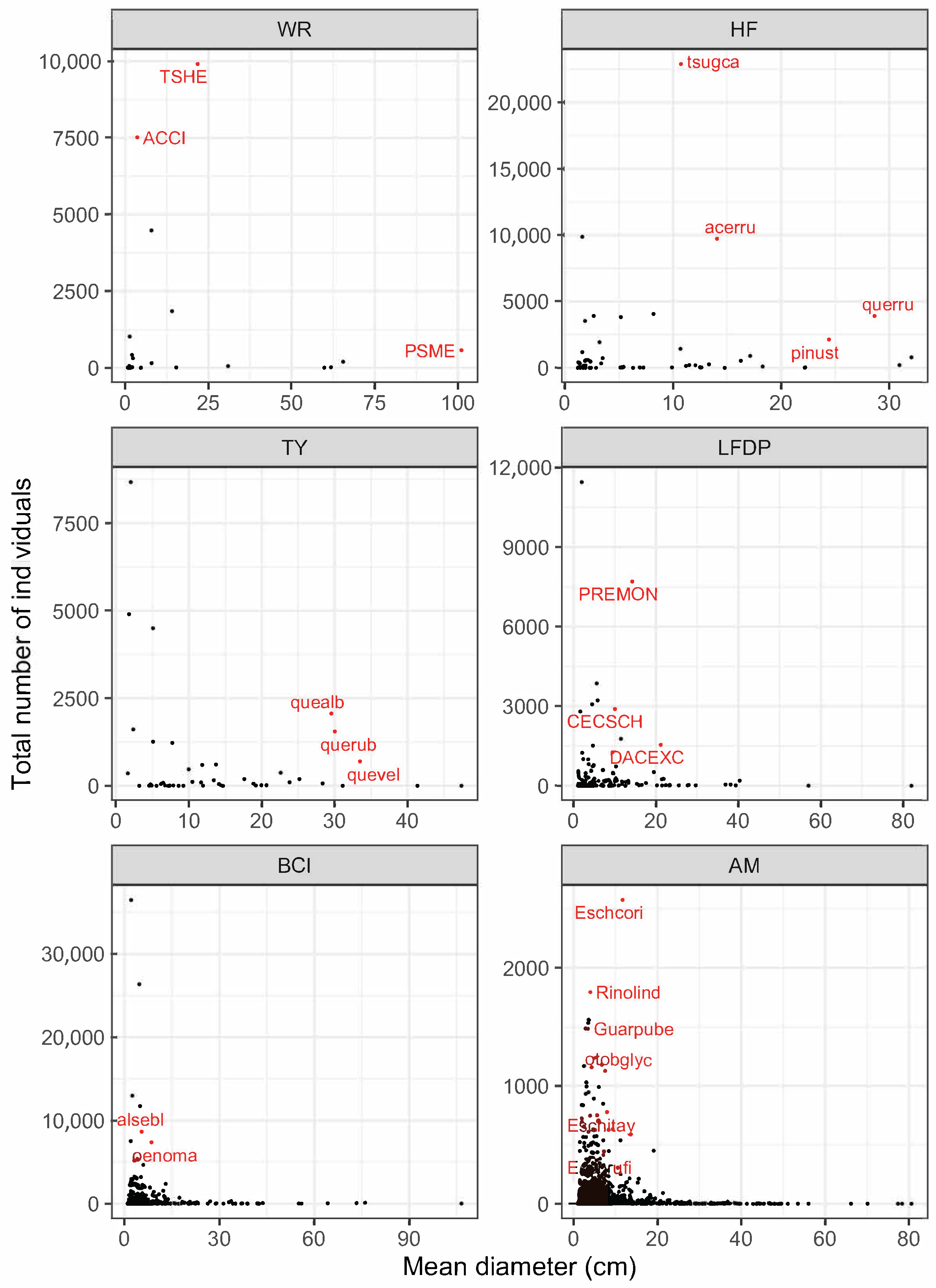
Figure 1. The geographic distribution of the six ForestGEO study sites we assessed for foundation species and their effects on diversity of associated woody plants. The size of the symbols are proportional to species richness of living woody species at each site: Wind River (20 species), Tyson (42), Harvard Forest (51), Luquillo (135), Barro Colorado Island (297), and Amacayacu (1232).
Forests 10 00128 g001
Figure 2. Size-frequency distribution of the 51 living woody species in the Harvard Forest 35-ha plot. Each point is the average diameter of all living stems ≥1-cm diameter for a single species. The four dominant species (labeled in red; key to abbreviations in Table 1) fall well away from the expected “reverse-J” distribution.
Forests 10 00128 g002
Figure 3. Total basal area and abundance (per 20 × 20-m subplot) of the four dominant species in the Harvard Forest 35-ha plot. Species abbreviations are given in Table 1.
Forests 10 00128 g003
Figure 4. Size-frequency distributions of the species in each of the six studied ForestGeo plots. Panels are ordered from the northernmost temperate (top left) to equatorial (bottom right). Species that do not lie on the “reverse-J” line or that were otherwise are thought to be “important” species (in the tropical plots) are identified in red. Species abbreviations are given in Table 1.
Forests 10 00128 g004
Figure 5. Total basal area and abundance (per 20 × 20-m subplot) of canopy tree species and two tropical understory species identified in Figure 4 as “important” in the six studied ForestGeo plots. Plots are ordered from the northernmost temperate (top left) to equatorial (bottom right). Species abbreviations are given in Table 1.
Forests 10 00128 g005
Figure 6. Abundance, total basal area, and mean basal area of all hypothesized foundation species and other focal species (Table 1) in the six 20-m rasterized forest dynamics plots. Sites are ordered top-to-bottom by decreasing latitude, and each plot is scaled relative to the 50-ha BCI plot. White squares in the BCI and AM panels indicate none of the focal species were present in that subplot.
Forests 10 00128 g006
Figure 7. Abundance, species richness, two measures of species diversity, and one measure of beta diversity for all species other than the focal species (Table 1) in the six 20-m rasterized forest dynamics plots. Sites are ordered top-to-bottom by decreasing latitude, and each plot is scaled relative to the 50-ha BCI plot. White squares in the WR, HF, and TY panels indicate that only the focal species were present in that subplot.
Forests 10 00128 g007
Figure 8. Codispersion between measures of diversity and total basal area of the four focal species in 20 × 20-m subplots in the 35-ha Harvard Forest plot. Codispersion coefficients were calculated for spatial lags ranging from 0–125 m at 20-m intervals. The value of the codispersion coefficient can range from −1 (dark blue) through 0 (white) to 1 (dark red). Statistical significance of each codispersion coefficient is shown in Figure 10. Summaries of codispersion values are given in Table A1).
Forests 10 00128 g008
Figure 9. Statistical significance (red: P 0.05 ; blue: P > 0.05 ) of the codispersion coefficients calculated between measures of diversity and total basal area of the four dominant species in 20 × 20-m subplots in the 35-ha Harvard Forest plot (Figure 8). Statistical significance was determined by comparing observed codispersion at each spatial lag with a distribution of 199 spatial randomizations of a toroidal-shift null model.
Forests 10 00128 g009
Figure 10. Statistical significance (red: P 0.05 ; blue: P > 0.05 ) of the codispersion coefficients calculated between measures of diversity and total basal area of the four dominant species in 20 × 20-m subplots in the 35-ha Harvard Forest plot (Figure 8). Statistical significance was determined by comparing observed codispersion at each spatial lag with a distribution of 199 spatial randomizations of a CSR null model.
Forests 10 00128 g010
Figure 11. Codispersion between measures of diversity and total basal area of the three focal tree species in 20 × 20-m subplots in the 25.6-ha Wind River plot. Codispersion coefficients were calculated for spatial lags ranging from 0–105 m at 20-m intervals. The value of the codispersion coefficient can range from −1 (dark blue) through 0 (white) to 1 (dark red). Statistical significance of each codispersion coefficient is shown in Figure 12 and Figure A1. Summaries of codispersion values are given in Table A1).
Forests 10 00128 g011
Figure 12. Statistical significance (red: P 0.05 ; blue: P > 0.05 ) of the codispersion coefficients calculated between measures of diversity and total basal area of the three focal tree species in 20 × 20-m subplots in the 25.6-ha Wind River plot (Figure 11). Statistical significance was determined by comparing observed codispersion at each spatial lag with a distribution of 199 spatial randomizations of a toroidal-shift null model. See Figure A1 for significance testing using a CSR null model.
Forests 10 00128 g012
Figure 13. Codispersion between measures of diversity and total basal area of the six focal tree species in 20 × 20-m subplots in the 20-ha Tyson Research Center plot. Codispersion coefficients were calculated for spatial lags ranging from 0–150 m at 20-m intervals. The value of the codispersion coefficient can range from −1 (dark blue) through 0 (white) to 1 (dark red). Statistical significance of each codispersion coefficient is shown in Figure 14 and Figure A2. Summaries of codispersion values are given in Table A1).
Forests 10 00128 g013
Figure 14. Statistical significance (red: P 0.05 ; blue: P > 0.05 ) of the codispersion coefficients calculated between measures of diversity and total basal area of the six focal tree species in 20 × 20-m subplots in the 20-ha Tyson Research Center plot (Figure 13). Statistical significance was determined by comparing observed codispersion at each spatial lag with a distribution of 199 spatial randomizations of a toroidal-shift null model. See Figure A2 for significance testing using a CSR null model.
Forests 10 00128 g014
Figure 15. Codispersion between measures of diversity and total basal area of the two focal tree species in 20 × 20-m subplots in the 16-ha Luquillo plot. Codispersion coefficients were calculated for spatial lags ranging from 0–80 m at 20-m intervals. The value of the codispersion coefficient can range from −1 (dark blue) through 0 (white) to 1 (dark red). Statistical significance of each codispersion coefficient is shown in Figure 18 and Figure A3.
Forests 10 00128 g015
Figure 16. Codispersion between measures of diversity and total basal area of the two focal tree species in 20 × 20-m subplots in the 50-ha BCI plot. Codispersion coefficients were calculated for spatial lags ranging from 0–125 m at 20-m intervals. The value of the codispersion coefficient can range from −1 (dark blue) through 0 (white) to 1 (dark red). Statistical significance of each codispersion coefficient is shown in Figure 19 and Figure A4.
Forests 10 00128 g016
Figure 17. Codispersion between measures of diversity and total basal area of the five focal tree species in 20 × 20-m subplots in the 25-ha Amacayacu plot. Codispersion coefficients were calculated for spatial lags ranging from 0–125 m at 20-m intervals. The value of the codispersion coefficient can range from −1 (dark blue) through 0 (white) to 1 (dark red). Statistical significance of each codispersion coefficient is shown in Figure 20 and Figure A5.
Forests 10 00128 g017
Figure 18. Statistical significance (red: P 0.05 ; blue: P > 0.05 ) of the codispersion coefficients calculated between measures of diversity and total basal area of the two focal tree species in 20 × 20-m subplots in the 16-ha Luquillo plot (Figure 15). Statistical significance was determined by comparing observed codispersion at each spatial lag with a distribution of 199 spatial randomizations of a toroidal-shift null model. See Figure A3 for significance testing using a CSR null model.
Forests 10 00128 g018
Figure 19. Statistical significance (red: P 0.05 ; blue: P > 0.05 ) of the codispersion coefficients calculated between measures of diversity and total basal area of the two focal tree species in 20 × 20-m subplots in the 50-ha BCI plot (Figure 16). Statistical significance was determined by comparing observed codispersion at each spatial lag with a distribution of 199 spatial randomizations of a toroidal-shift null model. See Figure A4 for significance testing using a CSR null model.
Forests 10 00128 g019
Figure 20. Statistical significance (red: P 0.05 ; blue: P > 0.05 ) of the codispersion coefficients calculated between measures of diversity and total basal area of the five focal tree species in 20 × 20-m subplots in the 25-ha Amacayacu plot (Figure 17). Statistical significance was determined by comparing observed codispersion at each spatial lag with a distribution of 199 spatial randomizations of a toroidal-shift null model. See Figure A5 for significance testing using a CSR null model.
Forests 10 00128 g020
Table 1. List of focal canopy tree and understory species identified at the six sites using graphic visualizations (Figure 4 and Figure 5), and additional species included following discussions with site PIs. Sites are ordered top-to-bottom from the northernmost temperate to equatorial, and species within sites are ordered by basal area within canopy and understory species. Abbreviations are those used at each site as species codes, and which are used in the legends and labeling of Figure 2, Figure 3, Figure 4 and Figure 5. N is the total number of live individuals of each species in each forest dynamics plot; DBH is the average diameter (in cm) measured at 1.3 m aboveground (standard deviation in parentheses) for all individuals of a given species in each forest dynamics plot; and BA is the total basal area (m2) of the species in each ForestGEO plot.
SiteSpeciesAbbreviationNDBH (SD)BA
Wind RiverTsuga heterophyllaTSHE990321.7 (25.35)865.90
Pseudotsuga menzeisiiPSME564101.1 (26.38)483.32
+Abies amabilisABAM44817.9 (9.73)55.08
*Taxus brevifoliaTABR184814.1 (8.15)38.30
*Acer circinatumACCI75143.6 (1.99)9.93
Harvard ForestTsuga canadensistsugca22,88010.8 (12.22)476.03
Quercus rubraquerru389628.6 (13.38)305.79
Acer rubrumacerru972314.1 (8.94)212.01
Pinus strobuspinust212624.4 (18.30)155.30
Tyson Research CenterQuercus albaquealb206129.6 (16.24)184.06
Quercus rubraquerub154730.1 (17.63)147.49
Quercus velutinaquevel69033.5 (13.91)71.25
+Carya tomentosacartom37322.6 (12.76)19.72
+Carya glabracargla18825.2 (14.96)12.66
+Carya ovatacarova19017.6 (11.16)6.48
*Cornus floridacorflo45005.1 (2.43)11.23
*Frangula carolinianafracar86742.0 (0.85)3.32
*Lindera benzoinlinben49071.8 (0.66)1.47
*Asimina trilobaasitri16102.4 (1.32)0.94
LuquilloDacryodes excelsaDACEXC154421.2 (15.71)84.28
+Cecropia schreberianaCECSCH290210.0 (6.65)32.95
*Prestoea acuminataPREMON770714.3 (2.96)128.82
Barro Colorado IslandAlseis blackianaalsebl86805.4 (8.96)74.79
Oenocarpus maporaoenoma73878.6 (1.84)44.57
AmacayacuEschweilera coriaceaEschcori257411.7 (12.53)59.43
Eschweilera itayensisEschitay7767.9 (13.74)15.34
Otoba glycyarpaotobglyc11247.5 (10.00)13.78
Eschweilera rufifoliaEschrufi4147.1 (8.72)4.10
Guarea pubescensGuarpube14833.4 (3.95)3.17
*Rinorea lindenianaRinolind17934.0 (2.93)3.44
+ Additional tree species suggested by site PI; *Understory species

