Article

Improving Forest Aboveground Biomass (AGB) Estimation by Incorporating Crown Density and Using Landsat 8 OLI Images of a Subtropical Forest in Western Hunan in Central China

1
College of Forestry, Nanjing Forestry University, Nanjing 210037, Jiangsu, China
2
Co-Innovation Center for Sustainable Forestry in Southern China, Nanjing Forestry University, Nanjing 210037, Jiangsu, China
*
Author to whom correspondence should be addressed.
Forests 2019, 10(2), 104; https://doi.org/10.3390/f10020104
Submission received: 17 December 2018 / Revised: 25 January 2019 / Accepted: 25 January 2019 / Published: 29 January 2019
(This article belongs to the Special Issue Remote Sensing Technology Applications in Forestry and REDD+)

Abstract

:
Forest aboveground biomass (AGB) estimation modeling based on remote sensing is an important method for large-scale biomass estimation; the accuracy of the estimation models has been a topic of broad and current interest. In this study, we used permanent sample plot data and Landsat 8 Operational Land Imager (OLI) images of western Hunan. Remote-sensing-based models were developed for different vegetation types, and different crown density classes were incorporated. The linear model, linear dummy variable model, and linear mixed-effects model were used to determine the most effective and accurate method for remote-sensing-based AGB estimation. The results show that the adjusted coefficient of determination (R2adj) and root mean square error (RMSE) of the linear dummy model and linear mixed-effects model were significantly better than those of the linear model; the R2adj increased more than 0.16 and the RMSE decreased more than 2.12 for each vegetation type, and the F-test also showed significant differences between the linear model and linear dummy variable model and between the linear model and linear mixed-effects model. The accuracies of the AGB estimations of the linear dummy variable model and the linear mixed-effects model were significantly better than those of linear model in the thin and dense crown density classes. There were no significant differences in the AGB estimation performance between the linear dummy variable model and linear mixed-effects model; these two models were more flexible and more suitable than the linear model for remote-sensing-based AGB estimation. The results of this study provide a new approach for solving the low-accuracy estimations of linear models.

1. Introduction

Forest ecosystems provide important ecosystem services and are an important component of the earth’s energy cycle. Forest biomass is a fundamental parameter for describing the structure and function of forest ecosystems [1,2]. Many ecosystem processes are impacted by forest biomass and, in turn, forest biomass is impacted by these processes [3]. Forests provide important terrestrial carbon storage. Studies on forest biomass are essential for determining the carbon storage, carbon balance, and carbon cycling at the regional and global levels.
Due to difficulties in measuring forest belowground biomass, the majority of previous studies have mostly focused on forest aboveground biomass (AGB). The estimation of AGB is an essential task for assessing carbon stocks and carbon balance [4]. In past studies, three main approaches have been used to estimate forest AGB, namely: process-based ecosystem models, field measurements, and a combination of forest inventory plots and remotely sensed data [5,6]. The remote-sensing-based method has been commonly used in the last decades for several reasons: (1) Remote sensing data covers large areas, allowing for the assessment of the spatial variation of vegetation and making it possible to determine the spatial distribution and pattern of biomass in large areas and complex forest landscapes; (2) multiple sensors and multiple spatial resolutions can be used for forest biomass research at different scales; and (3) multi-temporal remote sensing images provide long-term, dynamic, and continuous AGB observations [7,8].
The rapid development of remote sensing technology has provided a wide variety of remotely sensed imagery data for AGB estimation. The data can be divided into three categories: (1) optical remote sensing data such as Landsat, Systeme Probatoire d’Observation de la Terre (SPOT), moderate-resolution imaging spectroradiometer (MODIS), QuickBird, ASTER, Advanced Very High-Resolution Radiometer (AVHRR), and China-brazil earth resource satellite (CBERS); (2) active remote sensing data including Radar and Lidar; and (3) the integration of multisource remote sensing data [5,9,10,11,12,13]. In particular, Landsat has been commonly used for forest biomass estimation in combination with sample plots because the images can be freely downloaded, have medium spatial (30 m × 30 m) and temporal (16 days) resolutions, and have wide coverage [14,15]. In many countries, the spatial resolution of Landsat is similar to the size of sample plots in national forest inventories, thus reducing the spatial errors in matching the pixels and the sample plots [8].
Generally, forest stands with different biomass have different forest structures and different biophysical parameters. These features are reflected in remote sensing images as different colors, structures, and textures. Using feature extraction methods, the image parameters that are closely related to forest biomass can be extracted from the remote sensing images, and forest biomass can be estimated. Vegetation information in remote sensing images is mainly reflected by the spectral characteristics. The spectral differences in leaves and vegetation canopies and their changes over time differ in different spectral bands [9,16,17]. Vegetation parameters derived from optical remote sensing include vegetation indices, leaf area index, absorbed photosynthetically active radiation (APAR), and various image transformations [18,19,20]. Landsat images can be used to derive spectral information that can be correlated with forest inventory AGB data [21]. The remote sensing information is strongly related to several forest parameters and the use of spectral variables in modeling forest biomass has a long history. The Landsat variables that have been commonly used include spectral bands, vegetation indices (e.g., normalized differential vegetation index (NDVI), Enhanced Vegetation Index (EVI)), image transformations (e.g., principal component analysis (PCA) and tasseled cap transformation (TCT)), and texture images [5,15,22,23,24,25,26].
Parametric algorithms and nonparametric algorithms have been applied for AGB estimation [27]. In parametric algorithms, it is assumed that the direct or indirect relationships between the remotely sensed parameters and the forest AGB can be expressed using regression models. The application of parametric algorithms over large areas requires the assumption of spatially homogeneous relationships between the ground-based information and remote-sensing data. Parametric algorithms are easy to apply but are weak in terms of describing the complex relationship between AGB and remote sensing data. In addition, the accuracy of the algorithms largely relies on the statistical robustness. In contrast to parametric algorithms, nonparametric algorithms do not have explicit equations [28] and do not assume a normal distribution of the independent and dependent variables. Nonparametric algorithms are more flexible to describe the nonlinear relationship between AGB and image data, but the physical mechanisms of the models are not clear and there are risks of over-fitting.
The linear model was frequently used in forest biomass estimation based on remote sensing. In previous studies, when the linear models were built for estimating AGB, the remote sensing factors were directly considered as fixed effect variables. The linear models did not consider the effects of forest characteristics, effects which may influence the independent variables and the model fitting, which in turn affect the fitting accuracy of the models. In this study, based on the analysis of the differences between the independent variables and AGB of different vegetation types in different crown density classes, the basic AGB linear models using remote sensing were built. The crown density classes which were considered as the influencing factor (random effect or dummy variable) were introduced into the model, and the linear dummy variable model and linear mixed-effects model were fitted to estimate AGB. The accuracies of the linear model, linear dummy variable model, and linear mixed-effects model were compared.

2. Materials and Methods

2.1. Study Area

The study area is located in “Greater Xiangxi”, an area that borders on the Hubei, Chongqing, and Guizhou provinces in the west of Hunan Province, including Xiangxi Tujia and Miao, Zhangjiajie, and Huaihua City (Figure 1). The study area is located in a transition zone between the Yunnan-Guizhou Plateau and the Jiangnan hills where medium and low mountains account for more than 70% of the area. The climate of this region is a typical subtropical monsoon humid climate with an average annual temperature of about 16 °C and an annual precipitation of about 1400 mm. The natural conditions of this region are complex with a sensitive ecological environment, and the area is underdeveloped in terms of socioeconomic development. The area is an important forestry area in Hunan Province with abundant tree biodiversity. The forest area in the region covers more than 49,000 square kilometers and the tree harvest volume is 156,000,000 m3. However, the distribution of the forest resources in this region is extremely uneven, the forest biomass in different stand ages is heterogeneous, and forest productivity is low [29,30].

2.2. Field Survey Data

In this study, 377 fixed sample plots of typical forests were used including 125 fixed sample plots of pine forests (Pure or Pinus massoniana dominant forests with a small mixture of broadleaf trees and shrubs), 162 fixed sample plots of Chinese fir forests (Pure or Cunnigjamia lanceolate (Lamb.) Hook dominant forests with very small mixture of Pinus massoniana and shrubs), and 90 fixed sample plots of mixed forests (dominant species including Pinus massoniana, Cunnigjamia lanceolate (Lamb.) Hook, Cinnamomum camphora (L.) Presl., Cupressus funebris Endl., and shrubs) (Figure 2). The fixed sample plots were surveyed in 2014 and the plots were systematically laid out in a grid of 4 × 8 km with a plot size of 0.067 ha (China National Forest Continuous Inventory (NFCI) Technical Regulations). The biomass conversion factor method was used to convert the stand volume into forest AGB [31,32]. The sample plots were divided into three vegetation types including pine, Chinese fir (fir), and mixed forest (mixed). The statistics of the sample plots of the crown density classes are summarized in Table 1. All of the plots had a mean AGB of 47.7 Mg/ha with a standard deviation of 30.06 Mg/ha. The mixed forest had the highest mean AGB and standard deviation, and pine forest had the lowest mean AGB and minimum AGB value (Table 1). The mean AGB values were lowest for the pine forest in each crown density class. The differences in the AGB were determined for the crown density classes: There were significant differences in the AGB of each vegetation type between the thin, medium, and dense crown density classes. The AGB of the medium plots was not significantly different from that of the average for four vegetation types.

2.3. Remote Sensing Data

In this research, two Landsat 8 Operational Land Imager (OLI) L1T product images (path/rows: 119/39 and 119/40, cloud cover <10%) acquired on 24 December 2013 were used. The first seven bands of the images were used in this study, including the Coastal band, Blue band, Green band, Red band, near-infrared (NIR) band, and two shortwave infrared (SWIR) bands. The coordinate system of the images was the Universal Transverse Mercator coordinate system with zone 49 north. The dark object subtraction method was used for atmospheric calibration [33]. ASTER global digital elevation model (GDEM) data with the same coordinate system and same spatial resolution as the OLI images were used for the topographic correction of the Landsat 8 OLI images using a C-correction approach [34]. The images were mosaicked into one image (Figure 1).
The vegetation information in remote sensing imagery were reflected by the spectral characteristics, spectral differences, and spectral changes of the vegetation canopy in different bands. Vegetation indices were used to reflect the existence, quantity, quality, state, and spatial and temporal distribution characteristics of vegetation, and biophysical properties had already been estimated by vegetation indices. The most widely used vegetation indices were based on remotely sensed data measured in visible-red and near-infrared spectral wavebands such as the normalized difference vegetation index (NDVI) [35]. Atmospherically resistant vegetation index (ARVI), soil adjusted vegetation index (SAVI), atmospherically resistant vegetation index (ARVI), and enhance vegetation index (EVI) were derived from NDVI. The results of image transformations, such as the first principal component from the Principal Component Analysis, showed stronger relationships with biomass than individual spectral bands [5]. Texture information referred to the pattern of intensity variations in the remote sensing image, and the texture based on gray level co-occurrence matrix was effective and important in describing the spatial distribution and structure information of forest.
A total of 340 spectral variables were calculated from the OLI images to fully exploit the remote sensing information, including the original image bands, vegetation indices, image transform algorithms, and grey-level co-occurrence matrix-based texture measures (Table 2) [8]. The Pearson product-moment correlation coefficient was used to analyze the relationships between AGB and the spectral variables; the spectral variables which had significant correlations with AGB were used as independent variables. A stepwise regression was used to develop the AGB linear regression models.

2.4. Statistical Model

In forestry research, the variables are mostly continuous variables and can be directly used for model fitting. Sometimes, categorical and qualitative variables are also needed in some studies because they may influence the model results. In modeling, these variables are considered mixed-effects or dummy variables when they are added to regression models. The sample plots were divided into three crown density classes based on the inventory data, i.e., thin (<0.4), medium (0.4 ~ 0.7), and dense (≥0.7) (Figure 2). The crown density classes represented the dummy variable and mixed-effects variable in the linear regression models.
For the AGB estimation, a linear regression model (model 1) without the crown density, linear dummy variable model (model 2), and linear mixed-effects model (model 3) were fitted and compared in this study. Model 2 and model 3 were implemented by considering the dummy variables and random-effects in the linear regression model, respectively. The equations of these three models were introduced by Tang et al. and Fu et al. [36,37].
During the stepwise regression for model 1, the multi-collinearity, which creates highly sensitive parameter estimators with inflated variances and improper model selection, was assessed for each pair of the selected spectral variables using the variance inflation factor (VIF). For the linear dummy variable model and linear mixed-effects model, two methods exist to add dummy variables or random-effects to the linear model. One approach is to add them to the intercept, and another approach is to add them to all parameters (intercept and slope) of the linear model. In order to avoid multicollinearity in the linear dummy variable model and allow for the comparison of the two models, both the linear dummy variable model and linear mixed-effects model were fitted by adding dummy variables or random-effects to the intercept. Furthermore, two variance-covariance structures needed to be determined to fit the linear mixed-effects model: (1) Determine the variance-covariance structure (R matrix) of the fixed effect; and (2) determine the variance-covariance structure (D matrix) of the random effect [38,39]. In this study, the D matrix was a diagonal matrix (pdDiag), the R matrix was divided into two parts, the variance structure of R was a power function, and the covariance structure of R was a spherical function.

2.5. Model Fitting and Evaluating

The linear regression model, linear dummy variable model, and linear mixed-effects model were used to establish the AGB estimation models of the pine forest, fir forest, mixed forest, and all-vegetation. All models were fitted using the RStudio software.
The accuracies of the predicted AGB values for the models were evaluated using the adjusted coefficient of determination (R2adj) and the root mean square error (RMSE). The difference between model 1 and model 2 and between model 1 and model 3 were evaluated using the F-test. The residuals were analyzed to determine the AGB estimation performance of the three models in the different crown density classes. In order to compare the performance improvement of the linear model by the linear dummy variable model (model 2) and linear mixed-effects model (model 3) for AGB estimation, the accuracy of the model 1, model 2, and model 3 were assessed using the percentage root mean square error (RMSE%) and percentage mean residual deviation (Bias%) of the different crown density classes (thin, medium, dense, and total). The difference between model 2 and model 3 was also assessed.
R 2 = 1 i = 1 n ( y i y ^ i ) 2 / i = 1 n ( y i y ¯ i ) 2
R adj 2 = 1 ( 1 R 2 ) n 1 n k
R M S E = i = 1 n ( y i y ^ i ) 2 n
R M S E % = R M S E y ¯ × 100
B i a s % = i = 1 n ( y i y ^ i ) n y ¯ × 100
where y i is the observed biomass values, y ¯ is the arithmetic mean of all observed biomass values, y ^ i is the estimated biomass values based on models, n is the sample number, and k is the number of parameters of each model.

3. Results

The Pearson correlation coefficients between all spectral variables and the AGB were calculated and 30 variables had significant correlation with the AGB of four vegetation types. The correlation coefficients are listed in Table 3. The result showed that the correlation coefficients were not higher than 0.260 for all the 30 spectral variables, and 11 texture features had significant correlation with the AGB.
Three types of models for each dependent variable (i.e., AGB of total vegetation, AGB of pine forest, AGB of fir forest, and AGB of mixed forest) were developed using the spectral variables which were selected by stepwise regression as the independent variable (Table 4 and Table 5). Twelve models were obtained. Parameter estimates of models 1–3 for different vegetation types are presented in Table 4 and Table 5. The independent variables of the total vegetation AGB were dominated by the image texture information, and the independent variables of the pine, fir, and mixed forests were dominated by the image texture information and spectral features. The model standard coefficients of the linear models showed that the texture information contributed more to the AGB estimation than the spectral features, which indicated that the texture information was important for AGB estimation in this study.
The fitting results of models 1–3 are summarized in Table 6 and Table 7. For the different vegetation types, the R2 and R2adj of model 2 and model 3 were larger than those of model 1, and the RMSE values were smaller than those of model 1. These results indicate that the performances of model 2 and model 3 were better than that of model 1. The R2adj of model 2 and model 3 for pine forest had the smallest increase compared with model 1; the value of R2adj increased by 0.16, and the RMSE values were smaller for model 2 and model 3 than for model 1. For the fir forest, model 2 and model 3 had the largest R2adj values, and compared with model 1, the values increased more than 0.39. For the mixed forest and total vegetation, the R2adj and RMSE values of model 2 and model 3 were better than those of model 1. These results show that model 2 and model 3, which were considered the crown density classes, had higher accuracies of AGB estimation than model 1.
To further test whether model 2 and model 3 significantly improved the accuracy of model 1, the F-test was used for determining the differences between model 1 and model 2 and between model 1 and model 3 (Table 8). The F-test results show that, except for model 3 of the mixed forest, there were significant differences between model 2 and model 1 and between model 3 and model 1. This indicated that the performances of model 2 and model 3 were significantly better than that of model 1. The fitting results of the model 2 and model 3 had no significant differences.
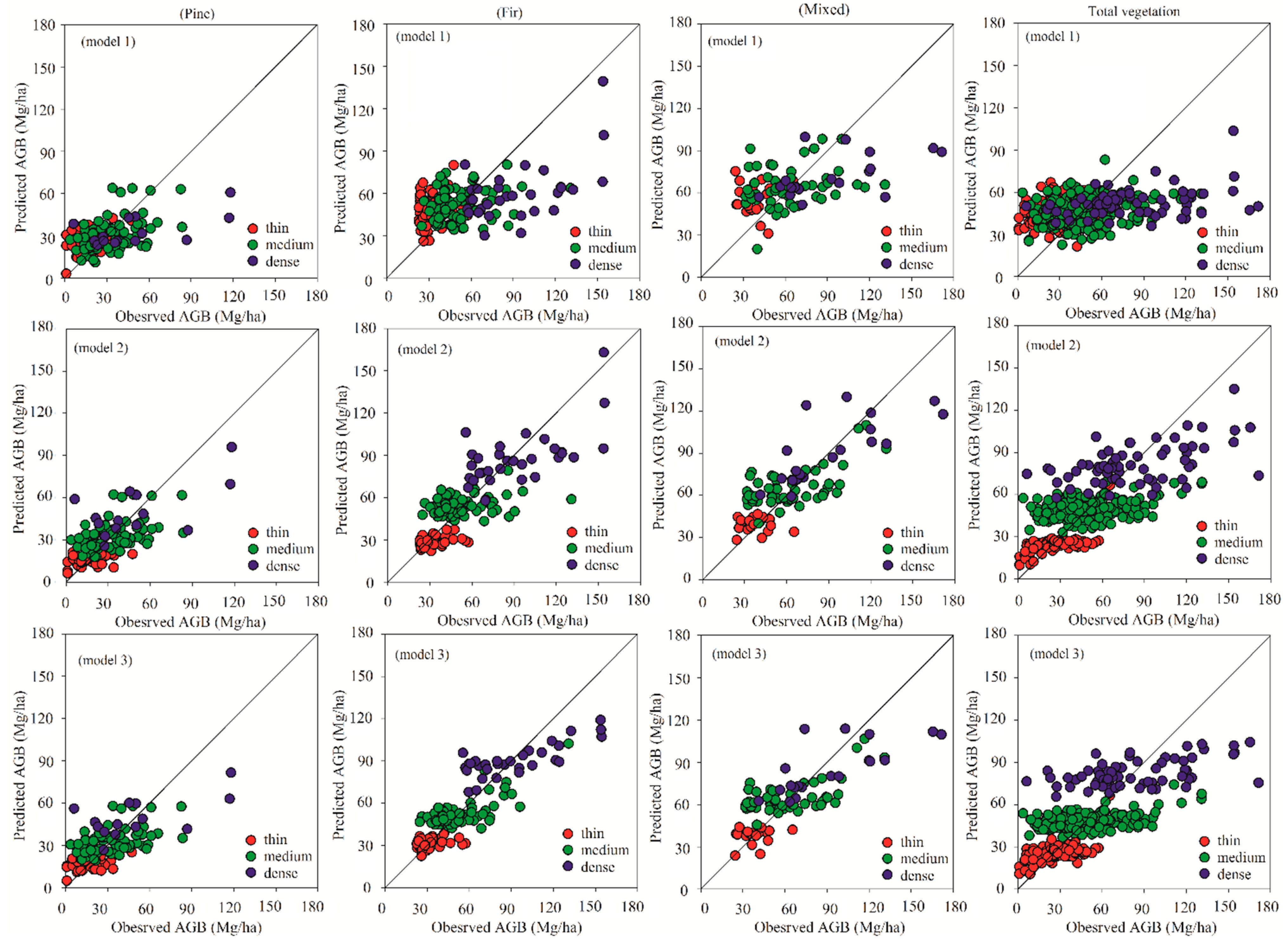
The performance of the predictions could be explained with the scatterplots showing the relationships between the predicted AGB values and observed AGB values (Figure 3). It indicates that the overestimation and underestimation problems were obvious for the linear model (model 1) for each vegetation type. This situation, especially, became worse for all the vegetation types in thin and dense plots. For model 2 and model 3, the overestimations and underestimations in thin and dense crown density plots were alleviated for four vegetation types, and the estimates were more accurate than model 1 (
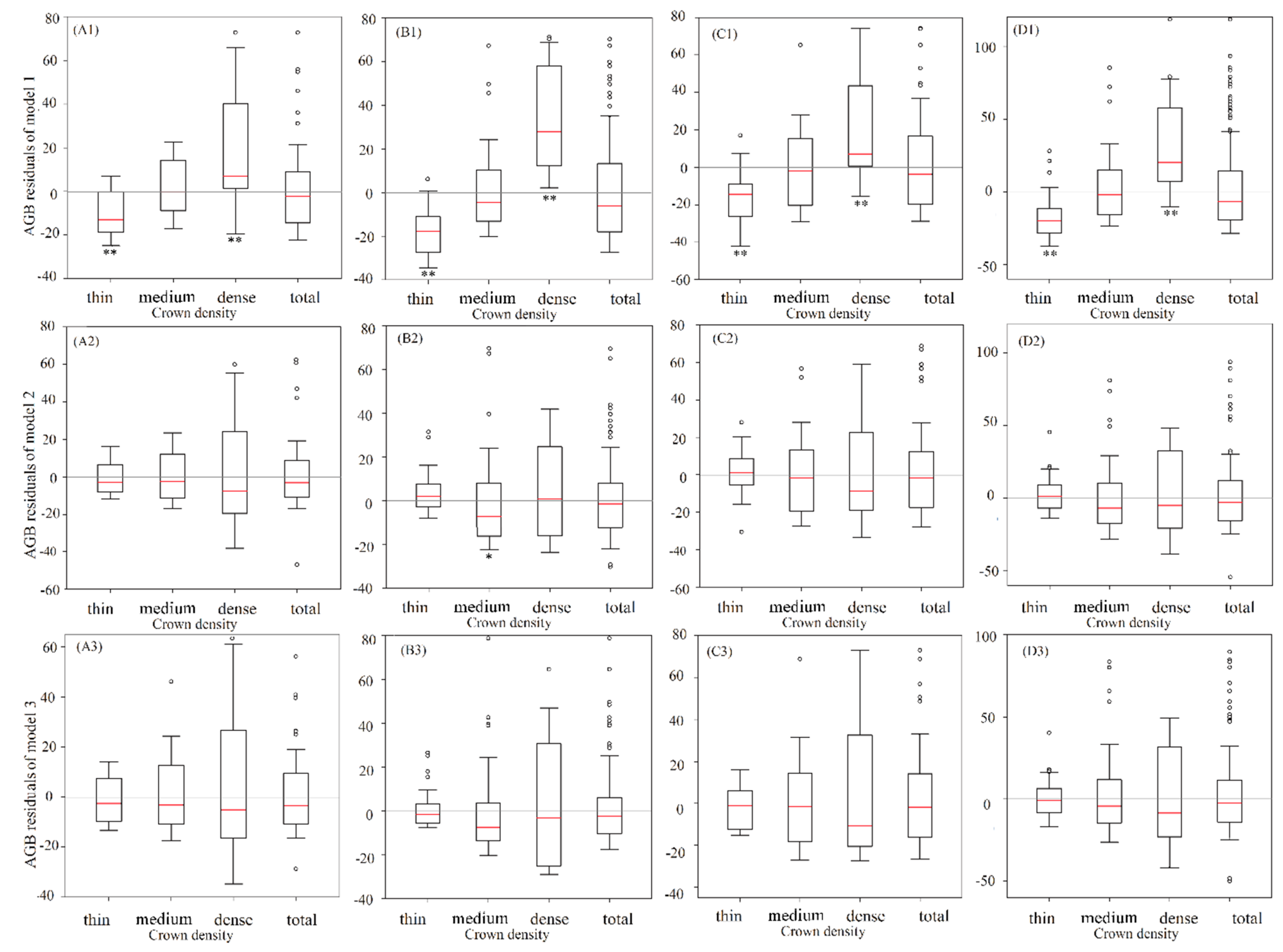
Figure 3). A single-sample t-test was used to compare the model residuals of models 1, 2, and 3 (Figure 4). In model 1, there were no significant differences between the residuals and 0 for the total plots and medium crown density plots for each vegetation type (Figure 4). In the thin crown density plots, the residual values of model 1 were significantly smaller than 0, and in the dense crown density plots, the residual values of model 1 were significantly larger than 0 (Figure 4). These results indicate that there were significant inaccuracies in the AGB estimations of the thin and dense plots of model 1 (the former was overestimated and the latter was underestimated) (Figure 4). The residuals of model 2 were significantly different from 0 only in the thin and medium crown density plots for the fir forest, whereas the other three vegetation types exhibited no significant differences in each crown density class. The residuals of model 3 were not significantly different from 0 for all vegetation types for the different crown density classes (Figure 4). The residual results indicate that model 2 and model 3 had higher accuracies of AGB estimation than model 1 for the different crown density classes.
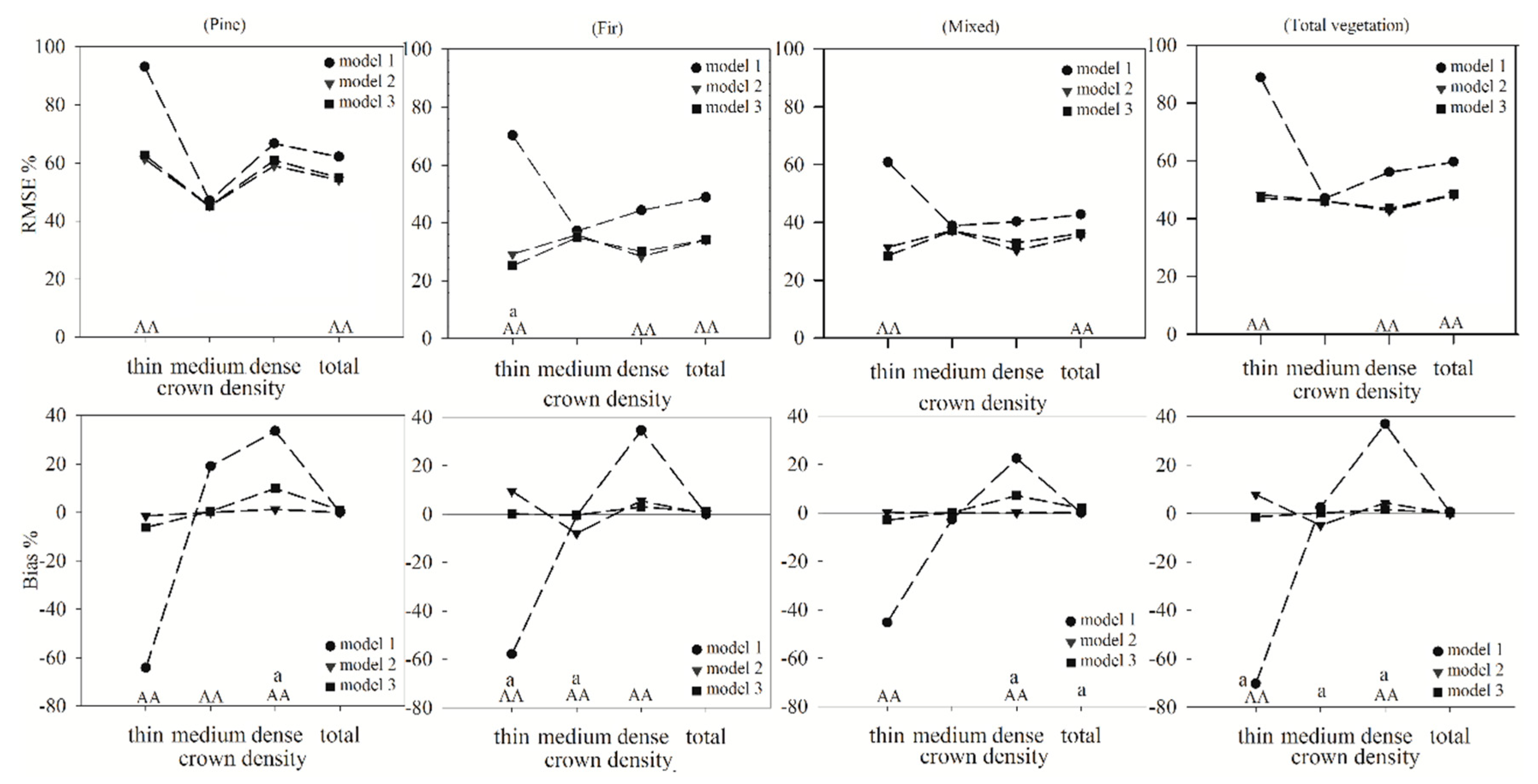
In this study, the RMSE% and Bias% of the three models of the different crown density classes were calculated for further comparison of the models (Figure 5). Generally, the RMSE% of model 2 and model 3 were lower than those of model 1 in the total plots for all vegetation types, and the differences in the RMSE% between model 1 and model 2 and between model 1 and model 3 were all significant. For the thin crown density plots, the differences in the RMSE% exceeded 27%, and both values were significantly different from the RMSE% of model 1. For the medium crown density plots, the RMSE% of model 2 and model 3 were smaller than those of model 1, but the differences between them were not significant. For the dense crown density plots, the differences in the RMSE% exceeded 5%, and the differences between model 2 and model 1 and between model 3 and model 1 were significant for the fir forest and total vegetation. In the thin and dense plots, the values of the Bias% for model 2 and model 3 were nearer to 0 than those of model 1, and the differences between model 2 and model 1 and between model 3 and model 1 were significant, indicating that model 2 and model 3 were more accurate than model 1 in these two crown density classes. In the medium crown density plots, the trends of the Bias% between model 1 and model 2 and between model 1 and model 3 were not clear, and significant decreases only existed in model 2 and model 3 of the pine forest. The total Bias% values were not significantly different between the three models for the different vegetation types, indicating that the overall estimated values obtained from models 1, 2, and 3 were not significantly different. The differences between model 2 and model 3 for the different vegetation types were compared. The overall RMSE% and Bias% values of model 2 and model 3 were not significantly different, and model 2 was slightly better than model 3, but the performances of model 2 and model 3 were different among the thin, medium, and dense crown density classes.

4. Discussion

The choice of the independent variables is important for remote-sensing-based AGB estimation models, and potential variables from the images, such as single bands, vegetation indices, transformed images, textural information were applied because of the correlation with forest biomass. The correlation analysis results of over 300 spectral variables and the AGB of different vegetation types indicated that only 30 spectral variables simultaneously had significant correlation with AGB. This indicated that a large amount of remote sensing information does not fully reflect the forest characteristics. During the modelling process, stepwise regression was used to select the independent variables that were closely related to AGB. Although this variable selection method depended on the degree of linear correlation, the variables with low correlation coefficients may have been selected and thus affected the accuracy of the model.
Linear stepwise regression models have been widely used for AGB estimation using remote sensing [7,23]. In this study, the R2 of the linear model (model 1) for the four vegetation types ranged from 0.1 to 0.3, indicating that the model had low accuracy. In addition, model 1 exhibited overestimation in the low crown density class and underestimation in the high crown density class of all vegetation types. The overestimations and underestimations of AGB were also investigated by Zhao et al., who determined that they were caused by the “global model (stepwise regression)” [40]. In addition, overestimations and underestimations have been observed when AGB was estimated using nonparametric models such as random forest, decision tree, and K-nearest neighbor methods [41,42,43]. In this study, the significant overestimations and underestimations of the linear model occurred in the thin (crown density < 0.4) and dense (crown density ≥ 0.7) plots, respectively. There were no significant overestimations or underestimations for model 2 and model 3 in the thin and dense plots. In addition, there were no significant differences between the linear dummy variable model (model 2) and linear mixed-effects model (model 3) except for the mixed forests (Table 8). However, in comparison with the model 1, model 2 and model 3 performed significantly better, and the results of the F-test and residuals verified the significant differences. The AGB estimation results of the three models were evaluated in the crown density classes and the results showed that the overestimation in the thin plots and underestimation in the dense plots of model 1 were not observed in model 2 and model 3.
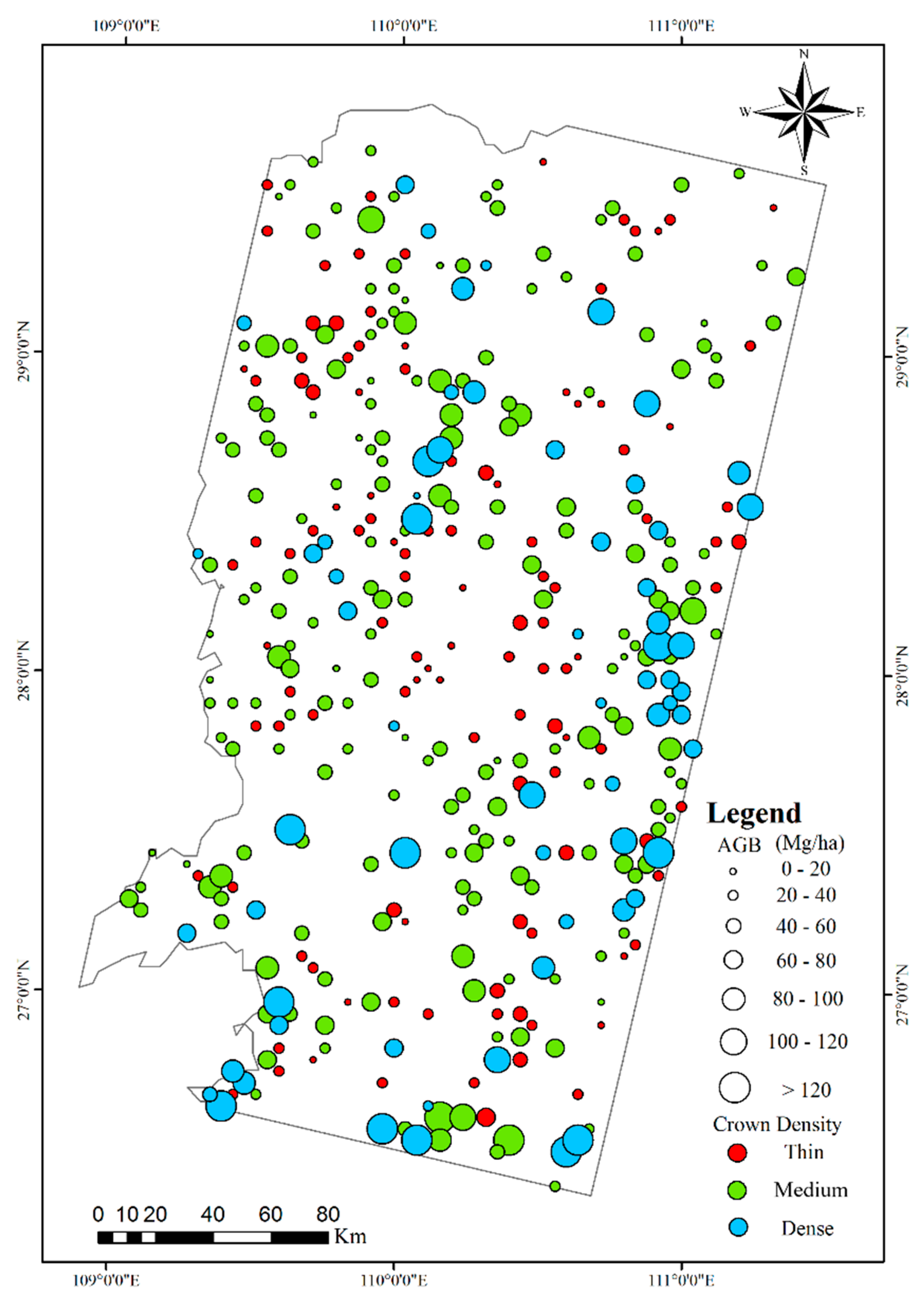
The average AGB estimates of the sample plots for the total vegetation in the “Greater Xiangxi” varied from 47.4 Mg/ha to 47.7 Mg/ha, which were very close to the referenced value (47.7 Mg/ha) of the plots measured, and the average AGB estimates of pine forest, fir forest, and mixed forest were also very close to those of the referenced values. In Hunan province, the average AGB value of pine forest in 2011 was 31.61 Mg/ha, and the average AGB value of fir forest in the forest average AGB values obtained from the sample plots of the 4th and 8th national forest inventories in 1990 and 2009 were 31.76 Mg/ha [44] and 27.56 Mg/ha, respectively. This implied that the AGB values of forests in the “Greater Xiangxi” were larger than those of the whole Hunan mainly because the study area was a key forestry area and had various protected forests.
A comparison of the R2adj and RMSE of the three models indicated that the performances of model 2 and model 3 were better than that of model 1. The dummy variable model considered the group differences as special fixed parameters. The purpose of using the dummy variable model in this study was to introduce the parameter of crown density class into the intercept of the model so that the degree of freedom of the error was increased and the variance of the error was decreased, thereby improving the precision of the model [45]. The linear mixed-effects model considered the group differences as two parts: One part was the difference caused by different groups, and the other was the difference caused by random effects. Since the error and the random effect of the variance-covariance structures was considered, the model had high precision. Some studies compared dummy variable models with mixed-effects models for the estimation of large-scale forest growth models and the determination of biomass allometric growth equations. The linear mixed-effects model was a compromise between the dummy variable model and the linear model; in most cases, the dummy variable model was slightly better than the mixed-effects model, but this often depended on the sample size [45,46]. In this study, the sample plots were divided into the three categories of thin, medium, and dense crown density. The overall RMSE% and Bias% of model 2 were better than model 3, which supported the aforementioned results. In the past, the application of dummy variable models and mixed-effects models focused on the determination of allometric growth equations, whereas in this study, we considered whether the partition of the crown density classes improved the estimation accuracy of AGB using remote sensing data.
In statistics and biometrics, it is often debated whether the dummy variable model or mixed-effects model should be selected [46]. The choice often depends on the number of groups (random effects/dummy variables, crown density classes in this study) and the number of samples in each group. For a small group size (less than 10), the dummy variable model is commonly preferred; otherwise, the mixed-effects model is more appropriate [37,47]. Unlike in most other studies, we not only compared the overall differences between the linear dummy variable model and linear mixed-effects model but also the differences in model performance among different groups. Although the overall RMSE% and Bias% were better in model 2 than in model 3, this trend was not always the same for the different crown density classes. In the fir forest and the total vegetation, groups that had a large number of samples, the RMSE% and Bias% were smaller for model 3 than model 2 for all crown density classes. In pine and mixed forests, which had a small number of samples in each group, the RMSE% and Bias% were smaller for model 2 than model 3 for all crown density classes. Therefore, regardless of which of the models was chosen, we believe that if the overall differences between the two models are not significant, the fitting effects of the groups should be compared and the model with good performance in each group should be selected.
The climate of this region is a typical subtropical monsoon humid climate, and the typical forests are evergreen broad leaf forests and evergreen coniferous forests. In this study, the mixed forests were almost evergreen coniferous forests, and the seasonal variation of the vegetation types were not obvious. Many studies analyzed the variation of different vegetation types (NDVI) in the subtropical regions of China. They demonstrated that the NDVI of evergreen forests (evergreen broad leaf forest and evergreen coniferous forest) had no obviously seasonal variation [48]. Besides, the seasonal variations of leaf area index (LAI) and clumping index (CI) were very small because the canopy structure of evergreen forests were stable through the year [49,50], and texture information which referred the forest structure were relatively stable in the imagery. The spectral characteristics of remote sensing images are influenced by the soil, topography, vegetation type, forest structure, and other factors. It is important to choose appropriate spectral variables as independent variables in AGB estimation using remote-sensing-based methods [5,51]. Many studies have shown that when only spectral indices were used in AGB estimation, saturation occurred and caused inaccuracies of AGB estimation. Texture information calculated from a small neighborhood of pixels [26] may have a stronger correlation with AGB than spectral indices, and in some regions, AGB may only be closely correlated with texture information rather than spectral information. Texture information has been demonstrated to be an important factor in remote-sensing-based AGB estimation [52,53].
The independent variables of the linear model in this study illustrated that texture information had considerable influences on the accuracy of the AGB estimation in our study area. The linear models had low accuracy for the thin and dense crown density classes, and the linear dummy variable models and linear mixed-effects models had higher accuracy because the crown density classes were considered. The results indicate that the crown density class may be an important factor affecting the accuracy of AGB estimation. The sensitivity to the stand information decreased with increasing crown density in the dense stands; the spectral information may be affected by other non-forest characteristics in thin stands with low AGB, causing the low accuracy of the AGB estimation model. Many studies have demonstrated that a complex stand structure and high crown density caused saturation in remote sensing images and low crown density and sparse trees increased the occurrence of soil/vegetation mixed pixels [6,54,55]. The saturation and mixed pixels problems have attracted increased attention for remote-sensing-based AGB estimation. In this study, we demonstrated that the crown density classes influenced the accuracy of AGB estimation; however, the underlying mechanisms and relationships should be studied in more detail in the future.
In this study, the models for AGB estimation were explored combining sample plot data and remote sensing, and the results illustrated that the crown density was a factor that influences model accuracy. The crown density data incorporated in the linear dummy variable model and linear mixed-effects model were the most accurate. The aim of this study was to demonstrate that the crown density is an important factor that influences the accuracy of the models. A large amount of research has explored the potential of using satellite imagery for exploring remote-sensing-based methods of crown density, and there are more precise results [56]. This should be examined in future research for mapping large-scale AGB using our models when the crown density data were not available.

5. Conclusions

Permanent sample plot data of AGB of evergreen forests and Landsat 8 OLI images in the subtropical region of western Hunan province were used to develop remote-sensing-based AGB estimation models. The linear model, linear dummy variable model, and linear mixed-effects model were used to determine if the accuracy of the AGB linear estimation model could be improved by considering crown density classes. The forest AGB in our study exhibited significant differences between the thin, medium, and dense crown density classes for each vegetation type, and the AGB increased with increasing crown density. The results of the models indicate that the performance of the linear model was affected to a large extent by the crown density classes, resulting in the low accuracy of the linear model. The model-fitting results of the linear dummy variable models and linear mixed-effects models, which considered the crown density classes, were better than those of the linear models. The accuracy of the AGB estimation was significantly higher for the linear dummy variable models and linear mixed-effects models than the linear models, especially in the thin and dense crown density classes. There were no significant differences in the overall estimation accuracy between linear dummy models and linear mixed-effects models, but there were significant differences in some crown density classes of different vegetation types. The choice between the linear dummy variable model or linear mixed-effects model depended on the number of groups and sample size of the groups; when the sample size was large enough, each of the models met the accuracy requirements for AGB estimation.

Author Contributions

C.L. and M.L. conceived and designed the experiments. C.L. and Y.L. performed the experiments and analyzed the data. C.L. and M.L. wrote the paper.

Funding

This research was supported by the Doctorate Fellowship Foundation of Nanjing Forestry University and National Natural Science Foundation (NO. 31770679).

Acknowledgments

We would like to thank the Top-notch Academic Programs Project of Jiangsu Higher Education Institutions, China (TAPP, PPZY2015A062).

Conflicts of Interest

The authors declare no conflict of interest.

References

  1. West, P.W. Tree and Forest Measurement, 2nd ed.; Springer: Berlin, Germany, 2009; ISBN 9783540959656. [Google Scholar]
  2. Lieth, H.; Whittaker, R.H. Primary Productivity of the Biosphere; Springer-Verlag: Berlin, Germany, 1975; Volume 14, ISBN 978-3-642-80915-6. [Google Scholar]
  3. Tian, X.; Li, Z.; Su, Z.; Chen, E.; van der Tol, C.; Li, X.; Guo, Y.; Li, L.; Ling, F. Estimating montane forest above-ground biomass in the upper reaches of the Heihe River Basin using Landsat-TM data. Int. J. Remote Sens. 2014, 35, 7339–7362. [Google Scholar] [CrossRef]
  4. Ketterings, Q.M.; Coe, R.; van Noordwijk, M.; Ambagau, Y.; Palm, C.A. Reducing uncertainty in the use of allometric biomass equations for predicting above-ground tree biomass in mixed secondary forests. For. Ecol. Manag. 2001, 146, 199–209. [Google Scholar] [CrossRef]
  5. Lu, D.; Chen, Q.; Wang, G.; Liu, L.; Li, G.; Moran, E. A survey of remote sensing-based aboveground biomass estimation methods in forest ecosystems. Int. J. Digit. Earth 2016, 9, 63–105. [Google Scholar] [CrossRef]
  6. Safari, A.; Sohrabi, H.; Powell, S.; Shataee, S. A comparative assessment of multi-temporal Landsat 8 and machine learning algorithms for estimating aboveground carbon stock in coppice oak forests. Int. J. Remote Sens. 2017, 38, 6407–6432. [Google Scholar] [CrossRef]
  7. Lu, D. Review Article The potential and challenge of remote sensing-based biomass estimation. Int. J. Remote Sens. 2006, 27, 1297–1328. [Google Scholar] [CrossRef]
  8. Sun, H.; Qie, G.; Wang, G.; Tan, Y.; Li, J.; Peng, Y.; Ma, Z.; Luo, C. Increasing the accuracy of mapping urban forest carbon density by combining spatial modeling and spectral unmixing analysis. Remote Sens. 2015, 7, 15114–15139. [Google Scholar] [CrossRef]
  9. Galidaki, G.; Zianis, D.; Gitas, I.; Radoglou, K.; Karathanassi, V.; Tsakiri–Strati, M.; Woodhouse, I.; Mallinis, G. Vegetation biomass estimation with remote sensing: Focus on forest and other wooded land over the Mediterranean ecosystem. Int. J. Remote Sens. 2017, 38, 1940–1966. [Google Scholar] [CrossRef]
  10. Mitchard, E.T.A.; Saatchi, S.S.; Woodhouse, I.H.; Nangendo, G.; Ribeiro, N.S.; Williams, M.; Ryan, C.M.; Lewis, S.L.; Feldpausch, T.R.; Meir, P. Using satellite radar backscatter to predict above-ground woody biomass: A consistent relationship across four different African landscapes. Geophys. Res. Lett. 2009, 36. [Google Scholar] [CrossRef] [Green Version]
  11. Sun, G.; Ranson, K.J.; Guo, Z.; Zhang, Z.; Montesano, P.; Kimes, D. Forest biomass mapping from lidar and radar synergies. Remote Sens. Environ. 2011, 115, 2906–2916. [Google Scholar] [CrossRef] [Green Version]
  12. Qazi, W.A.; Baig, S.; Gilani, H.; Waqar, M.M.; Dhakal, A.; Ammar, A. Comparison of forest aboveground biomass estimates from passive and active remote sensing sensors over Kayar Khola watershed, Chitwan district, Nepal. J. Appl. Remote Sens. 2017, 11, 026038. [Google Scholar] [CrossRef]
  13. Timothy, D.; Onisimo, M.; Cletah, S.; Adelabu, S.; Tsitsi, B. Remote sensing of aboveground forest biomass: A review. Trop. Ecol. 2016, 57, 125–132. [Google Scholar]
  14. Zhu, C.; Lu, D.; Victoria, D.; Dutra, L.V. Mapping fractional cropland distribution in Mato Grosso, Brazil using time series MODIS enhanced vegetation index and Landsat Thematic Mapper data. Remote Sens. 2016, 8, 22. [Google Scholar] [CrossRef]
  15. Zhu, X.; Liu, D. Improving forest aboveground biomass estimation using seasonal Landsat NDVI time-series. ISPRS J. Photogramm. Remote Sens. 2015. [Google Scholar] [CrossRef]
  16. Asner, G. Biophysical and Biochemical Sources of Variability in Canopy Reflectance. Remote Sens. Environ. 1998, 64, 234–253. [Google Scholar] [CrossRef]
  17. Ollinger, S.V. Sources of Variability in Canopy Reflectance and the Convergent Properties of Plants. New Phytol. 2011, 189, 375–394. [Google Scholar] [CrossRef] [PubMed]
  18. Ruimy, A.; Saugier, B.; Dedieu, G. Methodology for the estimation of terrestrial net primary production from remotely sensed data. J. Geophys. Res. 1994, 99, 5263–5283. [Google Scholar] [CrossRef]
  19. Fensholt, R.; Sandholt, I.; Rasmussen, M.S.; Stisen, S.; Diouf, A. Evaluation of satellite based primary production modelling in the semi-arid Sahel. Remote Sens. Environ. 2006, 105, 173–188. [Google Scholar] [CrossRef]
  20. Asner, G.P.; Levick, S.R.; Smit, I.P.J. Remote sensing of fractional cover and biochemistry in Savannas. In Ecosystem Function in Savannas: Measurement and Modeling at Landscape to Global Scales; CRC Press: Boca Raton, FL, USA, 2010; ISBN 9781439804711. [Google Scholar]
  21. Kumar, L.; Sinha, P.; Taylor, S.; Alqurashi, A.F. Review of the use of remote sensing for biomass estimation to support renewable energy generation. J. Appl. Remote Sens. 2015, 9, 097696. [Google Scholar] [CrossRef]
  22. Foody, G.M.; Boyd, D.S.; Cutler, M.E.J. Predictive relations of tropical forest biomass from Landsat TM data and their transferability between regions. Remote Sens. Environ. 2003, 85, 463–474. [Google Scholar] [CrossRef]
  23. Lu, D.; Chen, Q.; Wang, G.; Moran, E.; Batistella, M.; Zhang, M.; Vaglio Laurin, G.; Saah, D. Aboveground Forest Biomass Estimation with Landsat and LiDAR Data and Uncertainty Analysis of the Estimates. Int. J. For. Res. 2012, 2012, 1–16. [Google Scholar] [CrossRef] [Green Version]
  24. Lu, D.; Batistella, M. Exploring TM image texture and its relationships with biomass estimation in Rondônia, Brazilian Amazon. Acta Amaz. 2005, 35, 249–257. [Google Scholar] [CrossRef]
  25. Powell, S.L.; Cohen, W.B.; Healey, S.P.; Kennedy, R.E.; Moisen, G.G.; Pierce, K.B.; Ohmann, J.L. Quantification of live aboveground forest biomass dynamics with Landsat time-series and field inventory data: A comparison of empirical modeling approaches. Remote Sens. Environ. J. 2010, 114, 1053–1068. [Google Scholar] [CrossRef]
  26. Kelsey, K.C.; Neff, J.C. Estimates of aboveground biomass from texture analysis of landsat imagery. Remote Sens. 2014, 6, 6407–6422. [Google Scholar] [CrossRef]
  27. Wang, G.; Zhang, M.; Gertner, G.Z.; Oyana, T.; McRoberts, R.E.; Ge, H. Uncertainties of mapping aboveground forest carbon due to plot locations using national forest inventory plot and remotely sensed data. Scand. J. For. Res. 2011, 26, 360–373. [Google Scholar] [CrossRef]
  28. Fehrmann, L.; Lehtonen, A.; Kleinn, C.; Tomppo, E. Comparison of linear and mixed-effect regression models and a k-nearest neighbour approach for estimation of single-tree biomass. Can. J. For. Res. 2008, 38, 1–9. [Google Scholar] [CrossRef]
  29. Yang, X.; Xue, S. Geographic Features of Forestry Resource in Hunan. Econ. Geogr. 2001, 21, 736–739. (In Chinese) [Google Scholar]
  30. Xu, M.; Liu, C. Connotation and Evaluation of Regional Economic Transition Degree—A Case Study of the Western Hunan Area. J. Nat. Resour. 2015, 30, 1675–1685. (In Chinese) [Google Scholar]
  31. Fang, J.; Chen, A.; Peng, C.; Zhao, S.; Ci, L. Changes in forest biomass carbon storage in China between 1949 and 1998. Science 2001, 292, 2320–2322. [Google Scholar] [CrossRef]
  32. Zhang, M.; Wang, G. The forest biomass dynamics of Zhejiang Province. Acta Ecol. Sin. 2008, 28, 5665–5674. (In Chinese) [Google Scholar]
  33. Chander, G.; Markham, B.L.; Helder, D.L. Summary of current radiometric calibration coefficients for Landsat MSS, TM, ETM+, and EO-1 ALI sensors. Remote Sens. Environ. 2009, 113, 893–903. [Google Scholar] [CrossRef] [Green Version]
  34. Hantson, S.; Chuvieco, E. Evaluation of different topographic correction methods for landsat imagery. Int. J. Appl. Earth Obs. Geoinf. 2011, 13, 691–700. [Google Scholar] [CrossRef]
  35. Boyd, D.S.; Foody, G.M.; Ripple, W.J. Evaluation of approaches for forest cover estimation in the Pacific Northwest, USA, using remote sensing. Appl. Geogr. 2002, 22, 375–392. [Google Scholar] [CrossRef]
  36. Tang, S.Z.; Li, Y. Statistical Foundation for Biomathematical Models; Science Press: Beijing, China, 2002. (In Chinese) [Google Scholar]
  37. Fu, L.Y.; Zeng, W.S.; Tang, S.Z.; Sharma, R.P.; Li, H.K. Using linear mixed model and dummy variable model approaches to construct compatible single-tree biomass equations at different scales—A case study for Masson pine in Southern China. J. For. Sci. 2012, 58, 101–115. [Google Scholar] [CrossRef]
  38. Pinheiro, J.; Bates, D. Mixed-Effects Models in S and S-PLUS; Springer-Verlag: New York, NY, USA, 2000; ISBN 9780387989570. [Google Scholar]
  39. Fang, Z.; Bailey, R.L. Nonlinear mixed effects modeling for slash pine dominant height growth following intensive silvicultural treatments. For. Sci. 2001, 47, 287–300. [Google Scholar]
  40. Zhao, P.; Lu, D.; Wang, G.; Wu, C.; Huang, Y.; Yu, S. Examining spectral reflectance saturation in landsat imagery and corresponding solutions to improve forest aboveground biomass estimation. Remote Sens. 2016, 8, 469. [Google Scholar] [CrossRef]
  41. Reese, H.; Nilsson, M.; Sandström, P.; Olsson, H. Applications using estimates of forest parameters derived from satellite and forest inventory data. Comput. Electron. Agric. 2002, 37, 37–55. [Google Scholar] [CrossRef] [Green Version]
  42. Blackard, J.A.; Finco, M.V.; Helmer, E.H.; Holden, G.R.; Hoppus, M.L.; Jacobs, D.M.; Lister, A.J.; Moisen, G.G.; Nelson, M.D.; Riemann, R.; et al. Mapping U.S. forest biomass using nationwide forest inventory data and moderate resolution information. Remote Sens. Environ. 2008, 112, 1658–1677. [Google Scholar] [CrossRef]
  43. Main-Knorn, M.; Moisen, G.G.; Healey, S.P.; Keeton, W.S.; Freeman, E.A.; Hostert, P. Evaluating the remote sensing and inventory-based estimation of biomass in the western carpathians. Remote Sens. 2011, 3, 1427–1446. [Google Scholar] [CrossRef]
  44. Jiao, X.M.; Xiang, W.H.; Tian, D.L. Carbon Storage of Forest Vegetation and Its Geographical Distribution in Hunan Province. J. Cent. South For. Univ. 2005, 25, 4–8. (In Chinese) [Google Scholar]
  45. Zeng, W.S.; Zhang, H.R.; Tang, S.Z. Using the dummy variable model approach to construct compatible single-tree biomass equations at different scales—A case study for Masson pine (Pinus massoniana) in southern China. Can. J. For. Res. 2011, 41, 1547–1554. [Google Scholar] [CrossRef]
  46. Wang, M.; Borders, B.E.; Zhao, D. An empirical comparison of two subject-specific approaches to dominant heights modeling: The dummy variable method and the mixed model method. For. Ecol. Manag. 2008, 255, 2659–2669. [Google Scholar] [CrossRef]
  47. Chen, D.; Huang, X.; Zhang, S.; Sun, X. Biomass modeling of larch (Larix spp.) plantations in China based on the mixed model, dummy variable model, and Bayesian hierarchical model. Forests 2017, 8, 268. [Google Scholar] [CrossRef]
  48. Wang, Q.; Li, J. Seasonal variation of evergreen land coverage in poyang lake watershed using multi-temporal spot4-vegetation data. Resour. Environ. Yangtze Basin 2008, 17, 866–871. (In Chinese) [Google Scholar]
  49. Gaolong, Z. Spatial-temporal characteristics of foliage clumping index in China during 2000–2013. Chin. Sci. Bull. 2016, 61, 1595–1603. (In Chinese) [Google Scholar] [CrossRef]
  50. Liu, Y.B.; Ju, W.M.; Chen, J.M.; Zhu, G.L.; Xing, B.L.; Zhu, J.F.; He, M.Z. Spatial and temporal variations of forest LAI in China during 2000–2010. Chin. Sci. Bull. 2012, 57, 2846–2856. (In Chinese) [Google Scholar] [CrossRef] [Green Version]
  51. Zhao, P.; Lu, D.; Wang, G.; Liu, L.; Li, D.; Zhu, J.; Yu, S. Forest aboveground biomass estimation in Zhejiang Province using the integration of Landsat TM and ALOS PALSAR data. Int. J. Appl. Earth Obs. Geoinf. 2016, 53, 1–15. [Google Scholar] [CrossRef]
  52. Lu, D. Aboveground biomass estimation using Landsat TM data in the Brazilian Amazon. Int. J. Remote Sens. 2005, 26, 2509–2525. [Google Scholar] [CrossRef]
  53. Eckert, S. Improved forest biomass and carbon estimations using texture measures from worldView-2 satellite data. Remote Sens. 2012, 4, 810–829. [Google Scholar] [CrossRef]
  54. Du, H.; Cui, R.; Zhou, G.; Shi, Y.; Xu, X.; Fan, W.; Lü, Y. The responses of Moso bamboo (Phyllostachys heterocycla var. pubescens) forest aboveground biomass to Landsat TM spectral reflectance and NDVI. Acta Ecol. Sin. 2010, 30, 257–263. [Google Scholar] [CrossRef]
  55. Wu, C.; Shen, H.; Wang, K.; Shen, A.; Deng, J.; Gan, M. Landsat imagery-based above ground biomass estimation and change investigation related to human activities. Sustainibility 2016, 8, 159. [Google Scholar] [CrossRef]
  56. Karlson, M.; Ostwald, M.; Reese, H.; Sanou, J.; Tankoano, B.; Mattsson, E. Mapping tree canopy cover and aboveground biomass in Sudano-Sahelian woodlands using Landsat 8 and random forest. Remote Sens. 2015, 7, 10017–10041. [Google Scholar] [CrossRef]
Figure 1. The location of study area: (a) The study area location in China; (b) the western Hunan in Hunan province; and (c) a false color composite of Landsat 8 OLI band 6 in red, band 5 in green, and band 4 in blue.
Forests 10 00104 g001
Figure 2. Spatial distribution of sampling plots corresponding to plots of aboveground biomass (AGB) values and crown density class across the western Hunan.
Forests 10 00104 g002
Figure 3. The relationships between predicted AGB from different models in different crown density against observed AGB for different vegetation types.
Forests 10 00104 g003
Figure 4. Residual boxplots of AGB of model 1, model 2, and model 3 for different vegetation types among different crown density classes: (AD) represents pine forest, fir forest, mixed forest, and total vegetation, respectively (model 1—linear regression model; model 2—linear dummy variable model; model 3—linear mixed-effects model; ** indicates that the residuals were significantly different from 0 at the 0.01 level; * indicates that the residuals were significantly different from 0 at the 0.05 level).
Forests 10 00104 g004
Figure 5. Comparison of root mean square error percent (RMSE%) and Bias percent (Bias%) results at different crown density classes of models 1–3 for pine forest, fir forest, mixed forest, and total vegetation. The significant differences between model 1 and model 2, and model 1 and model 3 for RMSE% and Bias% are expressed in capital letters (AA), and the lowercase letter (a) represents significant differences between model 2 and model 3.
Forests 10 00104 g005
Table 1. The basic statistics of the sample plots by crown density classes and vegetation types.
Vegetation TypeCrown DensityAGB (Mg/ha)
No.MinimumMeanMaximumStandard Deviation
PineThin411.0516.4047.3310.61
Middle703.6133.6083.5817.06
Dense146.1651.17118.0735.57
Total1251.0529.65118.0720.94
FirThin5422.7631.1157.468.70
Middle7724.7251.18130.8718.37
Dense3155.5592.55154.4830.65
Total16222.7652.41154.4828.68
MixedThin1824.5237.7065.4210.53
Middle5331.7462.13131.0324.02
Dense1941.2892.57171.5337.06
Total9024.5663.67171.5330.86
TotalThin1131.0526.6565.4212.77
Middle2003.6148.11131.0322.68
Dense646.1683.26171.5337.39
Total3771.0547.70171.5330.06
Table 2. Spectral variables derived from a total of seven bands for the Landsat 8 OLI image.
Spectral VariablesDefinitions of Spectral VariablesNo.
Original Bandb1—coastal, b2—blue, b3—green (GRN), b4—red (RED), b5—near infrared (NIR), b6—shortwave infrared1 (SWIR1), b7—shortwave infrared2 (SWIR2)7
Inversions of bandi I B i = 1 / b i , i = 1,…,77
Simple two-band ratios ( S R i , j ) S R i , j = b i / b j , i, j = 1,…7; ij42
Three-band ratios S R i , j , k = b i / ( b j + b k ) , i, j, k = 1,…,7; ijk, j < k106
Vegetation indicesNormalized difference vegetation index (NDVI), atmospherically resistant vegetation index (ARVI), soil adjusted vegetation index ( SAVI l =   ( b 5 b 4 ) ( 1 + l ) / ( b 5 + b 4 + l ) , l = 0.1), atmospherically resistant vegetation index (ARVI), enhance vegetation index (EVI), albedo, sum of three visible bands ( V I S 234 , V I S 234 = b 2 + b 3 + b 4 )7
Principal component analysisThe first 3 PCs from principal component analysis (PCA1, PCA2, PCA3)3
Texture measuresGrey-level co-occurrence matrix-based texture measures of original bands ( b i ), including contrast ( b i C O N j ), correlation ( b i C O R j ), dissimilarity ( b i D I S j ), entropy ( b i E N j ), homogeneity ( b i H O j ), angular second moment ( b i S E M j ), mean ( b i M E j ), and variance( b i V A j ) with different window sizes j (3 × 3, 5 × 5, 7 × 7)168
Table 3. Pearson correlation coefficients between remote sensing factors and aboveground biomass (AGB).
VariablesCorrelation CoefficientsVariablesCorrelation CoefficientsVariablesCorrelation CoefficientsVariablesCorrelation Coefficients
b3−0.254 ** S R 37 −0.236 ** S R 416 −0.210 ** b 4 M E 5 −0.276 **
b4−0.233 ** S R 46 −0.207 ** S R 417 −0.215 ** b 7 C O R 7 0.258 **
V I S 234 −0.260 ** S R 47 −0.227 ** S R 426 −0.206 ** b 3 M E 7 −0.251 **
ARVI0.162 * S R 64 0.227 ** b 3 M E 3 −0.265 ** b 4 M E 7 −0.242 **
I B 4 0.247 ** S R 73 0.236 ** b 4 M E 3 −0.247 ** b 2 S E M 5 0.251 **
I B 2 0.232 ** S R 124 0.210 ** b 5 V A 3 0.272 ** b 2 S E M 7 0.230 **
S R 14 0.228 ** S R 134 0.204 * b 2 C O R 5 0.260 **————
S R 41 −0.244 * S R 327 −0.229 ** b 3 M E 5 −0.279 **————
* Indicates a significance level of 0.05 and ** a significance level of 0.01.
Table 4. Parameter estimates of the linear model (model 1).
Vegetation TypeParameterEstimateStd.coefp-ValueVegetation TypeParameterEstimateStd.coefp-Value
Pine b 2 C O R 5 24.140.33<0.01Fir b 5 V A 3 1.140.25<0.01
S R 327 −165.54−0.27<0.01 I B 2 1061.000.61<0.01
b 2 S E M 5 19.470.17<0.01 b 2 S E M 7 36.490.24<0.01
b 3 M E 5 6.900.40<0.01
Mixed b 7 C O R 7 30.550.30<0.01Total vegetation b 3 M E 7 −3.62−0.25<0.01
b 4 M E 7 −10.05−0.60<0.01 b 5 V A 3 0.830.14<0.01
V I S 234 9.000.36<0.01 b 2 S E M 5 15.360.09<0.05
Table 5. Parameter estimates of the linear dummy variable model (model 2) and linear mixed-effects model (model 3).
Vegetation TypeModel 2Vegetation TypeModel 3
ParameterEstimateS.D.p-ValueParameterEstimateS.D.p-Value
Pine b 2 C O R 5 16.704.77<0.01Pine b 2 C O R 5 13.353.77<0.01
S R 327 −113.5248.43<0.05 S R 327 −118.0021.87<0.01
b 2 S E M 5 16.856.86<0.05 b 2 S E M 5 12.676.15<0.05
Fir b 5 V A 3 0.620.22<0.01Fir b 5 V A 3 0.160.20<0.05
I B 2 732.08208.43<0.01 I B 2 515.01172.84<0.01
b 2 S E M 7 17.187.68<0.05 b 2 S E M 7 5.746.06<0.05
b 3 M E 5 5.292.08<0.01 b 3 M E 5 4.441.69<0.01
Mixed b 7 C O R 7 23.657.636<0.01Mixed b 7 C O R 7 10.556.79<0.05
b 4 M E 7 −4.803.665<0.05 b 4 M E 7 −1.422.86<0.05
V I S 234 6.285.165<0.05 V I S 234 0.744.09<0.05
Total vegetation b 3 M E 7 −2.200.66<0.01Total vegetation b 3 M E 7 −1.600.50<0.01
b 5 V A 3 0.480.21<0.05 b 5 V A 3 0.250.20<0.05
b 2 S E M 5 8.055.49<0.05 b 2 S E M 5 1.074.56<0.05
Table 6. The model fitting results of model 1 for different vegetation types.
Vegetation TypeR2R2adjRMSEPredict Mean
Pine0.230.2118.4129.64
Fir0.220.2225.5752.43
Mixed0.210.1927.2863.67
Total vegetation0.110.1028.4747.40
Table 7. The model fitting results of model 2 (linear dummy variable model) and model 3 (linear mixed-effects model) for different vegetation types.
Vegetation TypeModel#R2R2adjRMSEPredict Mean
Pine20.410.4016.0529.65
30.390.3816.2929.36
Fir20.610.6117.8852.39
30.610.6117.9251.95
Mixed20.460.4422.5663.64
30.430.4223.1262.41
Total vegetation20.410.4122.9947.70
30.410.4123.0747.51
Table 8. The comparisons of linear models (model 1), linear dummy variable models (model 2), and linear mixed-effects models (model 3). p-Value is from the F-test used to compare the similarity of models 1–3 against the null hypothesis of no significant difference.
Vegetation TypeModel#Models 1–3Model 2 and Model 3
F-Valuep-ValueF-Valuep-Value
Pine1
211.76<0.01
34.12<0.052.440.12
Fir1
229.58<0.01
317.31<0.011.280.26
Mixed1
29.37<0.01
30.770.384.690.03
Total vegetation1
2111.48<0.01
366.03<0.012.950.09

