Article

Lidar-Derived Tree Crown Parameters: Are They New Variables Explaining Local Birch (Betula sp.) Pollen Concentrations?

1
Laboratory of Biological Spatial Information, Faculty of Biology, Adam Mickiewicz University, Uniwersytetu Poznańskiego 6, 61–614 Poznań, Poland
2
Laboratory of Aeropalynology, Faculty of Biology, Adam Mickiewicz University, Uniwersytetu Poznańskiego 6, 61–614 Poznań, Poland
3
Students Nature Association, Faculty of Biology, Adam Mickiewicz University, Uniwersytetu Poznańskiego 6, 61–614 Poznań, Poland
4
Department of Plant Taxonomy, Faculty of Biology, Adam Mickiewicz University, Uniwersytetu Poznańskiego 6, 61–614 Poznań, Poland
*
Author to whom correspondence should be addressed.
Forests 2019, 10(12), 1154; https://doi.org/10.3390/f10121154
Submission received: 30 September 2019 / Revised: 10 December 2019 / Accepted: 13 December 2019 / Published: 17 December 2019
(This article belongs to the Special Issue Study of Tree Pollen and Pollination)

Abstract

:
Birch trees are abundant in central and northern Europe and are dominant trees in broadleaved forests. Birches are pioneer trees that produce large quantities of allergenic pollen efficiently dispersed by wind. The pollen load level depends on the sizes and locations of pollen sources, which are important for pollen forecasting models; however, very limited work has been done on this topic in comparison to research on anthropogenic air pollutants. Therefore, we used highly accurate aerial laser scanning (Light Detection and Ranging—LiDAR) data to estimate the size and location of birch pollen sources in 3-dimensional space and to determine their influence on the pollen concentration in Poznań, Poland. LiDAR data were acquired in May 2012. LiDAR point clouds were clipped to birch individuals (mapped in 2012–2014 and in 2019), normalised, filtered, and individual tree crowns higher than 5 m were delineated. Then, the crown surface and volume were calculated and aggregated according to wind direction up to 2 km from the pollen trap. Consistent with LIDAR data, hourly airborne pollen measurements (performed using a Hirst-type, 7-day volumetric trap), wind speed and direction data were obtained in April 2012. We delineated 18,740 birch trees, with an average density of 14.9/0.01 km2, in the study area. The total birch crown surface in the 500–1500 m buffer from the pollen trap was significantly correlated with the pollen concentration aggregated by the wind direction (r = 0.728, p = 0.04). The individual tree crown delineation performed well (r2 ≥ 0.89), but overestimations were observed at high birch densities (> 30 trees/plot). We showed that trees outside forests substantially contribute to the total pollen pool. We suggest that including the vertical dimension and the trees outside the forest in pollen source maps have the potential to improve the quality of pollen forecasting models.

Graphical Abstract

1. Introduction

Birch (Betula sp.) is one of the main tree species growing in forests, especially in Northern and Central Europe [1]. Birch species are light-demanding, cold-hardy, pioneer trees that easily associate with ectomycorrhizal fungi; additionally, these species are resistant to air pollution and are commonly planted as ornamental trees in cities. Birch efficiently disperses a large amount of seeds and pollen by wind, which represents a good adaptation to variable environmental conditions [2]. An adverse effect of the intensive production of birch pollen is that this pollen is a dominant trigger of allergies in Europe, accounting for an average of 19.6% of clinically relevant sensitizations among patients with inhalant allergen sensitizations; specifically, this value reaches a maximum of 49.1% in Denmark [3]. Moreover, the number of birch pollen-sensitized patients is continuing to increase [4]. The increase may be caused by recent climate warming and higher CO2 concentrations, which enhance pollen production and advance and prolong the pollination period [5,6]. Nevertheless, the occurrence of birch allergy symptoms depends primarily on the presence of allergens, i.e., birch pollen in the air [7].
Birch pollen is able to move far from its source, reaching clinically relevant concentrations at distances greater than 1000 km from the source [8,9]. However, in Central and Northern Europe, where birch trees are abundant, local birch populations are the most important sources of pollen [10,11,12]. This result is confirmed by the higher pollen concentration that coincides with the local flowering period, rather than the pollen concentration connected with distant sources [9]. Usually, birch pollen forecasts are prepared using large-scale models [13,14] that generally rely on pollen source maps as important inputs [15,16]. These maps are frequently prepared by predicting the occurrence of a species after applying a set of predictors [17], using species distribution data from National Forest Inventories [18], or by combining pollen data with land-use types within the top-down approach [19]. All of these methods result in the creation of pollen inventories, i.e., the aggregation of all available data on the abundance and distribution of a particular allergenic species [15]. However, the approaches mentioned above rarely include areas other than forests, whereas birch trees can be abundant in urban areas or wastelands [20,21].
Based on forest inventories, it is relatively easy to indicate the main sources of birch pollen on a regional or continental scale [22]. However, the assessment of pollen inventories for urban and agricultural areas is much more difficult [23], mainly due to the lack of information about urban trees [21]. In recent years, urban street trees were identified and mapped in many cities [24], with New York City being a great example (NYC Parks 2017, https://tree-map.nycgovparks.org). Such street and park tree mapping allows for the creation of an urban inventory of allergenic trees and makes it possible for allergy sufferers to plan their outdoor activities, e.g., selecting meeting places that do not have allergenic trees [25,26]. Nevertheless, wastelands and agricultural areas are rarely considered in the creation of pollen inventories.
Additionally, the vertical dimension of the tree pollen inventory has been neglected. However, this dimension is important because mature birch trees produce substantially more pollen than do younger birch trees [27]. Although birch may produce male catkins on a one-year-old tree in experimental conditions, it usually takes 5–10 years to produce normally developed male catkins and pollen [28]. Therefore, including young birch trees in the pollen inventory could be misleading, at least during the initial years before the young trees mature. In addition to age, the age-related tree size is important; specifically, larger trees produce more catkins and thus more pollen [10]. To account for the tree size and to add the vertical dimension to the pollen inventory, Light Detection and Ranging (LiDAR) data can be used, possibly obtained from aerial surveys. LiDAR technology is frequently used by foresters [29,30] or for urban canopy mapping [31], but to our best knowledge, airborne LiDAR data have never been applied to estimate the pollen emissions of a particular allergenic species such as birch.
LiDAR data are generally a 3-dimensional reconstruction of the Earth’s surface. The data are produced based on reflections of a laser beam off the Earth’s surface. The light energy reflected from the surface can be recorded by the LiDAR sensor as a distribution of returned light energy (full-waveform LiDAR system) or as discrete points (discrete return LiDAR system) when the sensor identifies only peaks in the waveform curve [32]. Regardless of the type of light energy recording, the data are typically stored as point-clouds and can be produced by terrestrial (e.g., [33]), aerial [34] or satellite laser scanning using the Global Ecosystem Dynamics Investigation LiDAR [35]. The typical LiDAR dataset contains information about the land use (e.g., building, low, high vegetation, ground) and provides a highly accurate, sub-metre location of each point in 3-dimensional space; additionally, the dataset includes the RGB components of the surface colour, the number of returns by the laser beam and the intensity of each return, which can be used to characterise the canopy density and inner structure [36]. We hypothesised that LiDAR-derived tree crown parameters, such as volume and surface, will be positively correlated with the concentration of pollen arriving from a certain location, i.e., as the total tree volume/surface increases, the pollen concentration increases. Therefore, we aimed to determine whether the combination of LiDAR parameters and wind direction data could be used to explain pollen concentration variability.

2. Materials and Methods

2.1. Area and Object of Study

Poznań is a medium-sized city with a population of 540,000 (CSO 2018) and located in western Poland. The climate is warm temperate and humid with warm summers [37]. The warmest month is July (mean temperature is 18.1 °C), and the coldest month is January (−1.6°C) [38]; however, in recent years, July has often been warmer than 20 °C, and the mean temperature in January has mostly been above zero [39]. The total precipitation per year is 529 mm (1951–2000 average) [38]. This study was conducted in the northern part of Poznań city, in a radius of 2 km from the Faculty of Biology, Adam Mickiewicz University, Poznań (80–150 m above sea level,16.92513 °E, 52.46705 °N) (Figure 1). The study area is located in the city outskirts, with prevailing urban areas (48.2%) and a substantial proportion of rural areas (agricultural fields, wastelands; 36.6%) and forests (15.1%).
Birch (Betula sp.), grasses and mugwort produce the three most important aeroallergens in Poland, and birch accounts for approximately 20% of clinically relevant sensitization cases. In Poznań, B. pendula primarily occur with the addition of B. pubescens, but other species are very rare [20]. B. pendula disperse spontaneously but are also planted as an ornamental plant in urban areas due to its resistance to air pollution and its ability to grow in nutrient-poor soils [2].

2.2. Pollen and Meteorological Data

Birch airborne pollen grains were collected in April 2012 by a 7-day volumetric Hirst trap [40]. The trap was situated at 18 m a.g.l. in the outskirts of Poznań, in the centre of the study area (Figure 1). Pollen grains were sucked into the trap and deposited on the drum with adhesive tape that was moving at 2 mm hour−1. The tape was changed once per week and was divided into 7 segments, each corresponding to a 24-hour period. Then, the pollen grains were counted under a light microscope with a magnification of 400x according to the recommendations of the European Aerobiology Society [41]. The pollen counts were converted into hourly pollen concentrations expressed as pollen m−3.
Meteorological data with an hourly resolution, i.e., wind speed (m s−1) and wind direction (°), were obtained from the main meteorological station at Poznań Airport, which is a representative site in the city outskirts. The distance from the pollen trap was approximately 5 km. Meteorological data were combined with pollen data, and as a result, we obtained information about which wind speeds and directions were associated with different pollen concentrations. This combination of pollen and wind data was performed for 638 hours (26.6 days, Table 1). The remaining 3.4 days in April (82 hours), when wind speed was equal to 0, were removed from the analysis because it was impossible to estimate wind direction during these hours. The pollen and wind data were presented as a bivariate polar plot, in which the pollen concentration was presented as a function of wind speed and direction [42]. To show the possible significant structures in the polar plots, the concentrations were clustered according to partitioning around medoids (PAM) used in the polar cluster plots, with the number of clusters ranging from 2 to 5 [43]. The openair R package was used for data visualization [44].

2.3. Birch Inventory

In this study, we geotagged and counted all birch trees in a 2-km radius from the centre of the study area (Faculty of Biology AMU) (2012−2014 and 2019) (Figure 1). This procedure had three stages: first (1), we divided the study area into 32 sectors, and at least two observers per sector independently searched for potential birch trees in Google Earth Pro (version 7.3.2), and they marked the locations of potential birch trees. In the second (2) stage, field validation was performed; specifically, as much as 20% of the study area was validated in the field using global navigation satellite system (GNSS) measurements. In other cases, all questionable situations were checked using Google Street View [45], where birch trees could be easily distinguished. In the third (3) stage, all confirmed point locations of birch trees in Google Earth were transformed into polygons encompassing the entire area of birch tree crowns. Though it was possible to delineate birch individuals and their groups within a forest in most cases, we must consider that other species may have been accidentally incorporated into our dataset. In this stage, the delineation of birch trees was also independently validated by another observer. After corrections, a KML layer containing the area covered by only birch trees was created.
The birch inventory was combined with general land-use types in the study area. Land-use data were obtained from CORINE land cover data [46] and aggregated into three main land-use types: urban areas containing all artificial surfaces, rural areas containing agricultural fields and wastelands and forests encompassing all forest types.

2.4. Point-Cloud Data

2.4.1. Technical Details

LiDAR data were retrieved from the Polish National Project ISOK (Informatics System Of Country Protection), which aims to improve the protection of the country against extreme environmental phenomena such as floods, rock slides and wind storms [47]. Aerial laser scanning point clouds of the study area were acquired in May 2012 (leaf-on conditions), with an average density >=12 pulses/m2. This average density was reached using two independent flight lines that were perpendicular to each other. The maximum scan angle was 25°. The parallel flight lines overlapped by at least 20%, and the perpendicular flight lines overlapped by at least 100 m. The average accuracy of the point locations was ≤0.4 m and ≤0.1 m in the horizontal and vertical directions, respectively. The point clouds were classified according to ASPRS (American Society for Photogrammetry and Remote Sensing) classification (www.asprs.org). Terrascan was used to generate the point clouds in LAS format 1.2. In total, 57 point clouds (in tiles ~500 × ~500 m) were used in this study.

2.4.2. Processing of the Point Clouds

All of the point clouds were clustered in a LAS file catalogue to process them together. First, the LAS catalogue was clipped to the area with birch trees. As a result, a birch point cloud (BPC) was created for the study area. The BPC was then normalised by subtracting the digital terrain model from the BPC to create a dataset with ground points at 0 m. For normalisation, a triangulated irregular network (TIN) spatial interpolation algorithm was used. This method is based on Delaunay triangulation and performs linear interpolation within each triangle; additionally, nearest neighbour extrapolation is performed at the edge of the dataset [48]. The normalised BPC was then filtered for mature birch trees that could produce a reasonable amount of pollen, and only points classified as “High Vegetation” were selected (trees of a height >5 m). This intermediate product was an input dataset for individual tree delineation (ITD), which was performed using the method of Li et al. [49] with default parameters. This method is a growing region approach that works at the point cloud level. This description means that the algorithm searches for the treetops, which are the highest points in the dataset, and then the region grows downward, in which unclassified points are classified to the nearest classified tree. As a result, new information was added to the dataset: each point was attributed to a delineated tree. Then, we extracted the XYZ point coordinates and tree ID parameters and calculated the crown surface and volume for each delineated birch tree using the Quickhull algorithm for calculating the smallest convex hull that encloses a point set [50] (Figure 2). Additionally, we selected the coordinates of the highest point of each delineated tree to obtain the location of a tree to attribute it to the particular wind direction sector. All point cloud data were processed using R software [51] and the following R packages: lidR [48], rLiDAR [52], and geometry [53].

2.5. Statistical Analysis

Differences in birch tree crown surface in different land-use types were tested using one-way ANOVA with Tukey’s post hoc test. Pearson and Spearman correlation coefficients were used to assess the relationship between the total birch crown volume/surface calculated per sector and the pollen concentration associated with the same wind direction. The correlations were performed for different distances from the pollen trap, ranging from 0–500 m to 1500–2000 m buffers around the pollen trap. The pollen concentrations associated with eight main wind directions (E, SE, etc.) followed a normal distribution (Shapiro-Wilk test), but the total crown volume/surface in some buffer zones was not normally distributed. Therefore, we used the Spearman correlation coefficient in cases in which the crown variables did not follow a normal distribution. Additionally, a simple linear regression technique was used to quantify the validation of individual tree delineation in three different land-use types. First, 100 randomly (simple random sampling [54]) distributed circular plots, each with a radius of 50 m, were established in the study area (Figure 1). Then, the trees were counted within plots in the field and compared with the number of delineated birch trees in the same plots.

3. Results

3.1. Pollen Influx

In 2012, the highest birch pollen concentrations were recorded when the wind blew from the south-eastern (SE) direction. The most distinctive structure was a sudden increase in hourly pollen concentration (from 1000 to 3500 pollen m−3) when the SE wind exceeded a velocity of 4 m s−1 (Figure 3). Additionally, western (W), north-western (NW) and southwestern (SW) winds resulted in increases in hourly pollen concentrations, but the concentrations did not exceed 1500 pollen m−3. When aggregated into the eight wind direction sectors, the SE and W winds brought most of the pollen (on average, 1384.1 and 1075.8 pollen m−3 per hour, respectively), while the north-eastern (NE) and northern (N) winds were associated with substantially lower pollen concentrations (469.5 and 752.4 pollen m−3 per hour, respectively) (Table 1).

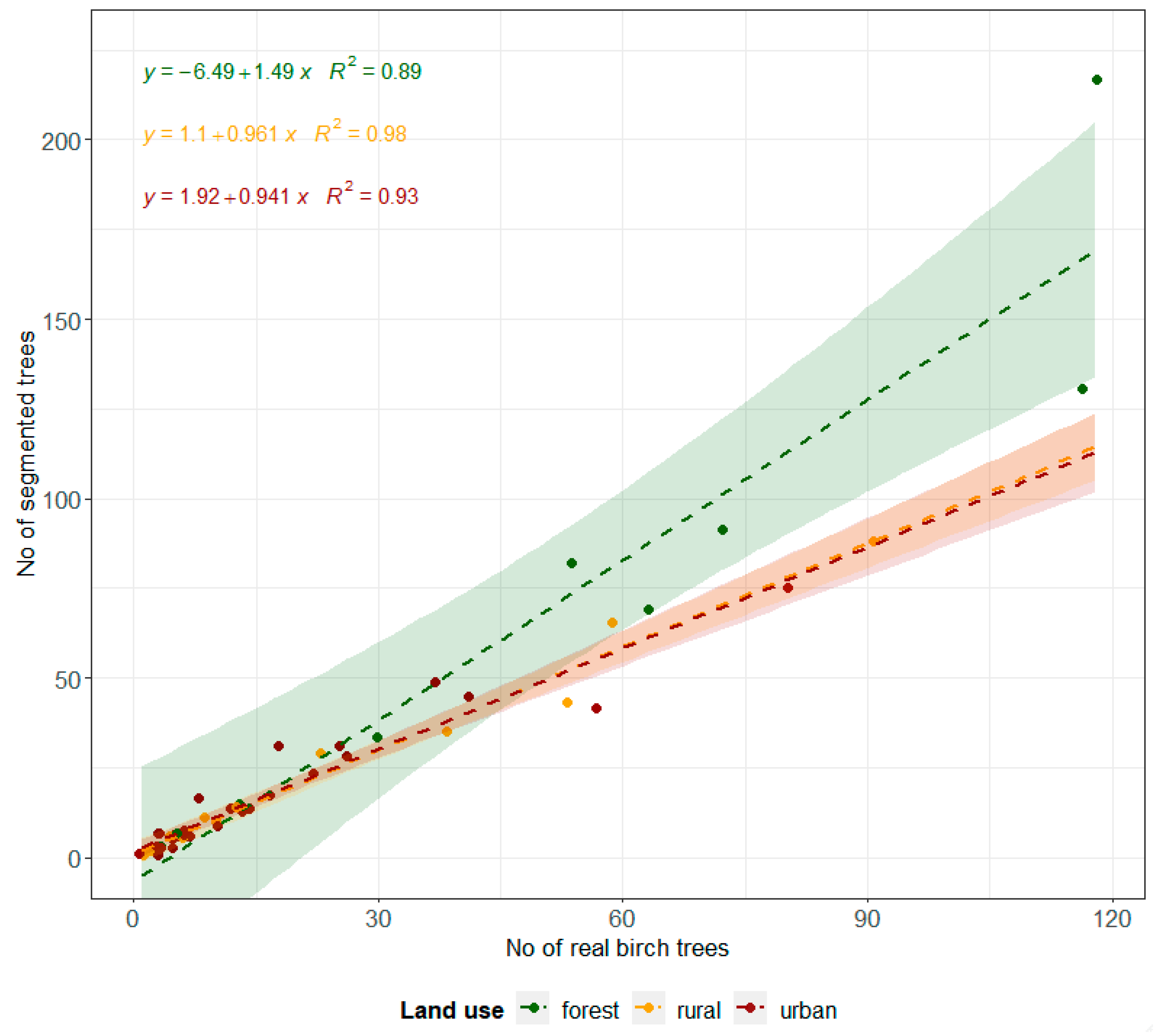
3.2. Birch Inventory

In total, based on LiDAR data, we delineated 18,740 birch trees that grew in 1693 groups within a 2-km radius from the pollen trap (Figure 1). The average birch tree density was 14.9 birch trees per 10,000 m2 in the study area. This value was very similar in urban and rural areas (11.2 and 11.3, respectively) but was markedly higher in forest areas (35.5). The highest tree density per 10,000 m2 was recorded in the SE sector from 1500 to 2000 m and from 500 to 1000 m from the pollen trap (65.8 and 25.8, respectively). There were also sectors with almost no birch trees, such as from 1500 to 2000 m to the N and from 500 to 1000 m to the NW (0.7 and 1.3, respectively) (Figure 4A). Trees were tallest in the NE and E sectors adjacent to the pollen trap and in the SE sector (distances of 500–1000 m and 1500–2000 m) and S sector (distances of 1500–2500 m) (Figure 4B).
We validated the individual crown delineation by comparing the number of delineated trees with the real number of trees in the field. In 48/100 plots, no birch trees were found. In the remaining 52 plots, at least one birch individual was noted, and a maximum of 118 trees were found in a plot. Generally, the observed and modelled number of birch trees agreed well with tree counts <30; however, for higher birch tree counts, these values were less similar. Nevertheless, the determination coefficient was high (r2 = 0.98 rural, r2 = 0.93 urban and r2 = 0.89 forest area), and the slope was close to 1 for rural and urban areas. However, the slope reached a = 1.49 in the forest area, meaning that the number of trees delineated based on LiDAR data was higher than the number of trees that actually grew in the field (Figure 5).

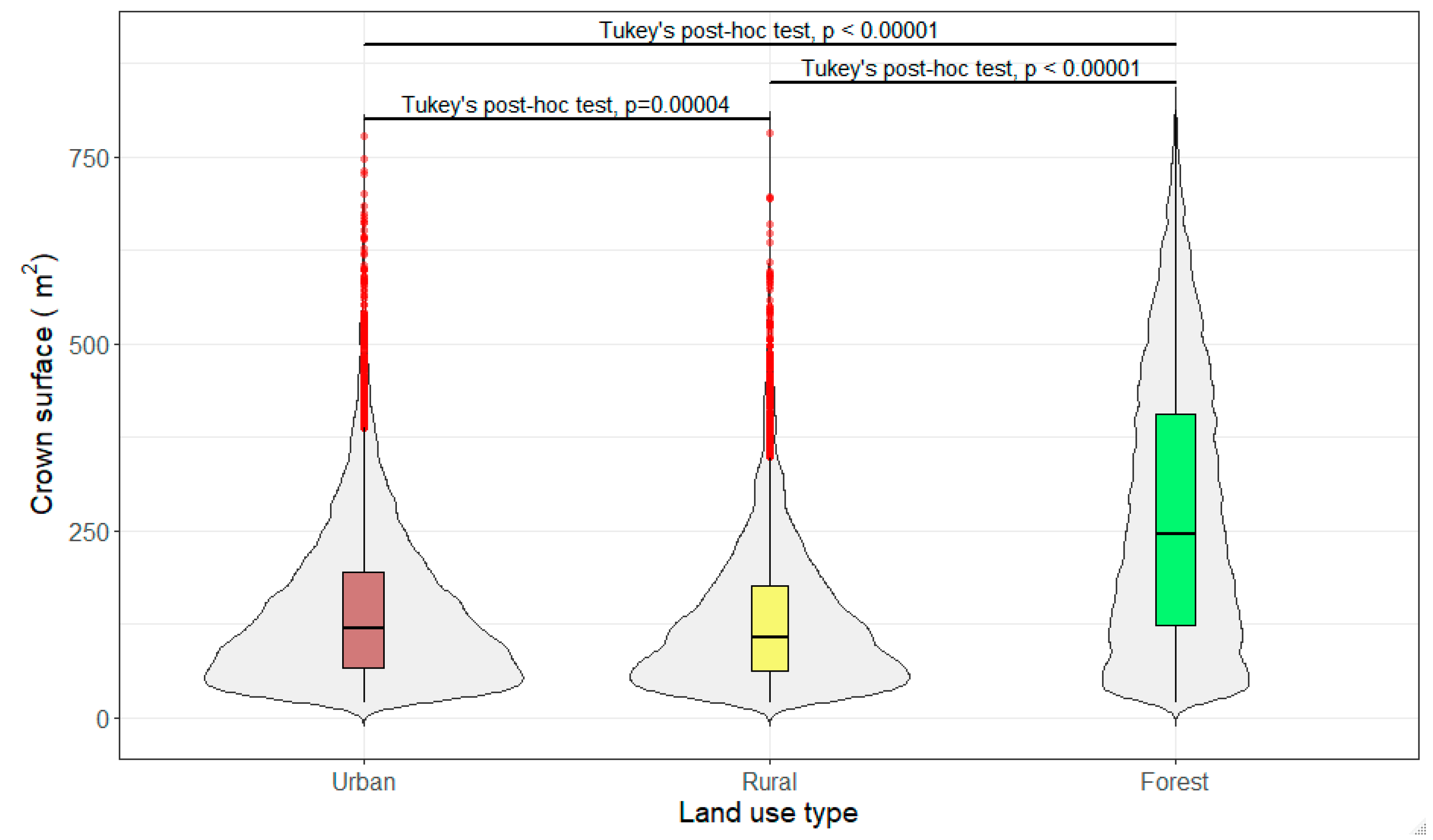
3.3. Crown Volume and Surface

The relationship between the birch crown volume and surface revealed similar patterns when compared among sectors or individuals (Table 1). Therefore, we focus on presenting the crown surface results in the text but present the results for the crown volumes in the figures and tables. The mean crown surface in forests (275.4 m2) was distinctly higher than that in urban and rural areas (146.0 and 133.9 m2, respectively) (F = 2158, p < 0.0001) (Figure 6). The largest mean birch crown surface values were noted in the SE and S sectors (251.6 and 217.9 m2, respectively), while the smallest crown surface values were noted in the NW and W sectors (114.8 and 125.4 m2, respectively). We also calculated the total birch crown surface per 100 m2 of ground surface in a sector as a function of the distance from the pollen trap; the SE sector from 1500 to 2000 m contained the largest birch crown surface (173.9 m2 per 100 m2 of ground surface). In almost all remaining sectors, the total birch crown surface was below 50 m2 per 100 m2 of ground surface (Figure 4C).

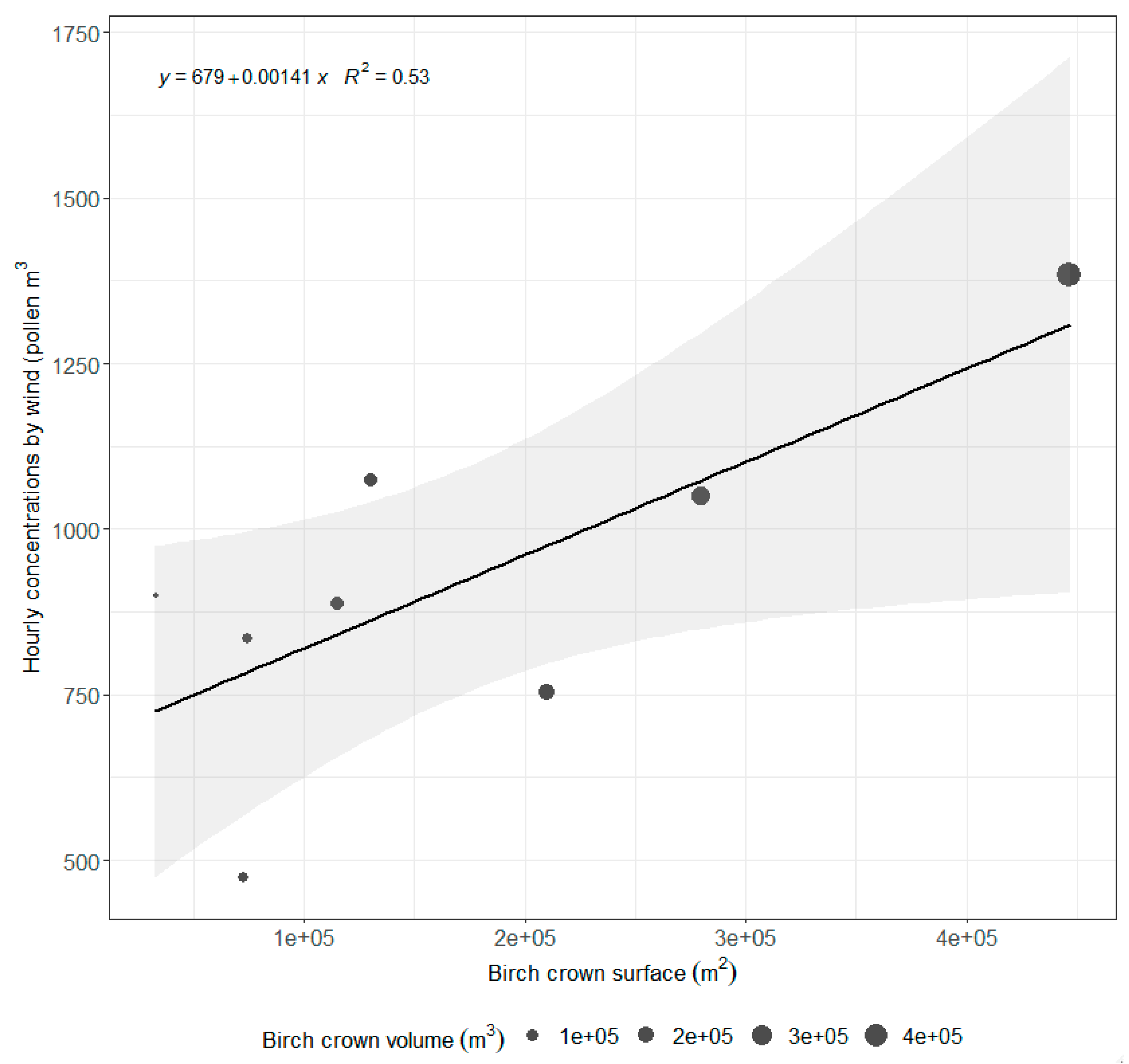
3.4. Relationship between Pollen Concentration and Birch Crown Parameters

The pollen concentrations attributed to the eight main wind directions were mostly positively correlated with the total crown surface and crown volume at different distances, but the relationships were not statistically significant (Table 2). The only statistically significant relationship was the correlation between the pollen concentration and the birch crown surface calculated for the area in the radius of 500–1500 m from the pollen trap (r = 0.728, p = 0.04) (Figure 7). Approximately the same values were obtained for the correlations between the pollen concentration and birch crown volume (Table 2).

4. Discussion

4.1. Impacts of Pollen Sources Vary in Space

In this study, we compared the pollen concentration based on the wind direction with the total birch crown surface and volume within a 2-km radius from the pollen trap. It was documented that the birch tree crown surface and volume in the 500–1500 m radius might impact the hourly pollen concentrations recorded during one pollen season. The settling velocity of birch pollen is low; thus, this pollen type can easily be transported long distances by wind [55,56]. For easily transported pollen types, it is believed that the source area that can influence the pollen concentration extends from 10 to 30–50 km from the receptor site [57,58]. Studies on Olea [59] and Quercus pollen [60] have shown that the highest correlation between the potential source area and pollen concentration occurs when considering the sources located 30–60 km (Olea sp.) or 10–20 km (Quercus sp.) away. The settling velocity, a parameter that describes the rate of sedimentation of the particles in the air, calculated by the method of Seinfield and Pandis [61], is 0.019 m s−1 for Olea pollen and 0.031 m s−1 for Quercus pollen [62]. The slower deposition of olive pollen results in a much larger area contributing to the pollen concentration at a receptor site for Olea sp. than for Quercus sp. Zhang et al. [62] also calculated the settling velocity for birch pollen, which was lower than that for Olea sp. (0.014 m s−1). Therefore, it is expected that the source area for birch pollen may extend beyond 60 km from the receptor site. In this study, we examined the area within a 2-km radius from the receptor site, which seems very small compared to the possible source area. However, Skjoth et al. [58] stressed that individual trees could cause high concentrations of airborne pollen in areas that were hundreds of metres from the source. This result was confirmed by the high amount of pollen deposited within 100 m from a tree relative to that deposited at greater distances [63]. Maya-Manzano et al. [26] assumed that the highest influence on olive, plane and cypress pollen concentrations in urban sites occurred within a distance of 500 m from the pollen monitoring site. In their study, it was revealed that the pollen concentration aggregated for all tree taxa excluding Quercus sp. was significantly related to the number of trees growing within a distance of 400–500 m from the monitoring site. In the present study, we also divided the study area into circles and annuli at different distances from the receptor site, at intervals of 500 m. Moreover, we included not only the number of trees as a measure of source size but also the total tree crown volume and surface in sectors located in the eight main directions. When using the tree crown surface, we obtained a higher Pearson correlation coefficient with pollen concentration (r = 0.728) than that reported in the study of Maya-Manzano et al. [26] (r = 0.466). It is possible that the latter correlation coefficient would be higher when considering a radius larger than 500 m from the pollen trap, as this coefficient increased with increasing distance [26]. The significant relationships between the pollen concentration and the pollen source area or surface/volume in a distance of 400 –500 m [26] or 500–1500 m (this study) from the pollen station showed that local near-sources over urban/semi-urban areas might considerably contribute to the pollen loads in cities, even for easily transported pollen such as that of Betula. However, it should be emphasized that these results are location specific. In other locations with different topography, land use, the spatial distribution of primary source plants, and the distance between the primary contributing pollen sources and receptor sites may be different. Nevertheless, allergy sufferers should be aware that allergenic trees growing within a 1500 m distance may be the primary cause of their allergy symptoms.

4.2. Birch Trees in Different Land-Use Types

Typically, pollen inventories are created based on the presence of birch trees within forests [11,14,22]. However, the potential influence of birch trees growing in urban areas on pollen count was previously mentioned by Corden et al. [64] and was confirmed by the analysis of Skjoth et al. [21]. In this study, we counted the number of birch trees growing in forests and in urban and rural areas. The individual tree delineation (ITD) in mixed forest areas showed high uncertainty because birch tree crowns sometimes overlapped with the crowns of other species (Figure 5). Nevertheless, based on LiDAR-derived ITD, the density of birch trees was at least three times higher in forests than in urban and rural areas. However, this result is a generalisation based only on the results from small, city outskirts area containing urban, rural and forest land-use types. This area may be treated as being representative of the outer zones of cities or suburbs. In such places, forests occupy a limited space and may not reflect the species composition of forests that are not adjacent to the city. Additionally, the density of birch may markedly vary not only between regions [65] but also between different urban areas, accounting for 3%–39% of all urban trees [24]. Nevertheless, we should be aware that substantial amounts of airborne birch pollen originate from trees growing outside of forests.
Considering a selection of large North American cities, ~20% of urban areas are covered by urban trees, and these areas may include urban parks, the regions along streets or residential areas [66]. The advantages of urban trees are indisputable: they reduce the urban heat island effect, reduce stormwater runoff and reduce flood effects; additionally, urban trees filter air pollution, limit the noise level and offer recreational sites for city inhabitants [67,68,69,70]. In Northern Europe, birch trees account for ~10% of trees inventoried within city streets and parks. Additionally, other allergenic species, such as Quercus, Fagus, Platanus, Salix, and Fraxinus, are commonly found in cities and constitute nearly 50% of the genera that are used for planting trees in cities [24]. Allergenic species are often planted in monospecific groups; these groups form large pollen emission sources and produce large amounts of pollen that cannot be removed from the city under specific meteorological conditions [71]. When planning urban green areas and selecting tree species, the needs of allergy sufferers are rarely considered [72,73]. Allergenic tree species are commonly planted in cities [74], and birch is a great example because of its ornamental functions and resistance to air pollution [75,76]. The results of the present study emphasise the importance of inventorying urban allergenic tree species; specifically, the pollen concentration was relatively high when we considered the winds blowing from Poznań city to the pollen trap in the city outskirts (Table 1).

4.3. Vertical Dimension of the Pollen Inventory—the Use of LiDAR Data

In this study, we inventoried (nearly) all birch trees growing within a distance of 2 km from a pollen trap in urban, rural and forested areas. Moreover, we calculated the external surfaces of their crowns. The age-related changes in the architecture of birch branches and the location of male catkins at terminal positions of a long shoot cause most of the male catkins to be within the external surface of the crown [77]. In this case, the external surface of a tree can act as a pollen emission surface. Therefore, we can assume that the external surface of a crown can be a proxy of pollen production of that tree. This assumption seems to be particularly important when the tree distribution is scattered. A scattered tree distribution causes the unconstrained development of branches, foliage and inflorescences and, therefore, results in a higher pollen production [78]. The birch trees growing at lower densities can increase the crown size up to two times compared to that of the trees growing in dense forests [79]. In our study, we generally calculated higher crown surfaces in forests than in rural and urban areas. This difference may result from the age (height) of the trees; for example, in our case, the forest trees were older than most of the trees growing in open areas (Figure 4B). Another explanation could be the management practices, as many of the urban trees are regularly trimmed, which reduces the crown size. However, it should be noted that trees with large crowns can also be found in open areas, but they are not as frequent as those found in forests. The large median tree crown surface of forest trees may not necessarily reflect high pollen production. As observed and simulated in Lintunen et al. [80], birch trees growing in forests under moderate competition reduce the number of branches in the lower parts of the crown, and many of these branches die. Moreover, the pollen emission is very limited from catkins developing under the canopy because of the reduced wind speed and high surface roughness [81]. Therefore, it seems that the lower parts of forest tree crowns should not be incorporated into a pollen inventory. Nevertheless, we suggest incorporating the third (vertical) dimension when creating pollen inventories; the tree crown surface should be used as an additional variable for estimating pollen emission and explaining local pollen concentration variability.

4.4. Limitations of the Study and Future Work

This study shows that it is possible to estimate the crown surface and volume as well as the number of trees from a large area using LiDAR data. It would be almost impossible to measure more than 18,000 trees in the field. However, we are aware that the method we proposed in this study requires optimisation. First, the birch crown surface should be reduced in birch trees growing in forests, and further work is required to determine which parts of a forest tree are important contributors of pollen. Second, we used only one individual crown delineation algorithm by Li et al. [49] with default parameters. The validation of this method in our case indicated that the results were similar to those obtained in the original study (r2 > 0.89). In open areas, the number of real and algorithmically delineated birch trees agreed well, while the number of trees was overestimated in dense forest stands (Figure 6). The adjustment of the method parameters will likely improve the quality of ITD. Moreover, there are also other methods for ITD, such as watershed ITD or the methods of Dalponte et al. [82] or Silva et al. [83]. However, the comparison of different ITD methods was beyond the scope of this study, but it is important for future work.
The assumption that crown surface is a predictor of pollen emission can also be biased by different numbers of catkins on trees of the same size. Ranta et al. [10] and Yasaka et al. [78] estimated that the number of catkins varies between years, which impacts the airborne pollen count. This variation implies that the crown surface may not be the only predictor of pollen emission, but it must be combined with other variables, such as phenological or meteorological data, that can explain the year-to-year variation in pollen count [84]. Recently, a terrestrial LiDAR system was also used to measure the pollen emissions from trees [85]. It is likely that it will be possible to estimate pollen emissions at their source by a combination of aerial and terrestrial LiDAR in the future.
Changes in temperature, precipitation or humidity during the study period could introduce another potential bias to the results because these variables affect the release and transport of pollen [86]. Days with low humidity and no precipitation favour the release of pollen from anthers, resulting in elevated pollen concentrations in the air [87]. Thus, due to the changing weather, the pollen emissions were not uniform during the study period. However, the use of a large data pool covering various meteorological conditions decreases the bias resulting from the uneven distribution of meteorological variables in the study period. In this study, we used 638 data points (hourly resolution of meteorological and pollen data) which is a high number, that covered different possible meteorological conditions in April. Therefore, we did not consider meteorological variables other than wind speed and direction to be necessary to assess the potential origin of pollen.
In the future, we plan to continue studies using LiDAR data for predicting pollen concentrations for birch and other tree species by creating a potentially complete inventory of urban allergenic trees. This research could be further used to quantify the impact of urban allergenic trees on pollen concentration and their contribution to the total pollen emission, which is an important component of pollen forecasting models.

5. Conclusions

This is the first study that quantifies the possible influence of LiDAR-derived crown surface and volume combined with wind direction on birch pollen concentrations at a suburban site. We documented a statistically significant relationship between the pollen concentration aggregated by wind direction and birch tree surface or volume within a distance of 500–1500 m from a pollen monitoring station. This result implies that a LiDAR-derived crown surface may be used as an additional variable for explaining pollen concentration variability. We also showed that birch trees were abundant not only in forests but also in urban and rural areas, with a density relationship of 3:1:1 for forest, urban and rural areas, respectively. The LiDAR-derived number of trees agreed well with the real number of trees, but the results were better at lower tree densities. We emphasise that urban and rural areas should be incorporated into pollen inventories, as they could substantially contribute to the total pollen emission. Moreover, we recommend adding the vertical dimension when creating pollen inventories, as this could improve the estimated pollen emissions. Further work is required to optimise the individual tree delineation algorithms for different land-use types and the tree-density-dependent fraction of crowns that may act as potential pollen emission surfaces.

Author Contributions

P.B. conceived and designed the study; P.B., Ł.G., K.D., K.S., M.D., B.D., D.P., A.N., M.N., A.S., Ł.K., M.M.N., B.J. were involved in data preparation, P.B., K.D., K.S., M.D. processed the data, K.S., M.D., B.D., D.P., A.N. were involved in field works, P.B. analysed the data, P.B., K.D., K.S., M.D. validated the results, P.B. prepared maps and figures; P.B. wrote the paper with the help of all co-authors.

Funding

This research received no external funding.

Acknowledgments

We would like to appreciate the work during the mapping of birch trees and the validation of the birch tree locations that was performed by Kamil Górny, Weronika Wasińska, Alicja Czerniak, Patryk Pawlak, Adam Berezowski and Angelika Pawlak.

Conflicts of Interest

The authors declare no conflict of interest.

References

  1. Beck, P.; Caudullo, G.; de Rigo, D.; Tinner, W. Betula pendula, Betula pubescens and other birches in Europe: Distribution, habitat, usage and threats. In European Atlas of Forest Tree Species; San-Miguel-Ayanz, J., de Rigo, D., Caudullo, G., Houston Durrant, T., Mauri, A., Eds.; Publication Office of the European Union: Luxembourg, 2016; p. e010226+. [Google Scholar]
  2. Atkinson, M.D. Betula Pendula Roth (B. Verrucosa Ehrh.) and B. Pubescens Ehrh. J. Ecol. 1992, 80, 837–870. [Google Scholar] [CrossRef]
  3. Burbach, G.J.; Heinzerling, L.M.; Edenharter, G.; Bachert, C.; Bindslev-Jensen, C.; Bonini, S. GA2LEN skin test study II: Clinical relevance of inhalant allergen sensitizations in Europe. Allergy 2009, 64, 1507–1515. [Google Scholar] [CrossRef] [PubMed]
  4. Warm, K.; Lindberg, A.; Lundbäck, B.; Rönmark, E. Increase in sensitization to common airborne allergens among adults—Two population-based studies 15 years apart. Allergy Asthma Clin. Immunol. 2013, 9, 20. [Google Scholar] [CrossRef] [PubMed] [Green Version]
  5. Rogers, C.A.; Wayne, P.M.; Macklin, E.A.; Muilenberg, M.L.; Wagner, C.J.; Epstein, P.R.; Bazzaz, F.A. Interaction of the Onset of Spring and Elevated Atmospheric CO2 On Ragweed (Ambrosia artemisiifolia L.) Pollen Production. Environ. Health Perspect. 2006, 114, 865–869. [Google Scholar] [CrossRef] [PubMed] [Green Version]
  6. Newnham, R.M.; Sparks, T.H.; Skjøth, C.A.; Head, K.; Adams-Groom, B.; Smith, M. Pollen season and climate: Is the timing of birch pollen release in the UK approaching its limit? Int. J. Biometeorol. 2013, 57, 391–400. [Google Scholar] [CrossRef]
  7. Pfaar, O.; Bastl, K.; Berger, U.; Buters, J.; Calderon, M.A.; Clot, B.; Darsow, U.; Demoly, P.; Durham, S.R.; Galan, C. Defining pollen exposure times for clinical trials of allergen immunotherapy for pollen-induced rhinoconjunctivitis—An EAACI Position Paper. Allergy 2017, 72, 713–722. [Google Scholar] [CrossRef]
  8. Sofiev, M.; Siljamo, P.; Ranta, H.; Rantio-Lehtimaki, A. Towards numerical forecasting of long-range air transport of birch pollen: Theoretical considerations and a feasibility study. Int. J. Biometeorol. 2006, 50, 392–402. [Google Scholar] [CrossRef]
  9. Bogawski, P.; Borycka, K.; Grewling, Ł.; Kasprzyk, I. Detecting distant sources of airborne pollen for Poland: Integrating back-trajectory and dispersion modelling with a satellite-based phenology. Sci. Total Environ. 2019, 689, 109–125. [Google Scholar] [CrossRef]
  10. Ranta, H.; Hokkanen, T.; Linkosalo, T.; Laukkanen, L.; Bondestam, K.; Oksanen, A. Male flowering of birch: Spatial synchronization, year-to-year variation and relation of catkins numbers and airborne pollen counts. For. Ecol. Manag. 2008, 255, 643–650. [Google Scholar] [CrossRef]
  11. Siljamo, P.; Sofiev, M.; Severova, E.; Ranta, H.; Kukkonen, J.; Polevova, S.; Kubin, E.; Minin, A. Sources, impact and exchange of early-spring birch pollen in the Moscow region and Finland. Aerobiologia 2008, 24, 211–230. [Google Scholar] [CrossRef]
  12. Skjøth, C.A.; Bilińska, D.; Werner, M.; Malkiewicz, M.; Adams-Groom, B.; Kryza, M.; Drzeniecka-Osiadacz, A. Footprint areas of pollen from alder (Alnus) and birch (Betula) in the UK (Worcester) and Poland (Wroclaw) during 2005–2014. Acta Agrobot. 2015, 68, 315–324. [Google Scholar] [CrossRef]
  13. Sofiev, M.; Vira, J.; Kouznetsov, R.; Prank, M.; Soares, J.; Genikhovich, E. Construction of the SILAM Eulerian atmospheric dispersion model based on the advection algorithm of Michael Galperin. Geosci. Model Dev. 2015, 8, 3497–3522. [Google Scholar] [CrossRef] [Green Version]
  14. Siljamo, P.; Sofiev, M.; Filatova, E.; Grewling, Ł.; Jäger, S.; Khoreva, E.; Linkosalo, T.; Ortega Jimenez, S.; Ranta, H.; Rantio-Lehtimäki, A.; et al. A numerical model of birch pollen emission and dispersion in the atmosphere. Model. Eval. Sensit. Anal. Int. J. Biometeorol. 2013, 57, 125–136. [Google Scholar] [CrossRef] [PubMed] [Green Version]
  15. Skjoth, C.A.; Šikoparija, B.; Jager, S. EAN-Network Chapter 2. Pollen Sources. In Allergenic Pollen: A Review of the Production, Release, Distribution and Health Impacts; Sofiev, M., Bergmann, K.C., Eds.; Springer Science+Business Media: Dordrecht, The Nederlands, 2013. [Google Scholar]
  16. Ritenberga, O.; Sofiev, M.; Kirillova, V.; Kalnina, L.; Genikhovich, E. Statistical modelling of non-stationary processes of atmospheric pollution from natural sources: Example of birch pollen. Agric. For. Meteorol. 2016, 226, 96–107. [Google Scholar] [CrossRef]
  17. De Rigo, D.; Caudullo, G.; Houston Durrant, T.; San-Miguel-Ayanz, J. The European Atlas of Forest Tree Species: Modelling, data and information on forest tree species. In European Atlas of Forest Tree Species; San-Miguel-Ayanz, J., de Rigo, D., Caudullo, G., Houston Durrant, T., Mauri, A., Eds.; Publication Office of the European Union: Luxembourg, 2016; p. e01aa69+. [Google Scholar]
  18. McInnes, R.N.; Hemming, D.; Burgess, P.; Lyndsay, D.; Osborne, N.J.; Skjøth, C.A.; Thomas, S.; Vardoulakis, S. Mapping allergenic pollen vegetation in UK to study environmental exposure and human health. Sci. Total Environ. 2017, 599, 483–499. [Google Scholar] [CrossRef] [PubMed] [Green Version]
  19. Skjøth, C.S.; Sun, Y.; Karrer, G.; Sikoparija, B.; Smith, M.; Schaffner, U.; Müller-Schärer, H. Predicting abundances of invasive ragweed across Europe using a “top-down” approach. Sci. Total Environ. 2019, 686, 212–222. [Google Scholar] [CrossRef] [Green Version]
  20. Jackowiak, B. Atlas of Distribution of Vascular Plants in Poznań; No. 2; The Department of Plant Taxonomy of the Adam Mickiewicz University: Poznań, Poland, 1993; p. 409. [Google Scholar]
  21. Skjøth, C.A.; Sommer, J.; Brandt, J.; Hvidberg, M.; Geels, C.; Hansen, K.M.; Hertel, O.; Frohn, L.M.; Christensen, J.H. CopenhagenA significant source to birch (Betula) pollen? Int. J. Biometeorol. 2008, 52, 453–462. [Google Scholar] [CrossRef]
  22. Skjøth, C.A.; Geels, C.; Hvidberg, M.; Hertel, O.; Brandt, J.; Frohn, L.M.; Hansen, K.M.; Hedegaard, G.B.; Christensen, J.; Moseholm, L. An inventory of tree species in EuropeAn essential data input for air pollution modelling. Ecol. Model. 2008, 217, 292–304. [Google Scholar] [CrossRef]
  23. Skjøth, C.A.; Ørby, P.V.; Becker, T.; Geels, C.; Schlunssen, V. Identifying urban sources as cause of elevated grass pollen concentrations using GIS and remote sensing. Biogeosciences 2013, 10, 541–554. [Google Scholar] [CrossRef] [Green Version]
  24. Sjöman, H.; Östberg, J.; Bühler, O. Diversity and distribution of the urban tree population in ten major Nordic cities. Urban For. Urban Green. 2012, 11, 31–39. [Google Scholar]
  25. Pecero-Casimiro, R.; Fernández-Rodríguez, S.; Tormo-Molina, R.; Monroy-Colín, A.; Silva-Palacios, I.; Cortés-Pérez, J.P.; Gonzalo-Garijo, A.; Maya-Manzano, J.-M. Urban aerobiological risk mapping of ornamental trees using a new index based on LiDAR and Kriging: A case study of plane trees. Sci. Total Environ. 2019, 693, 133576. [Google Scholar] [CrossRef] [PubMed]
  26. Maya-Manzano, J.M.; Tormo-Molina, R.; Rodríguez, S.F.; Palacios, I.S.; Garijo, Á.G. Distribution of ornamental urban trees and their influence on airborne pollen in the SW of Iberian Peninsula. Landsc. Urban Plan. 2017, 157, 434–446. [Google Scholar] [CrossRef]
  27. Matthias, I.; Nielsen, A.B.; Giesecke, T. Evaluating the effect of flowering age and forest structure on pollen productivity estimates. Veget. Hist. Archaeobot. 2012, 21, 471–484. [Google Scholar] [CrossRef] [Green Version]
  28. Longman, K.A.; Wareing, P.F. Early Induction of Flowering in Birch Seedlings. Nature 1959, 184, 203. [Google Scholar] [CrossRef]
  29. Carson, W.W.; Andersen, H.-E.; Reutebuch, S.E.; McGaughey, R.J. Lidar Applications In ForestryAn Overview 7-2038. In Proceedings of the ASPRS Annual Conference Proceedings, Denver, CO, USA, 23–28 May 2004. [Google Scholar]
  30. Vauhkonen, J.; Maltamo, M.; McRoberts, R.E.; Næsset, E. Chapter 1: Introduction to Forestry Applications of Airborne Laser Scanning. In Concepts and Case Studies, Managing Forest Ecosystems; Maltamo, M., Næsset, E., Vauhkonen, J., Eds.; Springer Science+Business Media: Dordrecht, The Nederlands, 2014; Volume 27. [Google Scholar]
  31. MacFaden, S.W.; O’Neil-Dunne, J.P.M.; Royar, A.R.; Lu, J.W.T.; Rundle, A.G. High-resolution tree canopy mapping for New York City using LIDAR and object-based image analysis. J. Appl. Remote Sens. 2012, 6, 063567. [Google Scholar] [CrossRef]
  32. Vaughn, N.R.; Moskal, M.; Turnblom, E.C. Tree Species Detection Accuracies Using Discrete Point Lidar and Airborne Waveform Lidar. Remote Sens. 2012, 4, 377–403. [Google Scholar] [CrossRef] [Green Version]
  33. Donager, J.J.; Sankey, T.T.; Sankey, J.B.; Sanchez Meador, A.J.; Springer, A.E.; Bailey, J.D. Examining Forest Structure With Terrestrial Lidar: Suggestions and Novel Techniques Based on Comparisons Between Scanners and Forest Treatments. Earth Space Sci. 2018, 5, 753–776. [Google Scholar] [CrossRef] [Green Version]
  34. Shang, X.; Chazette, P. Interest of a full-waveform flown UV lidar to derive forest vertical structures and aboveground carbon. Forests 2014, 5, 1454–1480. [Google Scholar] [CrossRef] [Green Version]
  35. Hancock, S.; Armston, J.; Hofton, M.; Sun, X.; Tang, H.; Duncanson, L.I.; Kellner, J.R.; Dubayah, R. The GEDI Simulator: A Large-Footprint Waveform Lidar Simulator for Calibration and Validation of Spaceborne Missions. Earth Space Sci. 2019, 6, 294–310. [Google Scholar] [CrossRef]
  36. Roncat, A.; Morsdorf, F.; Briese, C.; Wagner, W.; Pfeifer, N. Chapter 2. Laser Pulse Interaction with Forest Canopy: Geometric and Radiometric Issues. In Forestry Applications of Airborne Laser Scanning; Maltamo, M., Næsset, E., Vauhkonen, J., Eds.; Concepts and Case Studies, Managing Forest Ecosystems; Springer Science+Business Media: Dordrecht, The Nederlands, 2014. [Google Scholar]
  37. Kottek, M.; Grieser, J.; Beck, C.; Rudolf, B.; Rubel, F. World Map of the Köppen-Geiger climate classification updated. Meteorol. Z. 2006, 15, 259–263. [Google Scholar] [CrossRef]
  38. Woś, A. Klimat Polski w drugiej połowie XX wieku; Wyd. Naukowe UAM: Poznań, Poland, 2010. [Google Scholar]
  39. Kolendowicz, L.; Czernecki, B.; Półrolniczak, M.; Taszarek, M.; Tomczyk, A.M.; Szyga-Pluga, K. Homogenization of air temperature and its long-term trends in Poznań (Poland) for the period 1848–2016. Theor. Appl. Climatol. 2019, 136, 1357–1370. [Google Scholar] [CrossRef] [Green Version]
  40. Hirst, J.M. An automatic volumetric spore trap. Ann. Appl. Biol. 1952, 39, 257–265. [Google Scholar] [CrossRef]
  41. Galán, C.; Smith, M.; Thibaudon, M.; Frenguelli, G.; Oteros, J.; Gehrig, R.; Berger, U.; Clot, B.; Brandao, R.; EAS QC Working Group. Pollen monitoring: Minimum requirements and reproducibility of analysis. Aerobiologia 2014, 30, 385–395. [Google Scholar]
  42. Uria-Tellaetxe, I.; Carslaw, D.C. Conditional bivariate probability function for source identification. Environ. Model. Softw. 2014, 59, 1–9. [Google Scholar] [CrossRef] [Green Version]
  43. Carslaw, D.C.; Beevers, S.D. Characterising and understanding emission sources using bivariate polar plots and k-means clustering. Environ. Model. Softw. 2013, 40, 325–329. [Google Scholar] [CrossRef]
  44. Carslaw, D.C.; Ropkins, K. OpenairAn R package for air quality data analysis. Environ. Model. Softw. 2012, 27, 52–61. [Google Scholar] [CrossRef]
  45. Google. Explore Street View. 2018. Available online: https://www.google.com/maps/streetview/explore/ (accessed on 15 February 2019).
  46. European Environment Agency (EEA); European Union. Copernicus Land Monitoring Service CORINE Land Cover. 2012,dataset. Available online: www.eea.europa.eu/data-and-maps/data/copernicus-land-monitoring-service-corine (accessed on 18 May 2019).
  47. Wężyk, P. (Ed.) Podręcznik dla uczestników szkoleń z wykorzystania produktów LiDAR; Główny Urząd Geodezji i Kartografii: Warszawa, Poland, 2015. (In Polish) [Google Scholar]
  48. Roussel, J.-R.; Auty, D. lidR: Airborne LiDAR Data Manipulation and Visualization for Forestry Applications. R Package Version 2.0.3; Repository: CRAN. 2019. Available online: https://cran.r-project.org/web/packages/lidR/index.html (accessed on 11 November 2019).
  49. Li, W.; Guo, Q.; Jakubowski, M.K.; Kelly, M. A new method for segmenting individual trees from the lidar point cloud. Photogramm. Eng. Remote Sens. 2012, 78, 75–84. [Google Scholar] [CrossRef] [Green Version]
  50. Barber, C.B.; Dobkin, D.P.; Huhdanpaa, H.T. The Quickhull algorithm for convex hulls. ACM Trans. Math. Softw. 1996, 22, 469–483. [Google Scholar] [CrossRef] [Green Version]
  51. R Core Team. A Language and Environment for Statistical Computing; R Foundation for Statistical Computing: Vienna, Austria, 2018; Available online: https://www.R-project.org/ (accessed on 30 July 2018).
  52. Silva, C.A.; Crookston, N.L.; Hudak, A.T.; Vierling, L.A.; Klauberg, C.; Cardil, A. rLiDAR: LiDAR Data Processing and Visualization. R Package Version 0.1.1; Repository: CRAN. 2017. Available online: https://cran.r-project.org/web/packages/rLiDAR/index.html (accessed on 11 November 2019).
  53. Habel, K.; Grasman, R.; Gramacy, R.B.; Stahel, A.; Sterratt, D.C. Geometry: Mesh Generation and Surface Tesselation. R Package Version 0.3-6; Repository: CRAN. 2015. Available online: https://cran.r-project.org/web/packages/geometry/index.html (accessed on 11 November 2019).
  54. Elzinga, C.L.; Salzer, D.W.; Willoughby, J.W. Measuring & monitoring plant populations; U.S. Bureau of Land Management; Papers 17; University of Nebraska Lincoln: Lincoln, NE, USA, 1998. [Google Scholar]
  55. Jackson, S.T.; Lyford, M. Pollen Dispersal Models in Quaternary Plant Ecology: Assumptions, Parameters, and Prescriptions. Bot. Rev. 1999, 65, 39–75. [Google Scholar] [CrossRef]
  56. Skjøth, C.A.; Sommer, J.; Stach, A.; Smith, M.; Brandt, J. The long range transport of birch (Betula) pollen from Poland and Germany causes significant pre-season concentrations in Denmark. Clin. Exp. Allergy 2007, 37, 1204–1212. [Google Scholar] [CrossRef] [Green Version]
  57. Maya-Manzano, J.M.; Sadyś, M.; Tormo-Molina, R.; Fernández-Rodríguez, S.; Oteros, J.; Silva-Palacios, I.; Gonzalo-Garijo, A. Relationships between airborne pollen grains, wind direction and land cover using GIS and circular statistics. Sci. Total Environ. 2017, 584, 603–613. [Google Scholar] [CrossRef] [PubMed]
  58. Skjøth, C.A.; Baker, P.; Sadyś, M.; Adams-Groom, B. Pollen from alder (Alnus sp.), birch (Betula sp.) and oak (Quercus sp.) in the UK originate from small woodlands. Urban Clim. 2015, 14, 414–428. [Google Scholar]
  59. Oteros, J.; García-Mozo, H.; Alcázar, P.; Belmonte, J.; Bermejo, D.; Boi, M.; Cariñanos, P.; de la Guardia, C.D.; Fernández-González, D.; González-Minero, F.; et al. A new method for determining the sources of airborne particles. J. Environ. Manag. 2015, 155, 212–218. [Google Scholar] [CrossRef] [PubMed]
  60. Oteros, J.; Valencia, R.M.; del Río, S.; Vega, A.M.; García-Mozoc, H.; Galánc, C.; Gutiérrez, P.; Mandrioli, P.; Fernández-González, D. Concentric Ring Method for generating pollen maps. Quercus as case study. Sci. Total Environ. 2017, 576, 637–645. [Google Scholar] [CrossRef] [PubMed]
  61. Seinfeld, J.; Pandis, S. Atmospheric Chemistry and Physics; Wiley: New York, NY, USA, 1998. [Google Scholar]
  62. Zhang, R.; Duhl, T.; Salam, M.T.; House, J.M.; Flagan, R.C.; Avol, E.L.; Gilliland, F.D.; Guenther, A.; Chung, S.H.; Lamb, B.K.; et al. Development of a regional-scale pollen emission and transport modeling framework for investigating the impact of climate change on allergic airway disease. Biogeosciences 2014, 11, 1461–1478. [Google Scholar] [CrossRef] [Green Version]
  63. Adams-Groom, B.; Skjøth, C.; Baker, M.; Welch, T.E. Modelled and Observed Surface Soil Pollen Deposition Distance Curves for Isolated Trees of Carpinus Betulus, Cedrus Atlantica, Juglans nigra and Platanus Acerifolia. Aerobiologia 2017, 33, 407–416. [Google Scholar] [CrossRef]
  64. Corden, J.; Millington, W.; Bailey, J.; Brookes, M.; Caulton, E.; Emberlin, J.; Mullins, J.; Simpson, C.; Wood, A. UK regional variations in Betula pollen (1993–1997). Aerobiologia 2000, 16, 227–232. [Google Scholar] [CrossRef]
  65. Zajączkowski, S.; Talarczyk, A.; Myszkowski, M.; Kucab, M. Wyniki aktualizacji stanu powierzchni leśnej i zasobów drzewnych w Lasach Państwowych na dzień 1 stycznia 2018 r; Oficyna wydawnicza Forest: Sękocin Stary, Poland, 2019. [Google Scholar]
  66. Nowak, D.J.; Hoehn, R.E.; Crane, D.E.; Stevens, J.C.; Walton, J.T. Northern Resource Bulletin NRS-8. In Assessing Urban Forest Effects and Values: San Francisco’s Urban Forest; USDA Forest Service: Newtown Square, PA, USA, 2007; p. 24. [Google Scholar]
  67. Tyrväinen, L.; Mäkinen, L.; Schipperijn, J. Tools for mapping social values for urban woodlands and of other green spaces. Landsc. Urban. Plan. 2007, 79, 5–19. [Google Scholar] [CrossRef]
  68. Selmi, W.; Weber, C.; Rivière, E.; Blond, N.; Mehdi, L.; Nowak, D. Air pollution removal by trees in public green spaces in Strasbourg City, France. Urban For. Urban Green. 2016, 17, 192–201. [Google Scholar] [CrossRef] [Green Version]
  69. Ow, L.F.; Ghosh, S. Urban cities and road traffic noise: Reduction through vegetation. Appl. Acoust. 2017, 120, 15–20. [Google Scholar] [CrossRef]
  70. Elmqvist, T.; Setälä, H.; Handel, S.N.; van der Ploeg, S.; Aronson, J.; Blignaut, J.N.; Gómez-Baggethun, E.; Nowak, D.J.; Kronenberg, J.; de Groot, R. Benefits of restoring ecosystem services in urban areas. Curr. Opin. Environ. Sustain. 2015, 14, 101–108. [Google Scholar]
  71. Carinanos, P.; Casares-Porcel, M. Urban green zones and related pollen allergy: A review. Some guidelines for designing spaces with low allergy impact. Landsc. Urban Plan. 2011, 101, 205–214. [Google Scholar] [CrossRef]
  72. Pauleit, S.; Duhme, F. Assessing the environmental performance of land cover types for urban planning. Landsc. Urban. Plan. 2000, 52, 1–20. [Google Scholar] [CrossRef]
  73. Sæbø, A.; Benedikz, T.; Randrup, T.B. Selection of trees for urban forestry in the Nordic countries. Urban. For. Urban. Green. 2003, 2, 101–114. [Google Scholar] [CrossRef] [Green Version]
  74. Jochner-Oette, S.; Stitz, T.; Jetschni, J.; Cariñanos, P. The Influence of Individual-Specific Plant Parameters and Species Composition on the Allergenic Potential of Urban Green Spaces. Forests 2018, 9, 284. [Google Scholar] [CrossRef] [Green Version]
  75. Kozlov, M.V.; Zvereva, E.L. Reproduction of mountain birch along a strong pollution gradient near Monchegorsk: Northwestern Russia. Environ. Pollut. 2004, 132, 443–451. [Google Scholar] [CrossRef] [PubMed]
  76. Eränen, J.K. Local adaptation of mountain birch to heavy metals in subarctic industrial barrens. For. Snow Landsc. Res. 2006, 80, 161–167. [Google Scholar]
  77. Kostina, M.V.; Barabanshikova, N.S.; Bityugova, G.V.; Yasinskaya, O.I.; Dubach, A.M. Structural Modifications of Birch (Betula pendula Roth.) Crown in Relation to Environmental Conditions. Contemp. Probl. Ecol. 2015, 8, 584–597. [Google Scholar] [CrossRef]
  78. Yasaka, M.; Kobayashi, S.; Takeuchi, S.; Tokuda, S.; Takiya, M.; Ohno, Y. Prediction of birch airborne pollen counts by examining male catkin numbers in Hokkaido, northern Japan. Aerobiologia 2009, 25, 111–117. [Google Scholar] [CrossRef]
  79. Ilomäki, S.; Nikinmaa, E.; Mäkelä, A. Crown rise due to competition drives biomass allocation in silver birch. Can. J. For. Res. 2003, 33, 2395–2404. [Google Scholar] [CrossRef]
  80. Lintunen, A.; Sievänen, R.; Kaitaniemi, P.; Perttunen, J. Models of 3D crown structure for Scots pine (Pinus sylvestris) and silver birch (Betula pendula) grown in mixed forest. Can. J. Res. 2011, 41, 1779–1794. [Google Scholar] [CrossRef]
  81. Michel, D. Observations and Modelling of Birch Pollen Emission and Dispersion from an Isolated Source. Ph.D. Thesis, University of Basel, Basel, Switzerland, 2014. [Google Scholar]
  82. Dalponte, M.; Coomes, D.A. Tree-centric mapping of forest carbon density from airborne laser scanning and hyperspectral data. Methods Ecol. Evol. 2016, 7, 1236–1245. [Google Scholar] [CrossRef] [PubMed] [Green Version]
  83. Silva, C.A.; Hudak, A.T.; Vierling, L.A.; Loudermilk, E.L.; O’Brien, J.J.; Hiers, J.K.; Khosravipour, A. Imputation of Individual Longleaf Pine (Pinus palustris Mill.) Tree Attributes from Field and LiDAR Data. Can. J. Remote Sens. 2016, 42, 554–573. [Google Scholar]
  84. Bogawski, P.; Grewling, Ł.; Jackowiak, B. Predicting the onset of Betula pendula flowering in Poznań (Poland) using remote sensing thermal data. Sci. Total Environ. 2019, 658, 1485–1499. [Google Scholar] [CrossRef] [PubMed]
  85. Bohlmann, S.; Shang, X.; Giannakaki, E.; Filioglou, M.; Saarto, A.; Romakkaniem, S.; Komppula, M. Detection and characterization of birch pollen in the atmosphere using multi-wavelength Raman lidar in Finland. Atmos. Chem. Phys. Discuss. 2019. [Google Scholar] [CrossRef] [Green Version]
  86. Robichaud, A.; Comtois, P. Statistical modeling, forecasting and time series analysis of birch phenology in Montreal, Canada. Aerobiologia 2017, 33, 529–554. [Google Scholar] [CrossRef]
  87. Grewling, L.; Jackowiak, B.; Nowak, M.; Uruska, A.; Smith, M. Variations and trends of birch pollen seasons during 15 years (1996–2010) in relation to weather conditions in Poznań (western Poland). Grana 2012, 51, 280–292. [Google Scholar] [CrossRef] [Green Version]
Figure 1. Study area.
Forests 10 01154 g001
Figure 2. Examples of birch tree stands in an open habitat (A) and in a forest (B) in the study area. The normalised point cloud is plotted as small colour points. The 3D shapes reflect individual segmented birch trees. Images on the right were acquired using Google Earth software.
Forests 10 01154 g002
Figure 3. Hourly birch pollen concentration in the outskirts of Poznań city in 2012 according to the wind direction and speed (A) and significant structures within the data considering different numbers of clusters determined on the basis of partitioning around medoids (B).
Forests 10 01154 g003
Figure 4. LiDAR derived mean values of crown parameters attributed to different sectors around the pollen monitoring site: A—birch tree density, B—birch tree height, C—birch tree crown surface and D—birch tree crown volume.
Forests 10 01154 g004
Figure 5. Validation of the tree segmentation based on counting trees in Google Earth and in the field for 52 randomly selected plots (100 plots were drawn, but 48 showed no birch trees). The confidence interval was at the 0.95 level.
Forests 10 01154 g005
Figure 6. Differences in crown surface between birch trees growing within different land-use types (Analysis of Variance (ANOVA), F = 1524, p < 0.0001). N = 18,740 segmented trees (6805 urban, 5202 agricultural area, 6733 forests).
Forests 10 01154 g006
Figure 7. Statistically significant relationship (p = 0.0406) between the hourly birch pollen concentration summed by the influx direction and the total birch crown surface within 500 to 1500 m from the pollen sampler.
Forests 10 01154 g007
Table 1. Descriptive statistics of birch tree crown volume and surface by sectors and the pollen concentration recorded by wind direction.
Descriptive StatisticWind Directions/Sectors
ENNENWSSESWW
Crown volume [m3]sum416,903.6253,275.2233,730.9148,841.3419,030.21,922,507168,407.4225,820.8
mean158.4161.1157.598.2243.6292.2136.3112.9
standard deviation194.0182.2191.6109.7282.4311.8149.6129.3
skewness2.62.22.32.91.91.52.02.3
min0.83.92.73.83.01.63.71.7
1st quartile33.537.933.526.541.958.531.427.7
median89.199.085.864.4131.8168.380.963.7
3rd quartile205.2215.4198.7131.4346.8433.0187.3150.4
max1561.81384.51267.51067.71645.11644.11038.2984.6
Crown surface [m2]sum419,437.7257,290.4236,891.4174,051.4374,786.61,655,425176,389.0250,973.5
mean159.4163.7159.6114.8217.9251.6142.7125.4
standard deviation122.4114.8124.277.4161.8176.297.589.7
skewness1.51.31.41.61.00.71.21.4
min20.020.820.120.120.120.020.120.2
1st quartile68.375.168.056.685.5104.966.858.7
median124.6134.8122.199.2172.9205.1118.9100.7
3rd quartile211.2219.2207.4151.9315.2375.9199.5166.1
max777.4695.2675.2588.2801.8812.7605.6565.0
Pollen [count per hour]total integrated hourly pollen count68,253.438,37221,125.869,143.888,372.2171,624.659,550.8112,964.2
no of hours with wind from the sector6551457710012471105
mean pollen count per hour1050.1752.4469.5898.0883.71384.1838.71075.8
Mean crown volume/pollen ratio6.634.672.989.143.634.746.159.53
Mean crown surface/pollen ratio6.594.602.947.824.065.505.888.58
Mean crown volume/surface ratio0.990.980.990.861.121.160.960.90
Table 2. Correlation coefficients between pollen concentrations in 2012 aggregated by wind direction and the LiDAR-derived crown volume and crown surface values for the corresponding wind direction and at different distances from the pollen sampler.
Distance to Pollen Sampler [m]Crown Surface in Sectors [m2]Crown Volume in Sectors [m3]
Correlation Coefficientp-ValueCorrelation Coefficientp-Value
From 0 to 500*cor = −0.3990.3268cor = −0.3830.3487
From 0 to 1000cor = 0.5920.1224cor = 0.5820.1302
From 500 to 1000cor = 0.7010.0526**rho = 0.5240.1966
From 0 to 1500cor = 0.6740.0668cor = 0.6700.0689
From 500 to 1500cor = 0.7280.0406cor = 0.7290.0399
From 1000 to 1500cor = 0.6830.0617cor = 0.6960.0554
From 0 to 2000rho = 0.4760.2431rho = 0.2860.5008
From 500 to 2000rho = 0.5950.1323rho = 0.4290.2992
From 1000 to 2000rho = 0.5710.1511rho = 0.4760.2431
From 1500 to 2000rho = 0.2860.5008rho = 0.2860.5008
*cor—Pearson correlation coefficient; **rho—Spearman correlation coefficient calculated when dataset did not follow a normal distribution (Shapiro-Wilk test, α = 0.05).

