Article

Nondestructive Estimation of the Above-Ground Biomass of Multiple Tree Species in Boreal Forests of China Using Terrestrial Laser Scanning

1
Precision Forestry Key Laboratory of Beijing, Beijing Forestry University, Beijing 100083, China
2
Mapping and 3S Technology Center, Beijing Forestry University, Beijing 100083, China
3
School of Nature Conservation, Beijing Forestry University, Beijing 100083, China
*
Author to whom correspondence should be addressed.
Forests 2019, 10(11), 936; https://doi.org/10.3390/f10110936
Submission received: 15 September 2019 / Revised: 9 October 2019 / Accepted: 19 October 2019 / Published: 23 October 2019

Abstract

:
Above-ground biomass (AGB) plays a pivotal role in assessing a forest’s resource dynamics, ecological value, carbon storage, and climate change effects. The traditional methods of AGB measurement are destructive, time consuming and laborious, and an efficient, relatively accurate and non-destructive AGB measurement method will provide an effective supplement for biomass calculation. Based on the real biophysical and morphological structures of trees, this paper adopted a non-destructive method based on terrestrial laser scanning (TLS) point cloud data to estimate the AGBs of multiple common tree species in boreal forests of China, and the effects of differences in bark roughness and trunk curvature on the estimation of the diameter at breast height (DBH) from TLS data were quantitatively analyzed. We optimized the quantitative structure model (QSM) algorithm based on 100 trees of multiple tree species, and then used it to estimate the volume of trees directly from the tree model reconstructed from point cloud data, and to calculate the AGBs of trees by using specific basic wood density values. Our results showed that the total DBH and tree height from the TLS data showed a good consistency with the measured data, since the bias, root mean square error (RMSE) and determination coefficient (R2) of the total DBH were −0.8 cm, 1.2 cm and 0.97, respectively. At the same time, the bias, RMSE and determination coefficient of the tree height were −0.4 m, 1.3 m and 0.90, respectively. The differences of bark roughness and trunk curvature had a small effect on DBH estimation from point cloud data. The AGB estimates from the TLS data showed strong agreement with the reference values, with the RMSE, coefficient of variation of root mean square error (CV(RMSE)), and concordance correlation coefficient (CCC) values of 17.4 kg, 13.6% and 0.97, respectively, indicating that this non-destructive method can accurately estimate tree AGBs and effectively calibrate new allometric biomass models. We believe that the results of this study will benefit forest managers in formulating management measures and accurately calculating the economic and ecological benefits of forests, and should promote the use of non-destructive methods to measure AGB of trees in China.

1. Introduction

Forest biomass is an important indicator of forest productivity, carbon storage and forest carbon sequestration capacity, and it has been widely investigated by the scientific community [1,2,3]. As a developing country, China has taken measures to increase forest biomass and carbon storage by limiting deforestation and afforestation, and positively supports and implements the mechanism of Reducing emissions from deforestation and forest degradation in developing countries (REDD+). Accurate assessment of forest biomass plays a pivotal role in afforestation management planning, forest resource monitoring, the assessment of the ecological value of forests, climate change impacts and policy formulation for forest harvesting, conservation and management [4,5]. The assessment of forest biomass includes the estimation of both above-ground biomass (AGB) and underground biomass. However, the underground biomass is not only difficult to quantify, but it is relatively small to the AGB [6]. Therefore, the estimation of AGB has always been the main focus in biomass research. AGB calculations rely on tree structure parameters, such as diameter at breast height (DBH), tree height, crown radius, etc., form which the AGB can be calculated using allometric biomass models, which can be very effective when applied to tree species and productivity ranges with reliable calibration data. Conventional methods for AGB measurement, which involve cutting down trees and then drying them for weighing, are destructive, time-consuming, expensive and laborious, and are consequently rarely adopted [7,8]. Moreover, the conventional methods can be used only for a small area, as their accuracy could be compromised when used to estimate the AGB of a forest spanning over a larger region [2,8,9,10,11].
The use of advanced technologies in forestry, especially remote sensing technology, provides an alternative tool to estimate the AGB with ease and high precision [10,12]. Satellite remote sensing technology provides distinct advantages for the assessment and mapping of large-scale and multi-temporal forest biomass and carbon stocks [13], but it is not applicable or uncertain for forest AGB assessment at the plot and tree level. Recently, the light detection and ranging (LiDAR) technology was developed and advanced rapidly with its special utilization in forest inventory. Primarily, the LiDAR include airborne laser scanning (ALS), terrestrial laser scanning (TLS) and mobile laser scanning (MLS). MLS mounted on vehicles, which is an efficient and effective way to obtain 3D point cloud data in urban forests or forest areas on flat terrain. It relies on GNSS (Global Navigation Satellite System) signals for positioning and the coordinate calculation of points [14,15]. This technology has the ability to generate high spatial resolution and accurate three-dimensional (3D) point cloud data. Consequently, it has been widely applied in forestry surveys to acquire basic tree parameters [16], as well as estimate AGB and carbon storage [17,18]. ALS can produce large-scale 3D point cloud data in a short time, from which tree height, DBH, canopy height and density metrics can be obtained, and then the AGB of trees can be evaluated. The accuracy of AGB estimates by this technology is not higher than that of conventional methods [17], but it is nevertheless higher than that of satellite remote sensing and UAV (unmanned aerial vehicle) aerial photogrammetry [19,20]. However, this method of assessing the biomass by ALS is prone to problems, including large estimation uncertainties, large costs, and limited information [21,22]. The system’s performance is compromised in forest areas with weak GNSS signals or large variations of topography [16,23]. TLS can generate detailed and accurate parameter information of the 3D structure of trees by calculating the time difference between the emission and return of laser pulses and analyzing the energy of the returned laser pulses, which is not affected by GNSS signals and offers opportunities for a consistent and robust framework to support AGB estimates [3,24].
Terrestrial laser scanning (TLS) has shown great potential for accurately assessing forest biomass with greater precision than inferred from the nationwide allometric biomass models [8,25]. Yao et al. [26] used high-precision TLS data to obtain accurate tree structure parameters, and calculated the biomass of New England forest stands using allometric biomass models of specific tree species, demonstrating the accuracy and effectiveness of measuring forest AGB using non-destructive methods. Seidel et al. [27] measured the DBH of individual trees from the TLS data, and predicted the biomass of trees via a regional allometric biomass model. The mean absolute error and the mean relative error were 12.9 kg and 16.4%, respectively, which significantly reduced fieldwork efforts in dense forests when compared to traditional diameter tallying by calipers or tapes. However, this non-destructive measurement method still relies on an allometric biomass model established by empirical relationships extracted from a sample of trees to evaluate the AGB. Fundamentally, the essence of this method is still to estimate the biomass of trees based on limited structure parameters. A different approach has been developed to reconstruct the complete 3D structure of trees from TLS data rather than several tree structure parameters. The quantitative structure models (QSM) developed by Raumonen et al. [28] and improved by Raumonen et al. [25] and Calders et al. [2] were used to reconstruct the morphological structure of individual trees from TLS data. The volume of the reconstructed model, including the trunk and branches, can be measured from a single tree model constructed by a least squares, cylinder fitting algorithm [28]. The estimated tree volume is converted into the AGB by multiplying by the basic wood density values of a specific tree species. This method estimates the tree AGB based on a real biological morphological structure model of a specific tree species, which is completely different from the allometric biomass model, which only depends on a limited number of tree structure parameters [8,29].
Some study results have shown the feasibility and effectiveness of the QSM method for the estimation of forest AGB. Raumonen et al. [25] used the QSM algorithm to reconstruct the tree 3D structure models of oak and eucalyptus, and then calculated the AGB of oak and eucalyptus using basic wood density values. Compared with destructively harvested biomass, the calculated biomass of oak was overestimated by 15.3% to 18.8%, and the average relative absolute error of eucalyptus biomass was about 28.5%. Calders et al. [2] used this algorithm to estimate the biomass of 65 eucalyptus trees in tropical areas, with a coefficient of variation of root mean square error (CV(RMSE)), and concordance correlation coefficient (CCC) of 16.1% and 0.98, respectively, showing a high biomass estimation accuracy. At the same time, Tanago et al. [8] validated the applicability of the QSM algorithm to the estimation of the biomass of large trees under complex conditions in tropical regions. The CV (RMSE) and CCC of the estimated total AGB of trees were 28.37% and 0.95% respectively. Although these studies all used the QSM algorithm to estimate the AGB of trees, only a few species were involved, and the QSM algorithm had an impact on the reconstruction results of trees with different biophysical and morphological structures, which directly affected the final estimation accuracy of biomass [25].
In this study, we used a non-destructive method (QSM) to estimate the AGB of trees from TLS point cloud data based on their true morphological structure. We hypothesized that different tree species have different bark roughness and trunk curvature, which could affect the estimation of DBH from point cloud data. To our knowledge, very limited work has been done to investigate the effects of bark roughness and trunk curvature on DBH estimates. Therefore, the main objectives of this study included (1) a quantitative analysis of the influence of TLS data on DBH estimation of tree species with different bark roughness and trunk curvature, and (2) to optimize the QSM algorithm based on 100 trees of 10 different species. (3) We estimated the AGB of 10 tree species with different biophysical and morphological structures using a non-destructive method, and the estimation accuracy of AGB of trees was evaluated by comparing with the results of the regional allometric biomass model of specific tree species from specific areas.

2. Materials and Methods

2.1. Study Area

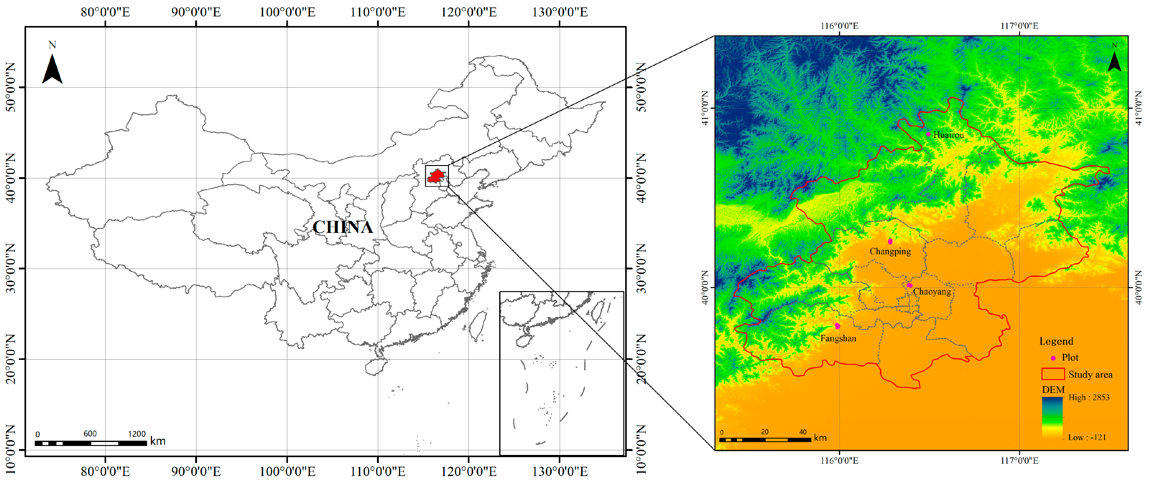
The study area was located in Beijing province (39.43°–41.05° N, 115.42°–117.50° E) (Figure 1). The long-term annual averages of minimum and maximum daily air temperatures in Beijing are 9 °C and 19 °C, respectively, with an altitude range of 20–1500 m. Ten rectangular plots, including one with dimensions of 32 m × 32 m (low stem density) and nine with dimensions of 16 m × 16 m, were used to obtain experimental data in the study; of those, 2, 2, 3 and 3 were respectively located in Chaoyang District, Huairou District, Changping District and Fangshan District. The topography of the plots was characterized by gentle slopes of less than 45 degrees. Data acquisition was carried out in coniferous, broad-leaved and mixed arbor plantations during the period from March to May of 2018. The main tree species were gingko (Ginkgo biloba), saliz matsudana (Salix matsudana), Chinese scholartree (Sophora japonica), Chinese pine (Pinus tabulaeformis), Chinese catalpa (Catalpa bungee), white wax (Fraxinus pennsylvanica), Chinese white poplar (Populus tomentosa), locust (Robinia pseudoacacia), metasequoia (Metasequoia glyptostroboides) and China savin (Juniperus chinensis), which are common trees in the boreal forests of china. The trees specimens had different bark roughness and trunk curvature. There were low shrubs in the study area, all of which were less than 1.2 m in height, that had no effect on the acquisition of DBH from the point cloud data of trunks.

2.2. Data Acquisition

2.2.1. Field Data Collection

Field surveys were conducted to collect data, including tree species, DBH and tree height information. The data was collected in ten different sampling plots using traditional forest inventory methods. An experienced taxonomist accompanied the survey team to identify the tree species in the field. The allometric growth biomass models used in this study all require DBH greater than 5 cm. Therefore, the DBH of each tree of more than 5 cm was manually measured using a diameter tape with millimeter accuracy at DBH height (1.3 m vertical above the ground from the base of the tree). A total station with centimeter-scale ranging accuracy developed by the South Surveying and Mapping Technology CO., LTD (Guangzhou, China) was used to accurately measure the tree height in the plot, which was achieved by the principle of triangulation. The structure parameters of the ten forest types based on field forest inventory are summarized in Table 1. The growth model of a specific tree species was used to estimate the tree height in cases where the treetop was not visible due to occlusion by adjacent trees (a total of 13 tree heights were calculated by the tree growth model) [30,31,32]. The DBH and tree height data of 322 trees obtained in the field were used as references, which were provided in Table S1 of Supplementary Materials.

2.2.2. TLS Data Collection

The TLS data were collected in the spring of 2018 using a FARO Focus S 150 terrestrial laser scanner produced by FARO Technologies Company (FL, America), a phase-based scanner with a field of view of 360° horizontally and approximately 300° vertically, and a minimum horizontal and vertical step size of 0.009° (approximately 40,000 laser pulses for a full hemispherical scan). The maximum rate of the laser scanner data acquisition was 976,000 points per second, and an acquisition rate of 244,000 points per second was used in this study. The scanner employed a continuous wave of 1500 nm to measure distances with a range of up to 153 m. The laser scanning level of the scanner is one level. The system’s distance error is less than 1 mm within a distance of 25 m, which helped to acquire highly accurate data for the surveyed forest sample plots. More detailed information about the device is provided in Table 2. The laser scanner device with an embedded microcomputer can store and preprocess the point cloud data after completion of data collection. The laser scanner had corresponding FARO Scene desktop software (FARO Technologies, Inc., version 7.1.0, www.faro.com) for post-processing of point cloud data. The FARO Scene software was used to assess the quality of the point cloud data and filter out “ghost points” and discrete points. Finally, by utilizing the functions of “Clear Sky” and “Clear Contour,” we obtained more reliable 3D spatial data for further modelling.
In order to reduce the effects of tree occlusion and terrestrial vegetation, we used a multi-scan (MS) approach to obtain better point cloud coverage for the 16 m × 16 m plot, setting scanning positions at four corners of the plot and the center to perform four consecutive scans of the trees in a clockwise sequence. In order to obtain similar point cloud coverage, we scanned the 32 m × 32 m plots according to the layout principle of 16 m × 16 m plots, and scanned a total of 13 positions. Six highly reflective target spheres were placed throughout the plot for registration of point cloud data at different scanning sites using Scene software, and the accuracy of registration was within 1 cm. In addition, the acquisition of all the plot scanning data was conducted at the same scan resolution to eliminate the effects of different resolution on the modeling results, and carried out under windless conditions, which helps to avoid inconsistencies in the spatial position of the same branches at different scanning locations.

2.3. Processing of the Point Cloud Data

2.3.1. Filtering

Filtering of the acquired point cloud data is the basis for accurate and precise modeling. In addition, reducing the size of point cloud data helps to save memory and reduces computation time [25,28]. First, point cloud data outside the plot area was removed. In order to obtain data for the complete canopy of the trees located at the edges of the plot, we set a 5 m buffer zone along the boundary of each plot. Any data beyond this range was excluded from further modeling. Subsequently, point cloud data that did not contain information on tree attributes in the plot was manually removed by visual inspection. Secondly, the ground points and other unrelated understory point clouds were also filtered out. We used the open source software CloudCompare (https://www.danielgm.net/cc/) to automatically filter the ground points. In addition, the height of the understory shrub vegetation in the plots was less than 1.5 m, so the shrub point cloud data in the plot was removed. Third, in order to make the volume of the reconstructed trunks more similar to the volume of the real trees, the noise and outliers were removed from the data, since these could result in the fitting of wrong cylinder models and overestimating the trunk volume [28,33]. A sphere with a radius of 0.3 cm was used to filter noise points in cloud data of plots while removing outliers. Finally, visual inspection of the point cloud data of the trees in the plot was done to manually remove the points from adjacent crowns or stems, if present [34].

2.3.2. Extracting of Individual Trees

In order to achieve accurate modeling of trees and acquisition of their structural parameters, individual trees were extracted from the acquired point cloud data of each plot. The approaches typically used to extract individual trees include fully manually, semi-automatic and automated methods [25,35,36,37]. Manual extraction of individual trees from large point clouds is inefficient and time-consuming, and it is difficult to accurately segment branches of trees in a dense forest. Therefore, a bottom-up automatic extraction algorithm of individual trees based on biological theory and metabolic ecology theory was used in this study.
The segmentation algorithm of individual trees used in the study, called comparative shortest-path (CSP), was developed by Tao et al. [37]. It is a bottom-up method based on the 3D structure of point cloud data. The extraction of individual trees from the plot was mainly composed of three parts. First, ground points were filtered and normalized. Since the plot terrain was not strictly a two-dimensional plane, ground points were separated before individual tree extraction in order to eliminate the influence of topographic fluctuation on the z-value of the point cloud data. The filtered ground points were generated using a digital elevation model (DEM) of 0.3 m resolution via Kriging interpolation, and the minimum z value of the point cloud data in each grid was used as the real ground to normalize the point cloud data in a plot area. Then, the density-based spatial clustering of applications with a noise algorithm (DBSCAN) was used for automatic identification of tree trunks in the plot, which required the definition of the minimum number of cluster points or the radius of neighboring points to determine whether a point belonged to the real trunk surface [37,38]. The point cloud data of a single trunk in the plot was segmented automatically. A 10 cm thick point cloud slice from the trunk (1.3 m vertical above the ground from the base of the tree) was used to calculate the DBH value as a seed point for the tree. Finally, the seed points and the CSP algorithm based on the metabolic ecology theory were used to segment the canopy point clouds of the trees. According to the distribution of trees in the forest, the canopy point cloud was mainly divided in three ways. For the forest plots where the sparsely distributed canopies did not intersect, the point cloud from the trunk was extended to the points of branches according to the shortest 3D Euclidean geometric distance to complete the segmentation of canopy point cloud data. For adjacent trees with the same size and canopy intersection, the shortest path distance from the point to the trunk was calculated based on biological theory, and the points were assigned to the closest respective target trunks. The remaining points were sequentially calculated one by one to determine the point cloud data of each tree. For the canopy intersection of trees with large differences in size, the distance from the point to the trunk was converted and reduced according to a power-law relationship between the branch length and the branch radius in according to metabolic ecology theory. Then, the converted distances were compared to determine the shortest distance, which yielded the target tree to which the point belonged. The target tree of each point in the point cloud was determined successively until the whole point cloud data was segmented. The conversion formula based on the power-law relationship [37] was as follows:
D i T r u n k T = D i T r u n k / D B H 2 / 3
where D i T r u n k T is the distance from the i-th point to the base of the trunk after transformation according to the power-law relationship; D i T r u n k is the biological distance from the i-th point to the base of the trunk; D B H 2 / 3 is the fixed scale. More detailed information on the algorithm can be found in Tao et al. [37].
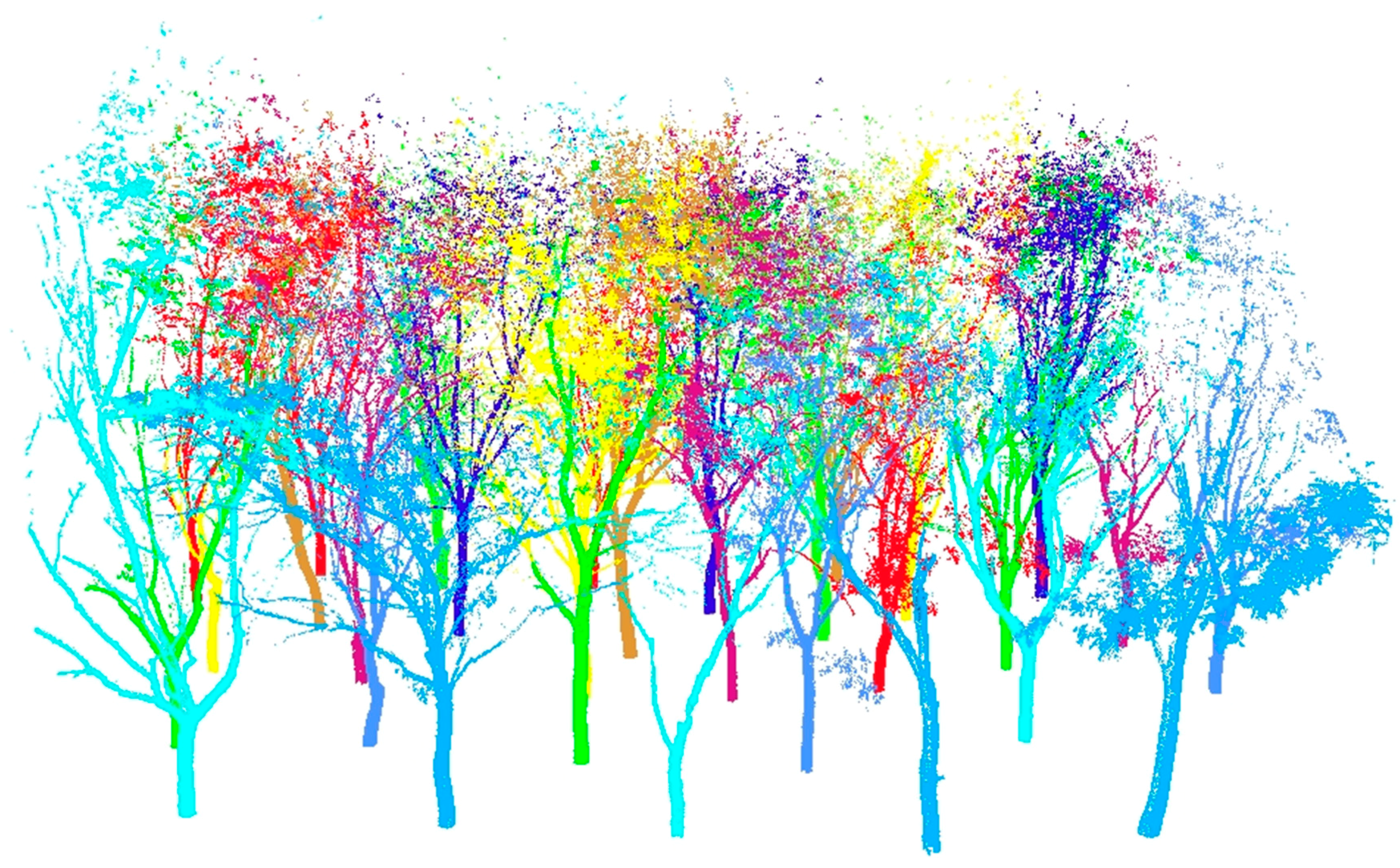
We used the segmentation algorithm to extract individual trees from 10 plots and visually inspected the results (Figure 2). The point cloud data of a single tree after segmentation was further checked one by one, and those trees that were not correctly classified were re-segmented manually, and abnormal points that did not belong to a specific tree were removed to generate more accurate point cloud data of single trees. The accuracy of single-tree segmentation directly affects the modeling results of the QSM algorithm, and thus has an impact on the estimation of aboveground biomass [3,28].

2.3.3. Acquisition of Tree Structure Parameters from TLS Data

The basic parameters of tree height and DBH were obtained from the point cloud data of the plots. The point cloud slices of 10 cm thickness (1.25 m–1.35 m) were intercepted from the filtered point cloud data, which after eliminating the effect of topographic fluctuation, and the DBH values of each tree were calculated using the least squares circle fitting method, which was considered to be the most accurate DBH estimation method compared with the least square cylinder fitting and the circle Hough transformation [3,39]. In dense forests it is difficult to measure the height of trees, because their tops are often occluded by adjacent trees. In order to obtain accurate and reliable tree height information, the top of each tree should be accurately detected by the scanner, and a sufficient number of tree vertex points should be obtained, which is about 1–2 cm in point space at the top of the tree [40]. The scanning positions of the 10 plots in this study were set up to ensure the detection of tree tops. The point cloud data of individual trees was used to calculate the tree height, which was defined as:
h t r e e = Z m a x
where h t r e e is the calculated height of a tree, while Z m a x is the maximum value of the Z coordinate in a single vertex of the tree point cloud data.
The DBH and tree height values obtained from point cloud data were also compared with those obtained from field measurements. Analysis of variance (ANOVA) was used to test whether the differences in DBH and tree height estimates were statistically significant at the 95% level of significance, and to analyze DBH and tree height, respectively [41]. The linear regression models between estimates and reference values are also used to show the differences between estimates and reference values. Precision indicators including bias, root mean squared error (RMSE), relative bias and relative RMSE (RMSE%) were used to evaluate the precision of DBH and tree height obtained from point cloud data.

2.4. Model Reconstruction and Algorithmic Optimization

2.4.1. QSM Reconstruction Method for Individual Trees

The QSM method can realize the rapid modeling of point cloud data of individual trees and accurately calculate the modelled tree volume from the reconstructed structure, including the volume of branches and the trunk. The method mainly achieved accurate tree structure reconstruction and acquisition of important structural parameters through the following eight steps. (1) The filtered point cloud data of individual tree is used for tree model reconstruction in QSM algorithm, and the corresponding cover sets are generated for the point cloud on the tree surface. (2) The neighbor- relation between the coverage sets is determined according to the size of the cover sets. (3) According to the size of the cover sets in conjunction with their eigenvalues and vectors, the local geometric features of the tree, the local directions of the trunk and branches, and the angle between the trunk and branches are determined. (4) The base of the trunk and branches are identified based on the characteristics of cover sets and the component parts of the tree are extracted by “growing”. (5) The generated cover sets of the tree surface are segmented into the corresponding real trunk and branches. (6) A series of cylinders with different radii, lengths and directions are used to conduct least-squares piecewise fitting for the point cloud data segmented in the preceding step, and the structure of each part of the tree is reconstructed. (7) The gap between the fitted cylinders are found and supplemented with cylinders to complete the cylinder model of the whole tree. (8) The volume and length of the trunk and branches are calculated automatically from the reconstructed model. The method is described and validated in detail by Raumonen et al. [28]. There are, mainly, seven parameters in the process of tree reconstruction, as follows:
t r e e _ q s m   ( d ,   r ,   n ,   d 1 ,   r 1 ,   n 1 ,   l )
where d and d 1 represent the minimum distance between the two centers of the cover sets; r and r 1 are the radii of the balls used to generate the cover sets; n and n 1 are the minimum thresholds for the number of points in a given ball; l is the ratio of the length to the radius of the fitting cylinder.
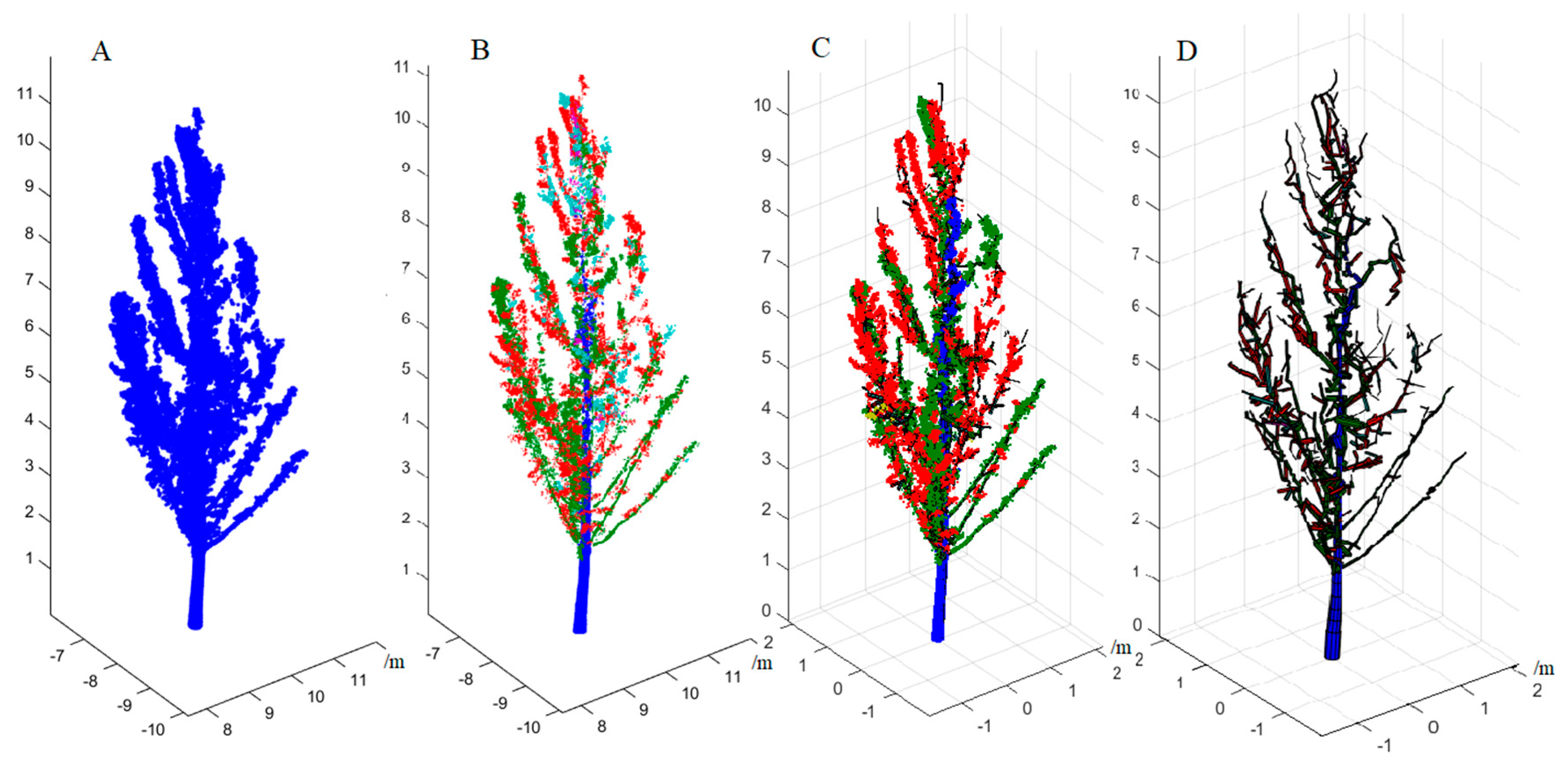
The first three parameters (d, r and n) were used to generate the first cover sets of a single tree, which primarily filters out the noise in the point cloud data for individual trees caused by small branches and leaves. The parameters d1, r1 and n1 were used to generate a finer cover, mainly to determine the neighbor-relation of the cover sets and the local characteristics of the tree. Parameter l controls the magnitude and is used to fit the cylinder. The smaller the cylinder, the more detailed the local characteristics of the tree. Figure 3 shows the point cloud data for a single specimen of Ginkgo biloba and the 3D structure reconstructed using the QSM method.

2.4.2. Optimization and Sensitivity Analysis of the QSM Algorithm

The algorithm has two important parameters, d and l, which were used to generate the reconstructed model by defining the covering sets of different sizes and the ratio of the length and radius of the cylinder, which has an important impact on the reconstruction results [3,8]. Therefore, we used different parameter values to test ten tree species with different ecological structures to determine the optimal parameters for each tree species and the sensitivity of the algorithm to different tree species with different ecological structures. Ten trees of each species were randomly selected to optimize the QSM algorithm and determine the optimal model parameters of different tree species. All the remaining data were used for the independent evaluation and precision evaluation of the estimated AGB.
We determined the optimal parameter d from different test values (2.0, 3.0, 4.0, 5.0, 6.0 and 7.0) and the optimal parameter l from different test values (3, 4, 5 and 6), which gave the most accurate biomass estimation according to Tanago et al. [8] and Raumonen et al. [28]. The other parameters r, n, d1, r1 and n1, used the default values d + 2, 3, 6, 7 and 1 cm, respectively. Firstly, the average values of the individual tree volume of the selected tree species were obtained from the 10 model realizations using different parameter values for d, after which the biomass calculated by multiplying with the basic wood density of specific tree species was compared with the biomass calculated using the regional allometric model of the same tree species. The biomass of ten trees of the tree species was calculated respectively according to this process, and the RMSE was calculated from the estimated biomass value and the reference biomass value. The optimal parameter d was determined from the corresponding parameter value with the smallest RMSE. Then, once the optimal parameter d was determined, the average value of the individual tree volume was calculated again from the 10 model realizations using different parameter values l. The biomass of the tree was calculated by multiplying its average volume by its density, and the calculated tree biomass was compared with the biomass calculated using the regional allometric model. The biomass of ten trees of the tree species was calculated respectively according to this process, and the RMSE was calculated from the estimated biomass value and the reference biomass value. The optimal parameter l was determined using the minimum RMSE. By this time, the optimal parameters d and l of a tree species were determined. The same operation was performed for the remaining tree species in turn to determine the optimal QSM algorithm for different tree species. Finally, the optimal parameters d and l of ten species were determined respectively, and the optimized QSM algorithm was used to estimate the individual tree volume of the remaining data sets and calculate the individual tree biomass via the same process as described above.
We analyzed the sensitivity of the QSM algorithm using the modeling result for different parameter values of d and l. Sensitivity analysis mainly includes two aspects: the sensitivity analysis of the QSM algorithm for different parameters of the same tree species, and the sensitivity analysis of QSM the algorithm for the same parameters of different tree species. The QSM algorithm for tree reconstruction was implemented in MATLAB software (The MathWorks, Inc., Version Matlab 2018a, Natick, MA, USA) using a Windows 10 64-bit operating system (Microsoft Corporation, Redmond, WA, USA).

2.5. Estimation of AGB

In the estimation of AGB, the differences in tree biomass caused by the errors in the measurement operation, the allometric model and the instrument itself were considered to be minimal and negligible [8,42]. Furthermore, the stem contributed about 70%–80% of the total AGB [43]. We calculated from the data released by the forestry ministerial standard of the People’s Republic of China that the biomass of the branches accounted for about 20%–30% of the total AGB. By contrast, the leaves accounted for only 10% of the total biomass, and we consequently did not consider them when assessing the AGB via the QSM method.

2.5.1. AGB Estimation from Allometric Biomass Models

The biomasses of individual trees of ten species were estimated using the regional biomass models specific for each tree species. Those biomass equations were based on variables, such as specific tree species, DBH and tree height, which were collected during the field inventory. The biomass models of the ten tree species used in this study, which evaluate the total AGB, including the biomass of the trunks, branches and leaves, were obtained from published literature and national standards or references (see Table 3). The table contains the information on the number of modelled tree species, the DBH range, tree height range, biomass model parameters, tree species density and coefficient of determination (R2). The modeling data for the tree species, including Robinia pseudoacacia, Salix matsudana, Juniperus chinensis, Sophora japonica and Fraxinus pennsylvanica, was not available in detail; therefore, only some information obtained from references is shown. The individual tree biomass obtained from these biomass models was used as a reference value and compared with the biomass calculated from the reconstructed QSM models.

2.5.2. AGB Estimation from TLS-QSM

We used point cloud data of individual trees to fit the topological structure of whole trees using cylinders via the QSM algorithm, calculated the volume of each cylinder part, and then managed to calculate the volume of the trunk and branches of each tree. For given parameters d and l, the random coverage set generated by the QSM algorithm showed small differences in the reconstruction results. Therefore, the volume of the individual tree was defined as the average volume of 10 reconstructed models. The AGB of individual trees was obtained by multiplying the volume of a specific tree (branches and trunks) by the basic wood density of the corresponding tree species. The basic wood density values of specific tree species were obtained from the Global Wood Density Database [54,55] or the literature. We calculated the RMSE, RMSE% and concordance correlation coefficient (CCC) of the biomass of the QSM model relative to the reference data to evaluate the QSM algorithm. The RMSE and RMSE% are defined in the following equations:
RMSE = 1 n ( A G B e s t i A G B r e f i ) 2 n
RMSE % = RMSE A G B r e f ¯ × 100 %
where A G B e s t i is the i-th estimation value of AGB, A G B r e f i is the ith reference value of AGB, A G B r e f ¯ is the mean of the reference AGB and n is the number of trees.

3. Results

3.1. DBH and Tree Height

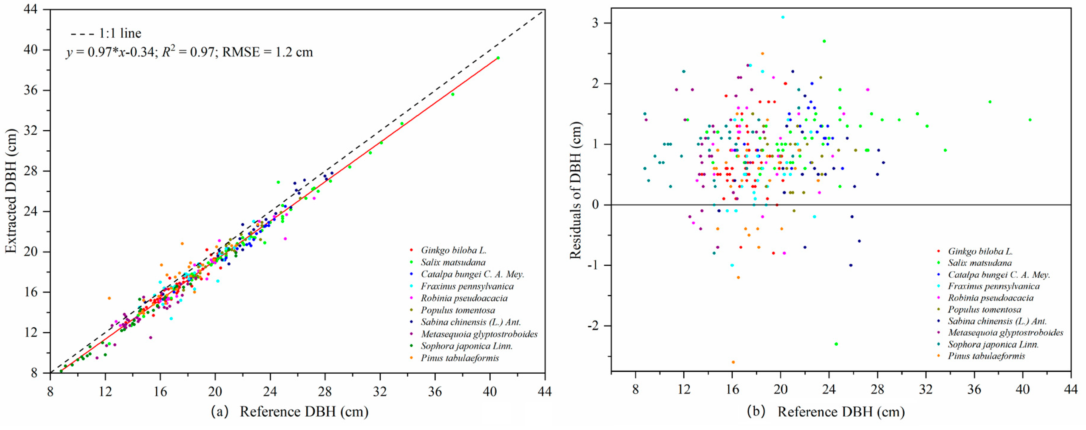
A total of 322 trees belonging to ten different species were successfully extracted without commission or omission errors. The estimated DBHs were compared with the reference DBHs, which were measured using a diameter tape (Figure 4). Our estimates showed that most of the DBHs of the ten tree species obtained from the TLS data were below the 1:1 dashed line, indicating that the DBH estimated from point cloud data was smaller than the one measured in the field (Figure 4a). The R2 of the linear regression model describing the agreement of LiDAR DBH data with the measured DBH values was 0.97, and its slope was also 0.97. A detailed analysis of the effects of different bark roughness and trunk curvature on DBH estimation for each tree species is provided in Appendix A. The underestimation of DBH from TLS data did not change significantly with the increase of DBH. As shown in Figure 4b, most of the DBH residuals of the ten tree species were above the y = 0 line, which was consistent with the result that the DBH values from TLS data in Figure 4a were smaller than the values measured in the field. There was no significant difference in the residuals of DBH among different tree species, most of which were between −0.5 cm and 2.0 cm.
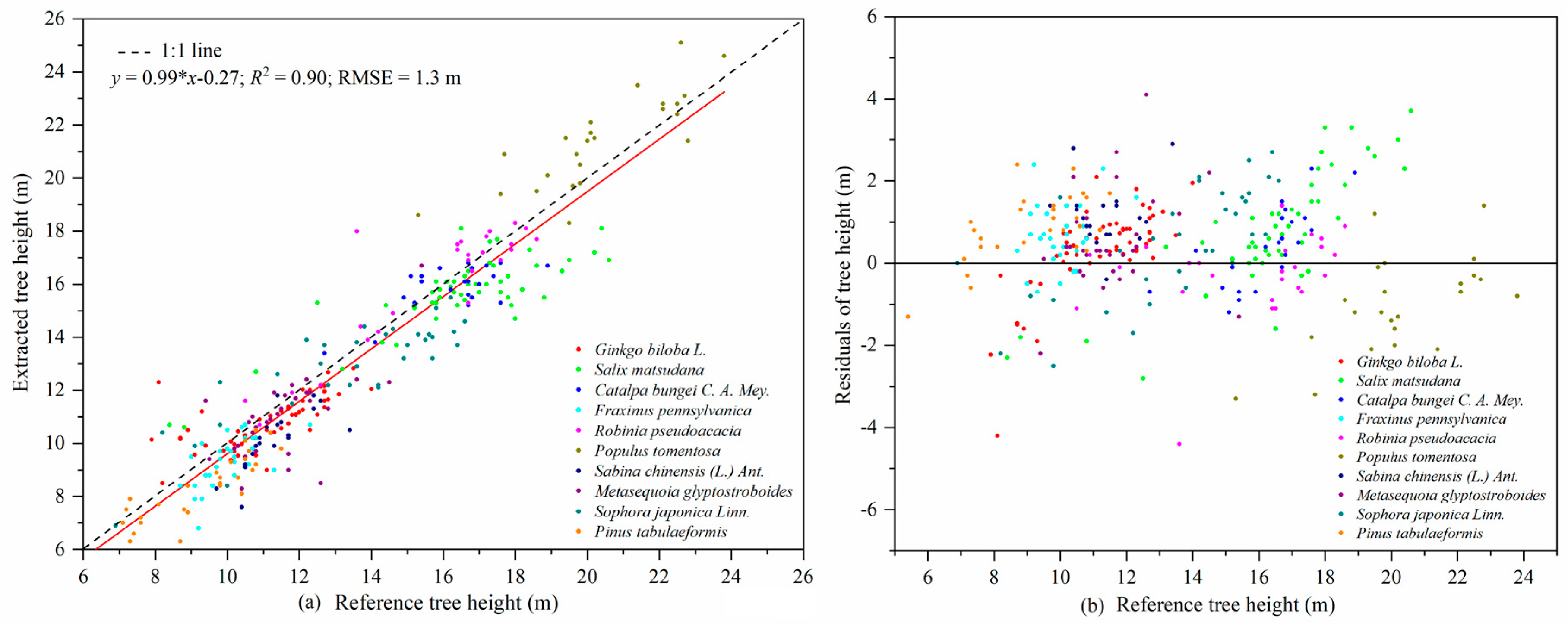
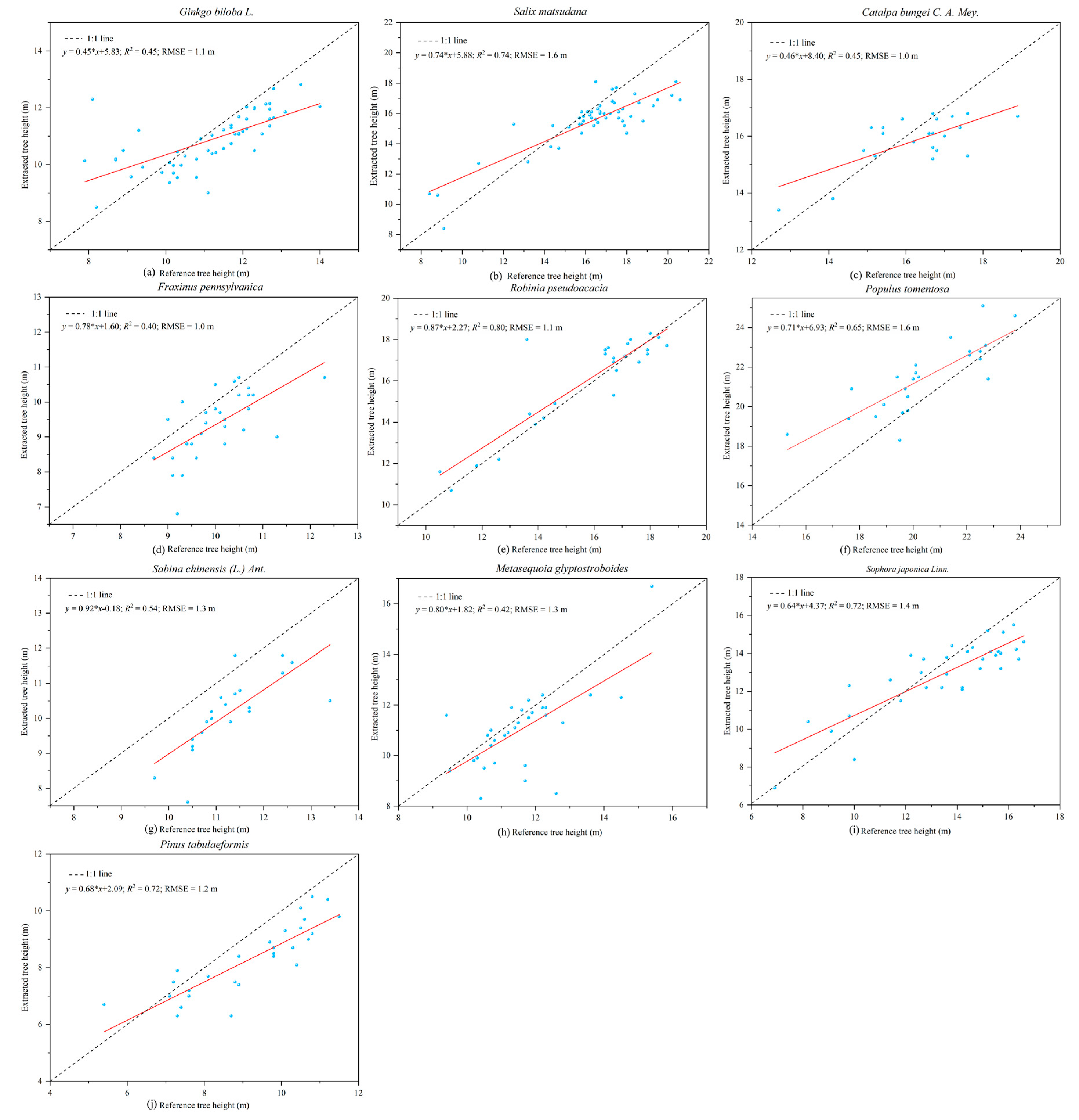
A comparison of tree heights from TLS and field measurements, with the tree height measured by the total station as a reference is shown in Figure 5. Our estimates showed that the determination coefficient (R2) of the linear regression model describing the agreement between the LiDAR tree height data and measured tree height data was 0.90, and its slope was 0.99. The tree height of Populus tomentosa estimated using the TLS data was significantly higher than that measured in situ. The estimated tree heights of Robinia pseudoacacia and Catalpa bungei were consistent with the measured values and were evenly distributed on both sides of the 1:1 line. The estimated height of other tree species was mostly lower than the measured values. A detailed analysis of the effects of different tree species on tree height estimation is provided in Appendix A. Figure 5b illustrates that the residual values of most tree heights were more uniformly distributed on both sides of the y = 0 line, and most of the residual values were between −1 m and 2 m. The tree heights obtained from point cloud data were largely underestimated compared with the heights measured in situ. No significant difference was observed in the distribution range of residual values with the increase of tree height.
The accuracy of DBH and tree height estimation using TLS data is shown in Table 4. It can be seen that the total bias and RMSE of the DBH calculated via the least square circle algorithm were −0.8 cm and 1.2 cm, respectively. Among the 322 selected trees with reference DBH values ranging from 8.8 cm to 40.6 cm, trees with a DBH bias of less than 1.5 cm accounted for 89.1% of the total. The bias and RMSE of tree heights were −0.4 m and 1.3 m, respectively. The bias of tree height from TLS data was within 1.5 m and accounted for 80.8% of the total. A more detailed analysis of tree height and DBH of different tree species is provided in Appendix A.
The analysis of variance showed that there was no statistically significant difference between the estimated DBH and tree height for all trees and the field measurements (α = 0.05; Table 5). The results of variance analysis of DBH and tree height supported the hypothesis of equality, with p-values of 0.921 and 0.056, respectively.

3.2. Optimization Parameters of the QSM Algorithm

The tree structures of different tree species were reconstructed with different parameters of d and l values, and the optimal parameters of the reconstructed model were obtained as shown in Table 6. The optimal value for parameter d was 2 or 3 cm for other tree species except for Salix matsudana, Fraxinus pennsylvanica and Pinus tabulaeformis. The minimum relative RMSE of Populus tomentosa was 7.1%, while the maximum relative RMSE of Pinus tabulaeformis was 25.6%. The optimal value of the parameter l for different tree species was evenly distributed between 3, 4 and 5, and there was no obvious difference between different forest types. The optimal l value of the algorithm had a significant effect on the reconstruction results of Ginkgo biloba, and the relative RMSE increased from 21.5% to 14.9%. For other tree species, the optimal l value had no significant effect on the accuracy of the reconstruction results. Therefore, the optimal values of these parameters for the different tree species were used to reconstruct the model of the remaining data.

3.3. Estimation of Above-Ground Biomass

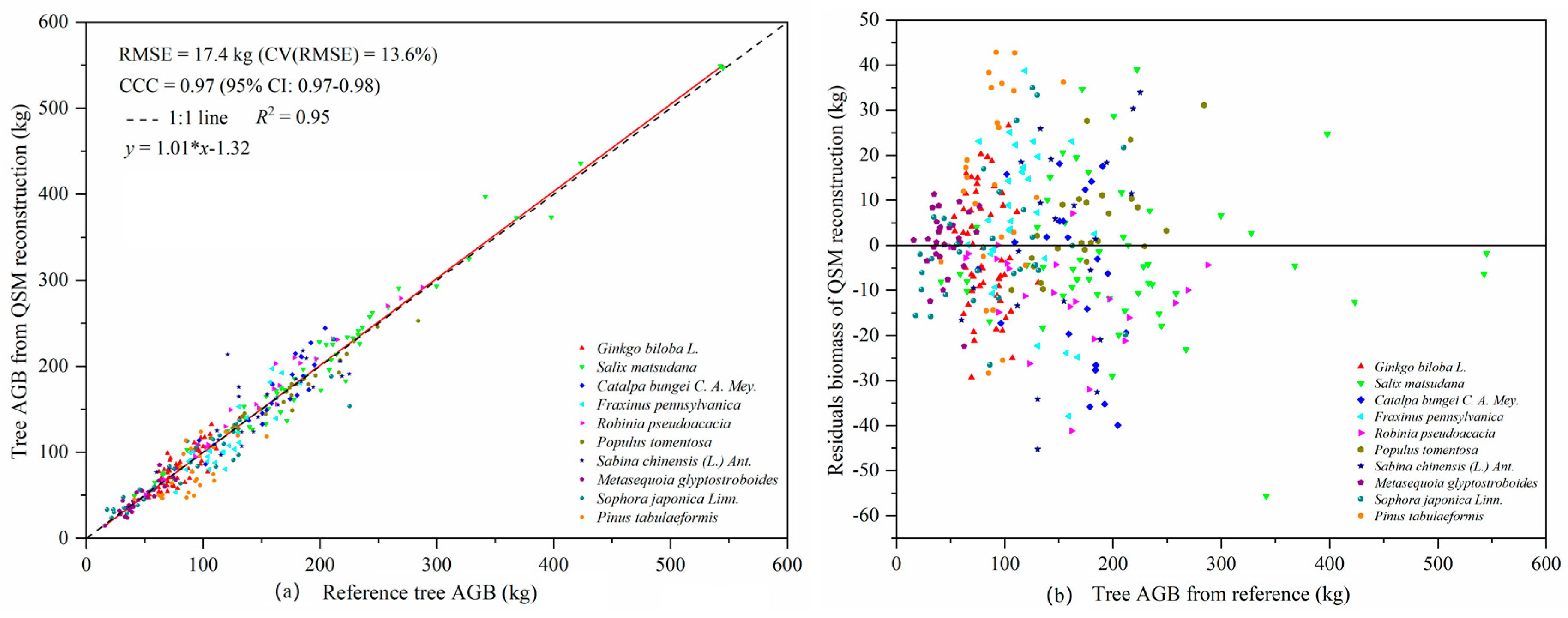
When the QSM algorithm was used to reconstruct tree structure, nine individual trees failed to model, including two Ginkgo biloba, one Salix matsudana, one Robinia pseudoacacia, two Metasequoia glyptostroboides and three Pinus tabulaeformis. Consequently, the data of these nine trees were eliminated from modeling. A comparison of the AGB of each tree from the TLS-QSM model and the basic wood density with the corresponding reference AGB is shown in Figure 6. The comparison between the AGB calculated by TLS-QSM and the AGB from the regional allometric model indicated that the total RMSE and CV (RMSE) of the AGB obtained via TLS-QSM were 17.4 kg and 13.6%, respectively. The correlation between the AGB values from TLS-QSM and the allometric model, expressed by a linear regression model, was 0.95. The TLS-QSM approach and regional allometric model were highly consistent in regard to the 95% confidence interval level (CCC = 0.97), with no major systematic deviation from the 1:1 line (slope of 1.02). Hence, there was no tendency to overestimate or underestimate the AGBs of larger trees. Figure 6b shows the distribution of the AGB residuals from different tree species. Compared with the regional allometric models, the TLS-QSM method for calculating AGB with basic density has neither systematically tended to overestimate nor underestimate the AGB of a particular tree species for different tree species.
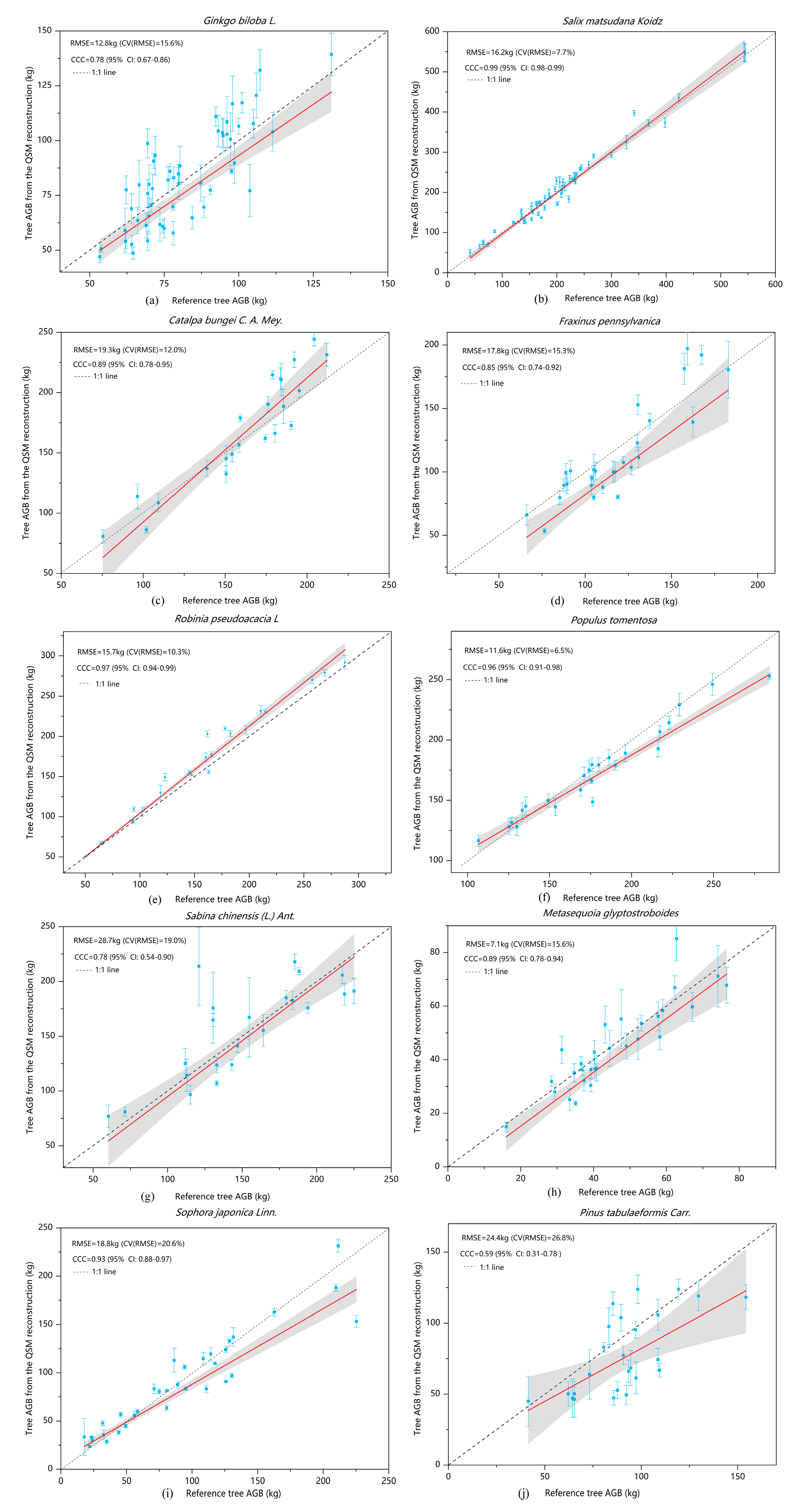
Figure 7 depicts the average modeled AGB from ten different QSMs for each tree and compares them to the reference AGB. The QSM algorithm showed significant differences in modeling accuracy and stability for tree species with different morphological and topological structural characteristics. The best AGB modeling results were achieved for Salix matsudana and Populus tomentosa, with RMSE, CV (RMSE) and CCC values of 16.2 kg and 11.6 kg, 7.7% and 6.5% and 0.99 and 0.96, respectively (Figure 7). When modeling Juniperus chinensis and Pinus tabulaeformis, we found that the branches of some of the trees were disturbed and destroyed by people. Therefore, the AGB-calculated by the model was quite different from that of the regional allometric model, and we did not conduct a more detailed analysis of those values. Ginkgo biloba showed large deviations and large uncertainties compared to other tree species. Our results showed that small trees showed lesser uncertainties and lesser deviations from the reference than large trees. The linear regression slopes of the models for Catalpa bungei and Robinia pseudoacacia were 1.17 and 1.05, respectively, indicating that the TLS-QSM approach slightly overestimated the AGBs of larger trees. By contrast, the TLS-QSM approach slightly underestimated the AGBs of the large Populus tomentosa and Sophora japonica, and the slope of their linear regression models was 0.84.
The analysis of variance showed that there was no statistically significant difference between the AGB estimates and reference values for different tree species (α = 0.05; Table 7). The results of variance analysis supported the hypothesis of equality. When the same analysis was performed for ten different tree species using the assumptions of equal AGB means, p-values were 0.895, 0.811, 0.542, 0.651, 0.559, 0.685, 0.725, 0.881, 0.787 and 0.117 for Salix matsudana, Ginkgo biloba, Catalpa bungei, Fraxinus pennsylvanica, Robinia pseudoacacia, Populus tomentosa, Juniperus chinensis, Metasequoia glyptostroboides, Sophora japonica and Pinus tabulaeformis, respectively.

3.4. Sensitivity Analysis of the QSM Algorithm

We mainly analyzed the sensitivity and stability of the QSM algorithm according to the RMSE of tree AGBs generated using different values for the parameters d and l, and the standard deviation produced by the given parameter values in the QSM algorithm for ten modeling times per tree. Table 8 and Table 9 respectively, show the differences of AGB for different tree species, calculated using different values for the parameters d and l in the QSM algorithm. The different values of d had a great influence on the volume of the trunks and branches reconstructed by the QSM algorithm, and consequently a great impact on the evaluation of AGB (Table 8). Different tree species had large errors in the reconstruction results for the same value of d, which indicated that the algorithm was impacted by the different morphological structures of different tree species. We also found that different parameter values had no significant impact on the reconstructed trunk volume, but had a great impact on the volume of the reconstructed branches. Table 9 describes the effects of different values of the parameter l on the tree AGB reconstructed by the QSM algorithm. It can be seen that different values of l had no significant impact on the reconstructed AGB of specific trees, which indicates that the parameter l of the QSM algorithm has low sensitivity and high stability for the reconstruction results.

4. Discussion

TLS is a powerful and effective tool for obtaining 3D point cloud data of the morphological structures of individual trees, and then extracting a variety of geometric and statistical parameters. The least squares circle fitting algorithm was used to fit point clouds at DBHs of trees with different bark roughness and trunk curvature. The results showed that different bark roughness and trunk curvature had a minor influence on the evaluation of DBH in laser point clouds [56,57]. The comparison of DBH from TLS data and field measurements shows a high consistency. The precision of the DBH estimation in our study (RMSE = 1.2 cm) was higher than that reported by Calders et al. [2] and Cabo et al. [58]. The slope of the fitting line between the estimated DBH and the measured data was 0.97, which indicated that the DBH of trees was slightly underestimated on the whole. In addition to the influence of bark roughness, the main reasons for the smaller DBH estimation were the shape of the trunk and the low density and uneven distribution of point cloud data [40,56]. The precision of the tree height estimation (RMSE = 1.3 m) in our study was lower than that reported by Cabo et al. [58]. That was likely due to the higher trunk density in our plots, which caused occlusion of tree tops, leading to the modelling error of the tree height-DBH model. Obtaining tree height from point cloud data has an obvious advantage over other instruments for measuring tree height since it does not rely on the artificial selection of tree vertices. This method is more advantageous for measuring tree height in dense forests where the tops of trees cannot be seen [59,60].
A QSM algorithm optimized for different tree species based on their biophysical characteristics can provide reliable and highly accurate estimates of AGB. The optimal value for the parameter d was 2 or 3 cm for all investigated tree species except Salix matsudana, Fraxinus pennsylvanica and Pinus tabulaeformis, which is consistent with the results of Calders et al. [2] and Tanago et al. [8]. The optimal value for the parameter l for different tree species was always 3, 4 or 5, which was consistent with the results of Raumonen et al. [28]. The optimum value for the parameters d and l for different trees species were obviously different, which was mainly influenced by the different biophysical and morphological structures of the trees. Different parameters of the QSM algorithm have a great impact on the final model reconstruction results. The method we used to reconstruct the model from TLS data does not require prior assumptions about tree structure, nor does it rely on limited tree structure parameters. Calders et al. [2] used the QSM algorithm to reconstruct the tree structure of Eucalyptus leucoxylon, E. microcarpa and E. tricarpa, and then evaluated the tree AGB. The results of the AGBs calculated using their TLS-QSM method were highly consistent with the reference values, with the CV (RMSE) and CCC being 16.1% and 0.98, respectively. The accuracy of the total AGB estimated using the optimized QSM algorithm in our study was higher than that reported by Calders et al. [2], and our CV (RMSE) and CCC were 13.6% and 0.97 respectively. The accuracy of the AGB estimated in our study was significantly higher than that of an estimate for 29 tropical rainforest trees species during the foliage period (CV(RMSE) = 28.37%, R2 = 0.90, CCC = 0.95) [8]. The modelled volumes of different tree species calculated using the QSM algorithm were quite different. In addition to the influence of the biophysical structure of trees, an important reason is the difference in the stem density in the sample plots populated by different species. Among of 322 trees, nine failed to model when performing the 3D reconstruction of tree structure. Possible reasons include a lack of point cloud data in some trees and problems in the algorithm itself. Because different point cloud densities will affect the results of QSM modeling, we used the same scanning resolution and set the same scanning mode and the same point cloud data processing method in ten sample plots to ensure that the single trees used for QSM model reconstruction had similar point cloud densities, which reduces the impact of different point cloud density on the modelling results. The point cloud data of Ginkgo biloba were acquired in the period of leaf growth, and the acquired data contained the point cloud data of leaves, which led to discrepancies in the cylinders fitted in the modeling of branches, and further. led to a large standard deviation in the biomass of individual modelled trees (Figure 7a). By contrast, the point cloud data of Salix matsudana and Populus tomentosa were less affected by leaves and the biophysical morphologies of the trees were relatively simple, so that the modelled results showed high consistency with the reference biomasses (Figure 7b,f). When the QSM algorithm was used to repeatedly model the same individual tree a total of 10 times, the modelled volume of the trunk was very similar, whereas the modelled volume of the branches varied greatly, up to several times. An important reason was that the point cloud that newly grows out of the leaves caused the fitted branches to be bulky. This method can not only calculate the volume and biomass of trees, but also monitor the annual natural growth of tree volume, as well as changes of branches and trunks [28]. Kaasalainen et al. [61] used this method to monitor the same tree in successive years and quantitatively evaluate its growth of tree volume.
There are many factors influencing the calculated AGBs of trees, including allometric biomass models. The allometric biomass models for a specific area have high accuracy in assessing the biomass of individual trees. Therefore, all allometric biomass models used in this study were specific for the area and tree species under investigation. In this study, the single variable (DBH) AGB prediction model was only adopted for Juniperus chinensis, and the two variable (DBH and tree height) AGB prediction model, which has higher accuracy of biomass assessment [62], was used for all the other tree species. There are three main reasons for the inconsistency of the biomass calculated by the QSM algorithm using basic wood density and regional allometric biomass models. First, the model data of the regional allometric biomass equations of different tree species are inconsistent, which lead to differences of model accuracy and inevitable systematic errors of the model itself, all of which had an impact on the final biomass results for specific trees. Secondly, there is sensitivity and instability of the QSM algorithm in the process of volume reconstruction of individual trees and the influence of the differences of basic wood density on the calculation of the AGB of trees. Thirdly, we did not consider the biomass of leaves in this study, because we found that it accounts for only a small part (about 10%) of the total AGB, but it also directly affected the calculated AGBs of trees. In addition, dead branches, lack of branches, incomplete extraction of a tree’s point cloud and other factors also lead to differences between the calculated AGBs of trees reconstructed using the QSM algorithm and the biomasses calculated by the model.
We optimized the reconstruction process of the QSM algorithm based on parameters d and l, which have the most influence on the reconstruction results [2]. The results showed that the optimum values of parameter d from most of the ten tree species was 2 or 3 cm, which s consistent with the results of Raumonen et al. [28,63]. For different tree species, the optimal QSM algorithm had obvious differences. At the same time, the influence of the parameter l on the modeling results was not very significant. This provides an important reference for researchers who use the QSM algorithm for other research. The QSM algorithm should further implement the automatic determination of the optimal parameters of different tree species in the process of structural reconstruction and the automatic output of the average values of multiple modeling realization as the final result to improve the accuracy of wood volume and biomass assessment.
Future research will focus on more accurate estimation of tree volume and biomass from point cloud data and how to use non-destructive approaches to replace the destructive felling of trees to create and correct new allometric biomass models for specific tree species, especially for large trees.
5. Conclusions

We quantitatively analyzed the effects of different bark roughness and trunk curvature on DBH estimation, and the results indicated that neither parameter had a severe impact. The TLS-QSM method optimized in our study can be used to accurately evaluate the AGB of trees with different morphological and topological structures from 3D reconstructed data, which compared with the reference AGB from specific allometric biomass models. However, since we did not harvest trees in this study, the AGB estimated from TLS data was not compared to the actual value of biomass. The results of this study show that our optimized approach can provide a potential possibility for the development and calibration of allometric biomass models, especially for large trees and precious tree species that are not usually harvested and measured. Using our optimized QSM algorithm, we can continuously monitor different trees to evaluate their growth, health, economic value and ecological benefits. In addition, we can also analyze more potential information in a given forest structure based on the model reconstructed by our optimized algorithm, including the height under the first branch, the height of the tree crown, tree crown shape, crown volume and so on.

Supplementary Materials

The following are available online at https://www.mdpi.com/1999-4907/10/11/936/s1, Table S1: Original Data.

Author Contributions

Conceptualization, S.C. and Z.F.; methodology, S.C.; validation, S.C. and P.C.; formal analysis, S.C. and T.U.K.; investigation, S.C., P.C. and Y.L.; writing—original draft preparation, S.C.; writing—review and editing, S.C. and T.U.K.; proof reading, T.U.K. and P.C.

Funding

This research was funded by the Fundamental Research Funds for the Central Universities (grant number 2015ZCQ-LX-01), the National Natural Science Foundation of China (grant number U1710123).

Acknowledgments

The authors wish to say thanks to J.S., Y.F., and Z.Z., for helping with collecting data.

Conflicts of Interest

The authors declare no conflict of interest.

Appendix A

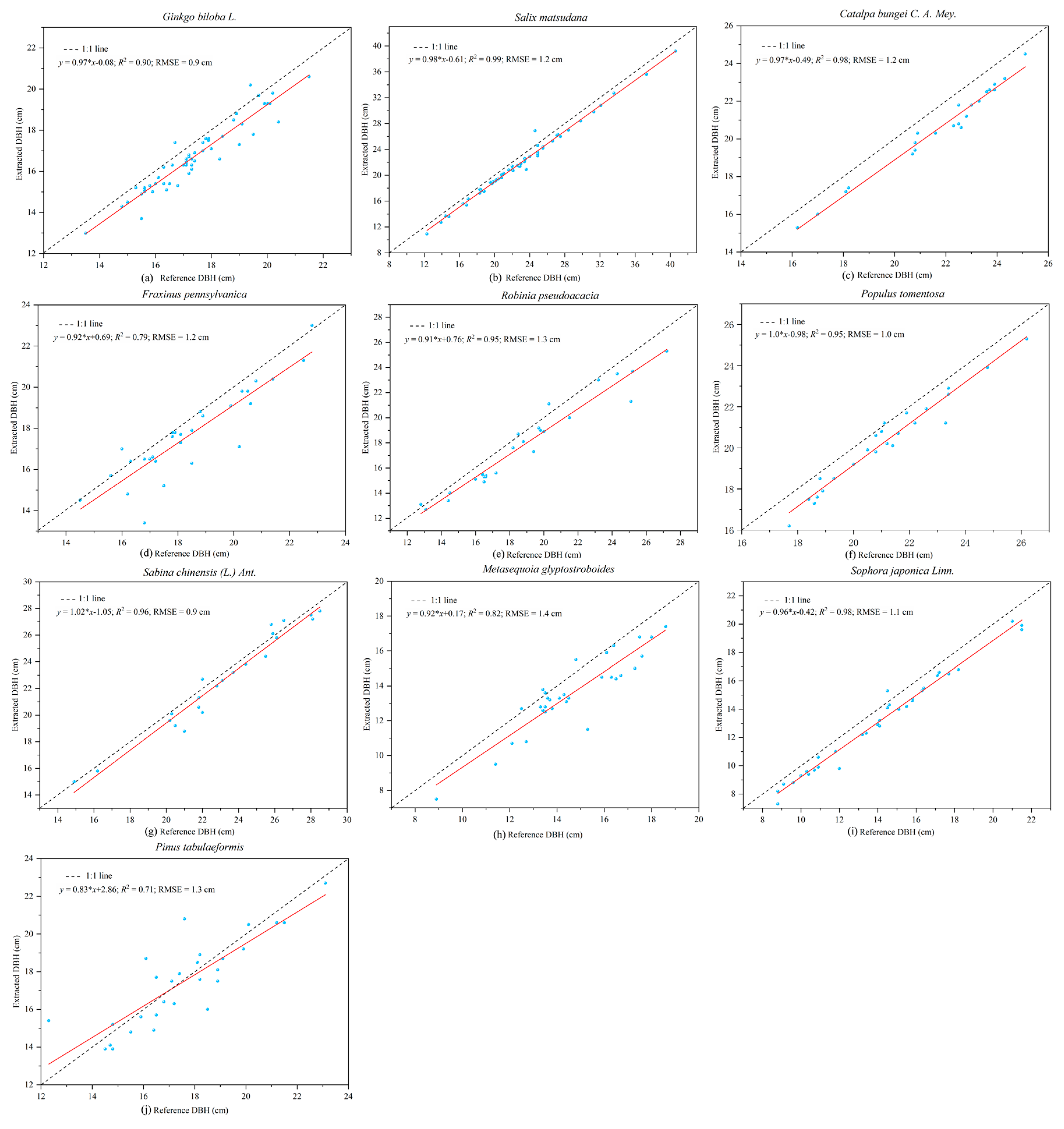
The least squares circle fitting algorithm was used to fit the DBHs of 10 cm thick slices of trees with different bark roughness and trunk curves. The estimated DBH from TLS point cloud data was compared with the measured DBHs, as shown in Figure A1. The estimated DBHs and reference DBHs of different tree species showed a good linear fit. Bark roughness of ten tree species was measured using a method similar to that of Sioma et al. [64]. Finally, we classified Salix matsudana, Robinia pseudoacacia, Metasequoia glyptostroboides and Pinus tabulaeformis into the rough bark group; Catalpa bungei, Fraxinus pennsylvanica, Sabina chinensis and Sophora japonica into the moderately rough bark group; and Ginkgo biloba and Populus tomentosa into the smooth bark group. Analysis of variance (ANOVA) was used to test whether the differences between estimates and reference values of DBH for different tree species were statistically significant at the 95% level of significance. As can be seen from Figure A1 and Table A1, the DBHs of the ten tree species from LiDAR point cloud data were underestimated to different extents compared with the measured DBH. The DBH of the same tree species was not overestimated with the increase of DBH. The RMSEs of Ginkgo biloba in the smooth bark group and Juniperus chinensis in the moderately rough bark group were the smallest, both of which were 0.9 cm. The RMSE of the moderately rough bark group was mostly 1.2 cm. The assessment accuracy of Metasequoia glyptostroboides, Robinia pseudoacacia and Pinus tabulaeformis in the rough bark group was the lowest, with RMSE values of 1.4, 1.3, and 1.3 cm, respectively. Therefore, we could infer that the assessment accuracy of the DBH decreased gradually with the increase of bark roughness, which indicated that DBH assessment from laser point cloud data would be affected by bark roughness. However, the accuracy of DBH evaluation of different species with different bark roughness was not very different.
Figure A1. Comparison of DBH calculated for tree species with different bark roughness and trunk curvature with measured DBH (aj stands for the different tree species).
Forests 10 00936 g0a1
The accuracy of the DBH estimation for ten different tree species utilizing TLS data is shown in Table A1. It can be seen that all deviations are less than zero, which indicates that all the calculated DBH values were underestimated compared with the measured DBH. Catalpa bungei had the largest bias of −1.2 cm and a relative bias of −5.4%. The bias of Pinus tabulaeformis was the smallest, at −0.1 cm, and the relative bias was −0.4%. The RMSE of DBH values of the ten tree species ranged from 0.9 cm to 1.4 cm, which indicates that the differences between species were not very large. The RMSE values of Metasequoia glyptostroboides, Robinia pseudoacacia and Pinus tabulaeformis were large, at 1.4, 1.3 and 1.3 cm, respectively, and the corresponding relative RMSE values were 9.6%, 7.0% and 7.4%. The RMSE values of Ginkgo biloba and Juniperus chinensis were the smallest, both at 0.9 cm, and the relative RMSE values were 4.9%, and 3.9% respectively, which was consistent with the preceding results.
Table A1. The accuracy of the DBH estimations for ten different tree species utilizing TLS data.
SpeciesBias (cm)Bias%RMSE (cm)RMSE%
Salix matsudana−1.1−4.61.25.3
Ginkgo biloba−0.7−3.90.94.9
Catalpa bungei−1.2−5.41.25.6
Fraxinus pennsylvanica−0.7−4.01.26.6
Robinia pseudoacacia−1.0−5.31.37.0
Populus tomentosa−0.8−3.91.04.5
Juniperus chinensis−0.5−2.20.93.9
Metasequoia glyptostroboides−1.1−7.31.49.6
Sophora japonica−0.9−6.71.17.6
Pinus tabulaeformis−0.1−0.41.37.4
The analysis of variance showed that there was no statistically significant difference between the DBH estimates and reference values of other tree species except Ginkgo biloba (α = 0.05; Table A2). The ANOVA results of the DBH of Ginkgo biloba trees rejected the assumption of equal DBH mean (p-value = 0.037 < 0.05), and the results of ANOVA of other tree species supported this hypothesis. When the same analysis was performed for other tree species using the assumptions of equal DBH means, p-values were 0.337, 0.081, 0.185, 0.372, 0.198, 0.608, 0.052, 0.278 and 0.941 for Salix matsudana, Catalpa bungei, Fraxinus pennsylvanica, Robinia pseudoacacia, Populus tomentosa, Juniperus chinensis, Metasequoia glyptostroboides, Sophora japonica and Pinus tabulaeformis, respectively.
Table A2. The results of ANOVA analysis for DBH estimations for different tree species with degrees of freedom (DF), mean squared errors (MSs), F-values and p-values.
SpeciesDFMSF-Valuep-Value
Salix matsudana128.80.9320.337
Ginkgo biloba112.44.4750.037
Catalpa bungei114.63.2030.081
Fraxinus pennsylvanica18.31.8000.185
Robinia pseudoacacia111.60.8140.372
Populus tomentosa18.41.7060.198
Juniperus chinensis13.60.2680.608
Metasequoia glyptostroboides116.93.9310.052
Sophora japonica113.61.1990.278
Pinus tabulaeformis100.0050.941
A comparison of tree heights calculated from laser point clouds with measured tree heights for different tree species is shown in Figure A2. We can see that there are obvious differences in tree height comparisons among different tree species. The tree height of all species except Populus tomentosa was underestimated to different extents. The reference tree height was obtained using the total station, and the tree height was calculated using the growth model of the specific tree species in the specific area where the tree top was not visible. Therefore, the measured tree height in the field was close to that measured in a destructive way. The slopes of linear fitting for Ginkgo biloba, Salix matsudana, Catalpa bungei, Sophora japonica and Pinus tabulaeformis were all less than 0.70, whereby the heights of large trees were overestimated and those of small trees were underestimated. A likely reason for this is the occlusion of small trees by nearby large trees, especially in forest types with high tree density, which leads to the mistake of dividing a portion of the large trees into small trees, so that the height of the small trees is overestimated. In the case of large trees, due to the occlusion by lower trees and branches preventing the acquisition of sufficient point cloud data in the top part of the tree, there is a subsequent underestimation of tree height. As shown in Figure A2 and Table A3, there was no significant difference in the tree height estimated using TLS point cloud data between coniferous and broad-leaved forests. The estimation accuracies of the tree heights of Salix matsudana and Populus tomentosa were the lowest, with an RMSE of 1.6 m in both cases, and relative the RMSEs of 9.8%, and 7.7%, respectively. The tree height estimation accuracies of Catalpa bungei and Fraxinus pennsylvanica were the highest, with RMSE 1.0 m in both cases, and relative RMSEs of 6.3%, and 9.9%, respectively.
Figure A2. Comparison of tree heights calculated from LiDAR point cloud data of different tree species with measured tree heights (aj stand for different tree species).
Forests 10 00936 g0a2
Table A3. The accuracy of the tree height estimation for ten different tree species utilizing TLS data.
SpeciesBias (m)Bias%RMSE (m)RMSE%
Salix matsudana−0.8−4.91.69.8
Ginkgo biloba−0.3−2.71.19.8
Catalpa bungei−0.4−2.71.06.3
Fraxinus pennsylvanica−0.7−6.51.09.9
Robinia pseudoacacia0.31.81.16.9
Populus tomentosa1.15.21.67.7
Juniperus chinensis−1.1−10.01.311.7
Metasequoia glyptostroboides−0.5−4.71.311.3
Sophora japonica−0.5−3.91.410.7
Pinus tabulaeformis−0.9−9.61.213.0

References

  1. Whitehead, D. Forests as carbon sinks—benefits and consequences. Tree Physiol. 2011, 31, 893–902. [Google Scholar] [CrossRef] [PubMed]
  2. Calders, K.; Newnham, G.; Burt, A.; Murphy, S.; Raumonen, P.; Herold, M.; Culvenor, D.; Avitabile, V.; Disney, M.; Armston, J.; et al. Nondestructive estimates of above-ground biomass using terrestrial laser scanning. Methods Ecol. Evol. 2015, 6, 198–208. [Google Scholar] [CrossRef]
  3. Calders, K.; Burt, A.; Newnham, G.; Disney, M.; Murphy, S.; Raumonen, P.; Herold, M.; Culvenor, D.; Armston, J.; Avitabile, V.; et al. Reducing uncertainties in above-ground biomass estimates using terrestrial laser scanning. In Proceedings of the 2015 Silvilaser, La Grande Motte, France, 28–30 September 2015; pp. 197–199. [Google Scholar]
  4. Sarker, L.R.; Nichol, J.E. Improved forest biomass estimates using ALOS AVNIR-2 texture indices. Remote Sens. Environ. 2011, 115, 968–977. [Google Scholar] [CrossRef]
  5. Gleason, C.J.; Im, J. Forest biomass estimation from airborne LiDAR data using machine learning approaches. Remote Sens. Environ. 2012, 125, 80–91. [Google Scholar] [CrossRef]
  6. Disney, M.; Boni Vicari, M.; Burt, A.; Calders, K.; Lewis, S.L.; Raumonen, P.; Wilkes, P. Weighing trees with lasers: Advances, challenges and opportunities. Interface Focus 2018, 8, 20170048. [Google Scholar] [CrossRef]
  7. Clark, D.B.; Kellner, J.R. Tropical forest biomass estimation and the fallacy of misplaced concreteness. J. Veg. Sci. 2012, 23, 1191–1196. [Google Scholar] [CrossRef]
  8. Gonzalez de Tanago, J.; Lau, A.; Bartholomeus, H.; Herold, M.; Avitabile, V.; Raumonen, P.; Martius, C.; Goodman, R.C.; Disney, M.; Manuri, S.; et al. Estimation of above-ground biomass of large tropical trees with terrestrial LiDAR. Methods Ecol. Evol. 2018, 9, 223–234. [Google Scholar] [CrossRef]
  9. Prado-Junior, J.A.; Schiavini, I.; Vale, V.S.; Arantes, C.S.; van der Sande, M.T.; Lohbeck, M.; Poorter, L. Conservative species drive biomass productivity in tropical dry forests. J. Ecol. 2016, 104, 817–827. [Google Scholar] [CrossRef] [Green Version]
  10. Gourlet-Fleury, S.; Rossi, V.; Rejou-Mechain, M.; Freycon, V.; Fayolle, A.; Saint-André, L.; Cornu, G.; Gérard, J.; Sarrailh, J.-M.; Flores, O.; et al. Environmental filtering of dense-wooded species controls above-ground biomass stored in African moist forests. J. Ecol. 2011, 99, 981–990. [Google Scholar] [CrossRef]
  11. Calders, K.; Newnham, G.; Herold, M.; Murphy, S.; Culvenor, D.; Raumonen, P.; Burt, A.; Armston, J.; Avitabile, V.; Disney, M. Estimating above ground biomass from terrestrial laser scanning in Australian Eucalypt Open Forest. In Proceedings of the SilviLaser 2013, Beijing, China, 9–11 October 2013. [Google Scholar]
  12. Muscarella, R.; Kolyaie, S.; Morton, D.C.; Zimmerman, J.K.; Uriarte, M. Effects of topography on tropical forest structure depend on climate context. J. Ecol. 2019, 00, 1–15. [Google Scholar] [CrossRef]
  13. Soenen, S.A.; Peddle, D.R.; Hall, R.J.; Coburn, C.A.; Hall, F.G. Estimating aboveground forest biomass from canopy reflectance model inversion in mountainous terrain. Remote Sens. Environ. 2010, 114, 1325–1337. [Google Scholar] [CrossRef]
  14. Barber, D.; Mills, J.; Smith-Voysey, S. Geometric validation of a ground-based mobile laser scanning system. ISPRS J. Photogramm. Remote Sens. 2008, 63, 128–141. [Google Scholar] [CrossRef]
  15. Pu, S.; Rutzinger, M.; Vosselman, G.; Oude Elberink, S. Recognizing basic structures from mobile laser scanning data for road inventory studies. ISPRS J. Photogramm. Remote Sens. 2011, 66, S28–S39. [Google Scholar] [CrossRef]
  16. Chen, S.; Liu, H.; Feng, Z.; Shen, C.; Chen, P. Applicability of personal laser scanning in forestry inventory. PLoS ONE 2019, 14, e0211392. [Google Scholar] [CrossRef]
  17. Ene, L.; Næsset, E.; Gobakken, T.; Mauya, E.; Bollandsås, O.; Gregoire, T.G.; Ståhl, G.; Zahabu, E. Large-scale estimation of aboveground biomass in miombo woodlands using airborne laser scanning and national forest inventory data. Remote Sens. Environ. 2016, 186, 626–636. [Google Scholar] [CrossRef]
  18. Næsset, E.; Ørka, H.O.; Solberg, S.; Bollandsås, O.M.; Hansen, E.H.; Mauya, E.; Zahabu, E.; Malimbwi, R.; Chamuya, N.; Olsson, H.; et al. Mapping and estimating forest area and aboveground biomass in miombo woodlands in Tanzania using data from airborne laser scanning, TanDEM-X, RapidEye, and global forest maps: A comparison of estimated precision. Remote Sens. Environ. 2016, 175, 282–300. [Google Scholar] [CrossRef]
  19. Tymen, B.; Réjou-Méchain, M.; Dalling, J.W.; Fauset, S.; Feldpausch, T.R.; Norden, N.; Phillips, O.L.; Turner, B.L.; Viers, J.; Chave, J. Evidence for arrested succession in a liana-infested Amazonian forest. J. Ecol. 2016, 104, 149–159. [Google Scholar] [CrossRef]
  20. Edrisi, S.A.; Abhilash, P.C. Sustainable bioenergy production from woody biomass: Prospects and promises. J. Clean. Prod. 2015, 102, 558–559. [Google Scholar] [CrossRef]
  21. Skowronski, N.S.; Clark, K.L.; Gallagher, M.; Birdsey, R.A.; Hom, J.L. Airborne laser scanner-assisted estimation of aboveground biomass change in a temperate oak–pine forest. Remote Sens. Environ. 2014, 151, 166–174. [Google Scholar] [CrossRef]
  22. Cao, L.; Gao, S.; Li, P.; Yun, T.; Shen, X.; Ruan, H. Aboveground Biomass Estimation of Individual Trees in a Coastal Planted Forest Using Full-Waveform Airborne Laser Scanning Data. Remote Sens. 2016, 8, 729. [Google Scholar] [CrossRef]
  23. Kukko, A.; Kaijaluoto, R.; Kaartinen, H.; Lehtola, V.V.; Jaakkola, A.; Hyyppä, J. Graph SLAM correction for single scanner MLS forest data under boreal forest canopy. ISPRS J. Photogramm. Remote Sens. 2017, 132, 199–209. [Google Scholar] [CrossRef]
  24. Wang, Y.; Pyörälä, J.; Liang, X.; Lehtomäki, M.; Kukko, A.; Yu, X.; Kaartinen, H.; Hyyppä, J. In situ biomass estimation at tree and plot levels: What did data record and what did algorithms derive from terrestrial and aerial point clouds in boreal forest. Remote Sens. Environ. 2019, 232, 111309. [Google Scholar] [CrossRef]
  25. Raumonen, P.; Casella, E.; Calders, K.; Murphy, S.; Åkerblom, M.; Kaasalainen, M. Massive-Scale Tree Modelling from TLS Data. ISPRS Ann. Photogramm. Remote Sens. Spatial Inf. Sci. 2015, II-3/W4, 189–196. [Google Scholar] [CrossRef]
  26. Yao, T.; Yang, X.; Zhao, F.; Wang, Z.; Zhang, Q.; Jupp, D.; Lovell, J.; Culvenor, D.; Newnham, G.; Ni-Meister, W.; et al. Measuring forest structure and biomass in New England forest stands using Echidna ground-based lidar. Remote Sens. Environ. 2011, 115, 2965–2974. [Google Scholar] [CrossRef]
  27. Seidel, D.; Albert, K.; Ammer, C.; Fehrmann, L.; Kleinn, C. Using terrestrial laser scanning to support biomass estimation in densely stocked young tree plantations. Int. J. Remote Sens. 2013, 34, 8699–8709. [Google Scholar] [CrossRef]
  28. Raumonen, P.; Kaasalainen, M.; Åkerblom, M.; Kaasalainen, S.; Kaartinen, H.; Vastaranta, M.; Holopainen, M.; Disney, M.; Lewis, P. Fast Automatic Precision Tree Models from Terrestrial Laser Scanner Data. Remote Sens. 2013, 5, 491–520. [Google Scholar] [CrossRef] [Green Version]
  29. Momo Takoudjou, S.; Ploton, P.; Sonké, B.; Hackenberg, J.; Griffon, S.; de Coligny, F.; Kamdem, N.G.; Libalah, M.; Mofack, G., II; Le Moguédec, G.; et al. Using terrestrial laser scanning data to estimate large tropical trees biomass and calibrate allometric models: A comparison with traditional destructive approach. Methods Ecol. Evol. 2018, 9, 905–916. [Google Scholar] [CrossRef]
  30. Wu, B.; Yan, Q.; Chi, M.; Zhang, H. Harvest evaluation model and system of fast-growing and high-yield poplar plantation. Math. Comput. Model. 2010, 51, 1444–1452. [Google Scholar] [CrossRef]
  31. Liu, M.; Feng, Z.; Zhang, Z.; Ma, C.; Wang, M.; Lian, B.-L.; Sun, R.; Zhang, L. Development and evaluation of height diameter at breast models for native Chinese Metasequoia. PLoS ONE 2017, 12, e0182170. [Google Scholar] [CrossRef]
  32. Gao, X.; Xing, Z. Study on Relation of Diameter at Breast Height and Height of Sophora japonica in Liaocheng City. North. Hortic. 2010, 10, 128–130. (In Chinese) [Google Scholar]
  33. Torresan, C.; Chiavetta, U.; Hackenberg, J. Applying quantitative structure models to plot-based terrestrial laser data to assess dendrometric parameters in dense mixed forests. For. Syst. 2018, 27, 4. [Google Scholar] [CrossRef]
  34. Srinivasan, S.; Popescu, S.C.; Eriksson, M.; Sheridan, R.D.; Ku, N.-W. Multi-temporal terrestrial laser scanning for modeling tree biomass change. For. Ecol. Manag. 2014, 318, 304–317. [Google Scholar] [CrossRef]
  35. Li, W.; Guo, Q.; Jakubowski, M.K.; Kelly, M. A New Method for Segmenting Individual Trees from the Lidar Point Cloud. Photogramm. Eng. Rem. Sens. 2012, 78, 75–84. [Google Scholar] [CrossRef] [Green Version]
  36. Lu, X.; Guo, Q.; Li, W.; Flanagan, J. A bottom-up approach to segment individual deciduous trees using leaf-off lidar point cloud data. ISPRS J. Photogramm. Remote Sens. 2014, 94, 1–12. [Google Scholar] [CrossRef]
  37. Tao, S.; Wu, F.; Guo, Q.; Wang, Y.; Li, W.; Xue, B.; Hu, X.; Li, P.; Tian, D.; Li, C.; et al. Segmenting tree crowns from terrestrial and mobile LiDAR data by exploring ecological theories. ISPRS J. Photogramm. Remote Sens. 2015, 110, 66–76. [Google Scholar] [CrossRef] [Green Version]
  38. Wu, J.; Cawse-Nicholson, K.; van Aardt, J. 3D Tree Reconstruction from Simulated Small Footprint Waveform Lidar. Photogramm. Eng. Rem. Sens. 2013, 79, 1147–1157. [Google Scholar] [CrossRef]
  39. Tansey, K.; Selmes, N.; Anstee, A.; Tate, N.J.; Denniss, A. Estimating tree and stand variables in a Corsican Pine woodland from terrestrial laser scanner data. Int. J. Remote Sens. 2009, 30, 5195–5209. [Google Scholar] [CrossRef]
  40. Liang, X.; Kankare, V.; Hyyppä, J.; Wang, Y.; Kukko, A.; Haggrén, H.; Yu, X.; Kaartinen, H.; Jaakkola, A.; Guan, F. Terrestrial laser scanning in forest inventories. ISPRS J. Photogramm. Remote Sens. 2016, 115, 63–77. [Google Scholar] [CrossRef]
  41. Luoma, V.; Saarinen, N.; Wulder, M.A.; White, J.C.; Vastaranta, M.; Holopainen, M.; Hyyppä, J. Assessing Precision in Conventional Field Measurements of Individual Tree Attributes. Forests 2017, 8, 38. [Google Scholar] [CrossRef]
  42. Berger, A.; Gschwantner, T.; Mcroberts, R.E.; Schadauer, K. Effects of Measurement Errors on Individual Tree Stem Volume Estimates for the Austrian National Forest Inventory. For. Sci. 2014, 60, 14–24. [Google Scholar] [CrossRef]
  43. Zeng, W.S.; Tang, S.Z. A New General Allometric Biomass Model; Nature Publishing Group: London, UK, 2011. [Google Scholar]
  44. State Forestry Administration of China (SFAC). Tree Biomass Models and Related Parameters to Carbon Accounting for Pinus tabulaeformis; China Standard Press: Beijing, China, 2015. [Google Scholar]
  45. Zeng, W.-S. Developing Tree Biomass Models for Eight Major Tree Species in China. In Biomass Volume Estimation and Valorization for Energy; Jaya, S.T., Ed.; Books on Demand: Pasig City, Philippines, 2017; pp. 3–21. [Google Scholar] [CrossRef]
  46. Xiaver, B. Allometric Estimation of the Aboveground Biomass and Carbon in Metasequoia glyptostroboide Plantations in Shanghai; Cranfield University: Bedfordshire, UK, 2009. [Google Scholar]
  47. Zhuang, H.; Becuwe, X.; Xiao, C.; Wang, Y.; Wang, H.; Yin, S.; Liu, C. Allometric Equation-Based Estimation of Biomass Carbon Sequestration in Metasequoia glyptostroboides Plantations in Chongming Island, Shanghai. J. Shanghai Jiaotong Univ. 2012, 30, 48–55. (In Chinese) [Google Scholar]
  48. Liu, K.; Cao, L.; Wang, G.; Cao, F. Biomass allocation patterns and allometric models of Ginkgo biloba. J. Beijing For. Univ. 2017, 39, 12–20. (In Chinese) [Google Scholar]
  49. Zhang, X. Study on the Aboveground Biomass of the Deciduous Trees in Yanqing, Beijin. For. Sci. Technol. 2012, 37, 1. (In Chinese) [Google Scholar]
  50. Zhou, G.; Yin, G.; Tang, X.; Wang, W. China’s Forest Ecosystem Carbon Storage-Biomass Equation; Science Press: Beijing, China, 2018; pp. 40–80. (In Chinese) [Google Scholar]
  51. State Forestry Administration of China (SFAC). Tree Biomass Models and Related Parameters to Carbon Accounting for Cunninghamia Lanceolata; China Standard Press: Beijing, China, 2014. [Google Scholar]
  52. Wang, X. Research on Biomass Model of Sophora japonica Linn in Beijing; Beijing Forestry University: Beijing, China, 2011. (In Chinese) [Google Scholar]
  53. Li, H.; Lei, Y. Estimation and Evaluation of Forest Biomass Carbon Storage in China; China Forestry Publishing House: Beijing, China, 2010; pp. 52–58. (In Chinese) [Google Scholar]
  54. Jerome, C.; David, C.; Steven, J.; Lewis, S.L.; Swenson, N.G.; Zanne, A.E. Towards a worldwide wood economics spectrum. Ecol. Lett. 2010, 12, 351–366. [Google Scholar]
  55. Zanne, A.E.; Lopez-Gonzalez, G.; Coomes, D.A.; Ilic, J.; Jansen, S.; Lewis, S.L.; Miller, R.B.; Swenson, N.G.; Wiemann, M.C.; Chave, J. Data from: Towards a worldwide wood economics spectrum. Dryad Digit. Repos. 2009, 12, 351–366. [Google Scholar]
  56. Bauwens, S.; Bartholomeus, H.; Calders, K.; Lejeune, P. Forest Inventory with Terrestrial LiDAR: A Comparison of Static and Hand-Held Mobile Laser Scanning. Forests 2016, 7, 127. [Google Scholar] [CrossRef]
  57. Kałuża, T.; Sojka, M.; Strzeliński, P.; Wróżyński, R. Application of Terrestrial Laser Scanning to Tree Trunk Bark Structure Characteristics Evaluation and Analysis of Their Effect on the Flow Resistance Coefficient. Water 2018, 10, 753. [Google Scholar] [CrossRef]
  58. Cabo, C.; Ordóñez, C.; Lopez-Sanchez, C.; Armesto, J. Automatic dendrometry: Tree detection, tree height and diameter estimation using terrestrial laser scanning. Int. J. Appl. Earth Obs. 2018, 69, 164–174. [Google Scholar] [CrossRef]
  59. Liu, G.; Wang, J.; Dong, P.; Chen, Y.; Liu, Z. Estimating Individual Tree Height and Diameter at Breast Height (DBH) from Terrestrial Laser Scanning (TLS) Data at Plot Level. Forests 2018, 9, 398. [Google Scholar] [CrossRef]
  60. Kankare, V.; Holopainen, M.; Vastaranta, M.; Puttonen, E.; Yu, X.; Hyyppä, J.; Vaaja, M.; Hyyppä, H.; Alho, P. Individual tree biomass estimation using terrestrial laser scanning. ISPRS J. Photogramm. Remote Sens. 2013, 75, 64–75. [Google Scholar] [CrossRef]
  61. Kaasalainen, S.; Krooks, A.; Liski, J.; Raumonen, P.; Kaartinen, H.; Kaasalainen, M.; Puttonen, E.; Anttila, K.; Mäkipää, R. Change Detection of Tree Biomass with Terrestrial Laser Scanning and Quantitative Structure Modelling. Remote Sens. 2014, 6, 3906–3922. [Google Scholar] [CrossRef] [Green Version]
  62. Segura, M.; Kanninen, M. Allometric Models for Tree Volume and Total Aboveground Biomass in a Tropical Humid Forest in Costa Rica. Biotropica 2005, 37, 2–8. [Google Scholar] [CrossRef]
  63. Raumonen, P.; Kaasalainen, S.; Kaasalainen, M.; Kaartinen, H. Approximation of Volume and Branch Size Distribution of Trees from Laser Scanner Data. Int. Arch. Photogramm. Remote Sens. Spat. Inf. Sci. 2011, 38, W12. [Google Scholar] [CrossRef]
  64. Sioma, A.; Socha, J.; Klamerus-Iwan, A. A New Method for Characterizing Bark Microrelief Using 3D Vision Systems. Forests 2018, 9, 30. [Google Scholar] [CrossRef]
Figure 1. Location of the study area. (The pink dots depict the location of the plots).
Forests 10 00936 g001
Figure 2. Individual trees extracted automatically from the point cloud data of the plot.
Forests 10 00936 g002
Figure 3. 3D structural model of a single Ginkgo biloba tree reconstructed from point cloud data using the QSM (quantitative structure model) algorithm ((A) original point cloud data for the trees; (B) the original point clouds of the tree are classified, with blue dots representing the trunk, green dots representing the branches and dots in other colors representing the rest of the tree; (C) cylinders plotted over the point cloud data; (D) reconstructed 3D cylinder model of the tree).
Forests 10 00936 g003
Figure 4. Comparison of diameters at breast height (DBHs) from terrestrial laser scanning (TLS) data and field measurements (reference DBH). (a) Comparison of DBHs and references from different tree species; (b) residuals of DBHs from different tree species.
Forests 10 00936 g004
Figure 5. Comparison of tree height from TLS data and field measurements (reference tree height). (a) Comparison of tree height and references from different tree species; (b) residuals of tree height from different tree species.
Forests 10 00936 g005
Figure 6. Comparison of the tree above ground biomass (AGB) obtained through quantitative structure model (QSM) reconstruction and the AGB derived from allometric models. (a) Comparison of tree AGB and references from ten different tree species; (b) residuals of tree AGB from ten different tree species.
Forests 10 00936 g006
Figure 7. Scatterplot of biomass estimates of different tree species according to the TLS-QSM reconstruction model and the allometric model. (aj) represent ten different tree species. The black dotted line depicts the 1:1 line. The red line represents the fitted linear regression model of the QSM-reconstructed biomass and the biomass according to the allometric model. The grey band depicts the 95% confidence interval of the regression. Error bars are the standard deviation of the 10 QSM model realizations per tree.
Forests 10 00936 g007
Table 1. Structural characteristics of ten forest types based on field forest inventory data.
PlotDominant SpeciesNumber of TreesDBH (cm)Tree Height (m)
MeanSDMinMaxMeanSDMinMax
1Ginkgo biloba7817.41.613.521.511.21.47.914.0
2Salix matsudana3022.95.512.340.616.32.68.420.6
3Sophora japonica3314.13.58.821.513.42.56.916.6
4Pinus tabulaeformis2817.52.312.323.19.21.55.411.5
5Catalpa bungei2221.72.416.225.116.31.312.718.9
6Fraxinus pennsylvanica2918.42.014.522.810.00.88.712.3
7Populus tomentosa2421.12.117.726.220.42.015.323.8
8Robinia pseudoacacia2518.93.812.827.215.72.310.518.6
9Metasequoia glyptostroboides3114.62.18.918.611.61.39.415.4
10Juniperus chinensis2223.13.514.928.511.30.89.713.4
SD stands for standard deviation; Min stands for the minimum value of DBH; Max stands for the maximum value of DBH.
Table 2. Technical specifications of the FARO Focus S 150 instrument.
ParameterValue
Laser measurement principlePhase-based
Data Acquisition Speed9.76 × 105 points/sec
Maximum Range150 m
Laser Power20 mW
Beam Divergence Angle0.3 mrad
Scanner Line Speed2880 rpm
Angular Resolution±0.009°
Battery Life4.5 h
Total Weight4.2 kg
Table 3. Information of the allometric biomass models of ten tree species.
Model SourceSpeciesNumberDBH Range (cm)Tree Height (m)Allometric Biomass Model AGBest=Wood Density(ρ) (g/cm3)R2
SFAC [44]Pinus tabulaeformis1495.0–32.91.6–20.1 0.067765 D 2.18050 H 0.43610 0.4240.9492
Zeng [45]Populus tomentosa6025.0–48.92.4–31.1 0.06304 D 2.2460 H 0.3588 0.4520.9506
Xiaver et al. [46]; Zhuang et al. [47]Metasequoia glyptostroboides108.4–27.515.4 (mean) 0.05488 ( D 2 H ) 0.8583 0.2840.9970
Liu et al. [48]Ginkgo biloba1310.0–27.211.1–14.5 e ( 1.18 + 2.62 ln D 0.79 ln H ) 0.4550.9810
Zhang [49]Catalpa bungei310.6–17.87.9–10.2 0.053 ( D 2 H ) 0.895 + 0.018 D 0.037 0.5200.9310
Zhou et al. [50]Robinia pseudoacacia-5.0–30.0- 0.0261 ( D 2 H ) 0.9613 + 0.1012 ( D 2 H ) 0.659 + 0.0057 ( D 2 H ) 0.8455 0.6780.9600
Zhou et al. [50]Salix matsudana-5.0–38.0- 0.075 ( D 2 H ) 0.8210 + 0.0110 ( D 2 H ) 0.9430 + 0.0130 ( D 2 H ) 0.7520 0.5060.9210
SFAC [51]Juniperus chinensis-3.3–33.0- 0.2479 D 2.0333 0.597-
Wang [52]Sophora japonica--- 0.03 D 2 H + 0.714 0.636-
Li et al. [53]Fraxinus pennsylvanica-- 0.0495502 ( D 2 H ) 0.952453 0.569-
D stands for DBH; H stands for tree height.
Table 4. The accuracy of the DBH and tree height estimates utilizing TLS data.
BiasBias%RMSERMSE%
DBH (cm)−0.8−4.31.26.1
Tree height (m)−0.4−3.21.39.7
RMSE stands for root mean square error; RMSE% represents relative root mean square error.
Table 5. The results of ANOVA analysis for DBH and tree height estimations for all trees with degrees of freedom (DF), mean squared error (MS), F-value and p-value.
ParameterDFMSF-Valuep-Value
DBH11.50.0100.921
Tree height154.33.6720.056
Table 6. Optimal values of the model parameters d and l for ten tree species.
Speciesd/cm d R M S E % l l R M S E %
Ginkgo biloba221.5314.9
Salix matsudana68.638.0
Catalpa bungei38.058.5
Fraxinus pennsylvanica515.8417.1
Robinia pseudoacacia27.558.1
Populus tomentosa27.147.0
Juniperus chinensis214.3317.0
Metasequoia glyptostroboides312.0512.7
Sophora japonica217.3419.0
Pinus tabulaeformis425.6424.7
Table 7. The results of ANOVA analysis for AGB estimations for different tree species with degrees of freedom (DF), mean squared errors (MSs), F-values and p-values.
SpeciesDFMSF-Valuep-Value
Salix matsudana1203.10.0180.895
Ginkgo biloba121.90.0580.811
Catalpa bungei1550.20.3780.542
Fraxinus pennsylvanica1236.60.2070.651
Robinia pseudoacacia11578.70.3460.559
Populus tomentosa1281.90.1670.685
Juniperus chinensis1252.30.1250.725
Metasequoia glyptostroboides15.30.0220.881
Sophora japonica1168.30.0730.787
Pinus tabulaeformis11758.22.5490.117
Table 8. Sensitivity of the QSM algorithm to the parameter d.
SpeciesRMSE (d = 2)/kgRMSE (d = 3)/kgRMSE (d = 4)/kgRMSE (d = 5)/kgRMSE (d = 6)/kgRMSE (d = 7)/kg
Ginkgo biloba17.622.529.541.162.375.2
Salix matsudana23.921.423.918.718.119.3
Catalpa bungei14.912.922.018.325.027.4
Fraxinus pennsylvanica23.219.922.618.423.520.2
Robinia pseudoacacia11.417.323.022.428.228.6
Populus tomentosa12.717.821.130.340.054.3
Juniperus chinensis21.642.360.877.791.185.0
Metasequoia glyptostroboides9.85.56.310.913.918.1
Sophora japonica15.819.225.630.538.142.2
Pinus tabulaeformis31.128.323.330.636.645.7
Table 9. Sensitivity of the QSM algorithm to the parameter l.
SpeciesRMSE (l = 3)/kgRMSE (l = 4)/kgRMSE (l = 5)/kgRMSE (l = 6)/kg
Ginkgo biloba12.212.712.814.9
Salix matsudana16.817.422.322.8
Catalpa bungei14.514.313.715.0
Fraxinus pennsylvanica21.219.924.024.8
Robinia pseudoacacia13.213.911.912.3
Populus tomentosa13.212.413.913.7
Juniperus chinensis25.730.232.532.1
Metasequoia glyptostroboides7.66.75.86.0
Sophora japonica17.517.419.119.2
Pinus tabulaeformis24.822.524.324.5