Abstract
Sap flow, the movement of fluid in the xylem of plants, is commonly measured with the heat pulse velocity (Vh) family of methods. The observable range of Vh in plants is ~−10 to ~+270 cm/h. However, most Vh methods only measure a limited portion of this range, which restricts their utility. Previous research attempted to extend the range of Vh methods, yet these approaches were analytically intensive or impractical to implement. The Dual Method Approach (DMA), which is derived from the optimal measurement ranges of two Vh methods, the Tmax and the heat ratio method (HRM), also known as the “slow rates of flow” method (SRFM), is proposed to measure the full range of sap flow observable in plants. The DMA adopts an algorithm to dynamically choose the optimal Vh measurement via the Tmax or HRM/SRFM. The DMA was tested by measuring sap flux density (Js) on Tecoma capensis (Thunb.) Lindl., stems and comparing the results against Js measured gravimetrically. The DMA successfully measured the entire range of Vh observed in the experiment from 0.020 to 168.578 cm/h, whereas the HRM/SRFM range was between 0.020 and 45.063 cm/h, and the Tmax range was between 2.049 cm/h and 168.578 cm/h. A linear regression of DMA Js against gravimetric Js found an R2 of 0.918 and error of 1.2%, whereas the HRM had an R2 of 0.458 and an error of 49.1%, and the Tmax had an R2 of 0.826 and an error of 0.5%. Different methods to calculate sapwood thermal diffusivity (k) were also compared with the kVand method showing better accuracy. This study demonstrates that the DMA can measure the entire range of Vh in plants and improve the accuracy of sap flow measurements.
1. Introduction
Sap flow is synonymous with water movement in plants, and its accurate measurement is critical for physiologists, hydrologists, modelers, and growers [1,2]. Sap flow is widely measured with thermometric sensors based on a variety of theoretical or empirical approaches. The heat pulse velocity (HPV) family of methods is a popular approach [3] which is derived from theory on thermal conduction and convection through porous materials [4]. Numerous methods have been derived from the conduction/convection equation, including the popular Tmax method [5,6] and heat ratio method (HRM) [4,7].
Although the accuracy of each method is debatable [8], it is universally accepted that the Tmax method is limited at slow flows, and the HRM is limited at fast flows [3,6,8,9,10]. The measurement range limitations are caused by sensor design, thermal properties of xylem, and data logging or electronic noise [8]. The minimum heat velocity (Vh) typically detected by the Tmax is approximately 5 to 10 cm/h; whereas the maximum Vh detected by the HRM is 15 to 45 cm/h [7,8,9,10,11,12,13].
The measurement range limitation of HPV sensors has long been recognized and several attempts to resolve the issue have been proposed, though with limited success. Empirical methods were proposed to extend the measurement range of Tmax, HRM, and the compensation heat pulse method (CHPM, [12,13,14,15,16]). However, the empirical methods require complex and time-consuming post-hoc data analyses. The Sapflow+ method [17] can theoretically measure the entire range of sap flow observed in plants; however, this method is computationally and analytically complex and requires extensive data-logging capacity [17], restricting its practicality. It has been demonstrated that combining measurements from CHPM and HRM can overcome the measurement range limitation [10], yet the approach by Pearsall et al. [10] requires the installation of four probes into sapwood, leading to errors caused by probe misalignment, as well as the need for extensive data-logging capacity.
In this paper, a new method is proposed, called the Dual Method Approach (DMA), that overcomes the measurement range limitation, as well as being practical to implement. The DMA is an algorithmic method that combines the optimal measurement ranges from Cohen et al.’s [5] Tmax equation and Marshall’s [4] Slow Rates of Flow equation (also referred to as the HRM). The DMA is an improvement on Pearsall et al.’s [10] CHPM + HRM approach, as it only requires three probes for installation and significantly less data-logging capacity. The purpose of this article is to outline the theoretical basis for DMA, present the DMA algorithm, provide example data, and discuss its accuracy and validity.
1.1. Theoretical Background
The movement of heat through a porous medium can be determined via the thermal conductance and convection equation. Marshall [4] provided the thermal conductance and convection equation as:
where ΔT is the change in temperature before and after the application of heat, q is heat input, k is thermal diffusivity, t is time (s), and x and y are the distance between the heat source and temperature sensor in the axial and tangential directions, respectively, and Vh is heat velocity. The Sapflow+ method explicitly handles y; however, the other HPV methods ignore heat movement in the tangential direction by assigning y as zero [17].
1.2. Tmax Method
All HPV methods are derivatives of Equation (1). For example, the Tmax method, following Cohen et al. [5], is given as:
where tm is the time taken (s) to reach maximum temperature following the start of a heat pulse. Equation (2) assumes an instantaneous heat input, which is not possible in practice. Kluitenberg and Ham [18] proposed a modified version of the Tmax method which explicitly accounts for the duration of heat input:
where t0 is the length (s) of the heat pulse.
1.3. Heat Ratio Method (HRM) or Slow Rates of Flow Method (SRFM)
Marshall [4] derived an additional method from Equation (1) where it was desired to measure zero and slow rates of sap flow. Marshall [4] proposed that two temperature sensors be installed, one above and one below the heater source at equal distance in a three-probe configuration, with the following equation:
where ΔTd and ΔTu are temperature changes following a heat pulse in the downstream and upstream temperature sensors from the heater source. Marshall’s SRFM was later renamed the “heat ratio method” (HRM) by Burgess et al. [7].
1.4. Thermal Diffusivity (k)
Thermal diffusivity (k) is an important parameter in heat pulse velocity calculations, and can be measured in situ or from sapwood samples [19]. Uncertainties in the calculation of k arise because of variation in sapwood moisture content and of the density of dry wood [20], which means it must be carefully measured. Cohen et al. [5] and Kluitenberg and Ham [18] proposed methods to measure k derived from the Tmax equation. However, this approach is not recommended as it requires deriving k when there is zero sap flow, and the Tmax method has poor resolution at slow to zero sap flow (see Table 1 and [6]).

Table 1.
The theoretical heat velocity (Vh) measurement range for the Tmax and heat ratio method (HRM), also known as the “slow rates of flow” method (SRFM), at varying sapwood thermal diffusivity (k). The Vh values are based on a probe spacing (x) of 0.6 cm and a 3 s heat pulse (t0). The minimum data from Tmax is based on a one-second measurement resolution and Equation (3). The theoretical SRFM calculation is based on a ΔTd/ΔTu ratio of 20 and Equation (4). Vm_critical was calculated via Equation (10).
Instead, k is determined via [4,19,20]:
where K is the thermal conductivity of sapwood (W/m/°C), ρ is the basic density of fresh sapwood (kg/m3), and c is the specific heat capacity of fresh sapwood (J/kg/°C). Edwards and Warwick [21] defined c as:
where wd and wf are the sapwood’s dry and fresh weight (kg), respectively; cd and cw are the specific heat capacity of the dry wood matrix and sap solution, respectively. The parameters cd and cw are assumed to be constants with assigned values of 1200 and 4182 (J/kg/°C), respectively [22].
There are two similar methods to determine K. The first method (kHogg) follows Hogg et al. [23], which was also labelled k_Burg by Looker et al. [20] who assigned the method to the later publication of Burgess et al. [7], and is determined by:
where Kw is the thermal conductivity of water (0.5984 W/m/°C), Kd is the thermal conductivity of dry sapwood, mc is sapwood moisture content (kg/kg), and ρd and ρw are the basic density (kg m−3) of dry sapwood and water, respectively. The ρd value is found by dividing the sapwood’s dry weight by fresh volume, and ρw is a constant with a value of 1000.
The second method (kVand) follows Vandegehuchte and Steppe [19], and is similar to Equation 8, though with the inclusion of a fiber saturation point (FSP) parameter:
The parameter mc_FSP, or sapwood moisture content at the fiber saturation point, can be quantified via Barkas [24] or given the nominal value of 0.26 (26%) following Kollmann and Cote [25]. The parameter Fv_FSP is calculated as Vandegehuchte and Steppe [19]:
where ρcw is cell wall density and is assumed to be equal to 1530 (kg/m3).
1.5. The Dual Method Approach (DMA)
The DMA combines the optimal measurement ranges of Tmax and the SRFM to output a single Vh value. The DMA works on an algorithmic basis, where a decision-making process is implemented to decide whether to use Vh measured via Tmax or SRFM.
Figure 1 is the algorithmic flow chart describing the DMA process. The first step is to complete a concurrent measurement cycle for Tmax and SRFM. The measurement cycle outputs Vm, the measured heat velocity. If Vm <SRFMmax (the maximum Vh via SRFM), then the measurement from the SRFM is used for Vh; if Vm is >Tmaxmin (the minimum Vh via Tmax), then the measurement from Tmax is adopted for Vh.
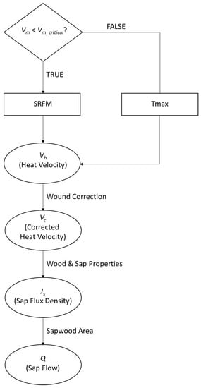
Figure 1.
The Dual Method Approach (DMA) algorithm to decide which heat velocity measurement (Vm) should be taken from HRM (heat ratio method)/SRFM (“slow rates of flow” method) of Tmax methods. The Vm_critical is a theoretically (a priori) or statistically (posteriori) determined value.
Determining SRFMmax and Tmaxmin is difficult, as it can vary with k and, possibly, other factors. A Vm_critical value can be statistically determined via a regression of Vh, as determined by the SRFM, against an independent measure of sap flow, such as a gravimetric weighing lysimeter. When correlated against an independent measure of sap flow, Vh via the SRFM will approach a plateau. A piecewise linear regression analysis, with Vh via the SRFM on the Y-axis and an independent measure of sap flow on the X-axis, can statistically determine a Vm_critical value via the breakpoint. Values below the breakpoint are assigned to the SRFM and values greater than the breakpoint are assigned to the Tmax. However, this statistical approach is practical if a sap flow sensor can be calibrated, which may not be possible for large trees. Additionally, this approach is only applicable once data has been collected and a Vm_critical value cannot be assigned prior to the commencement of a data campaign. Therefore, this statistical approach is called a posteriori analysis—an analysis derived from observational data.
An a priori analysis, or an analysis derived from theoretical deduction, can also be conducted to determine Vm_critical. The theoretical minimum and maximum Vh for Tmax and SRFM can be determined via Equations (1), (3), and (4). Tmax is typically limited by a 1 s cycle speed of contemporary data-loggers, and the SRFM is limited by the maximum value of ΔTd/ΔTu of 20 [4,7]. Furthermore, the minimum and maximum Vh for Tmax and SRFM, respectively, vary with k. The observable range in plants for k is approximately 0.0015 to 0.004 cm2/s [4,20]. Table 1 displays the minimum and maximum Vh for Tmax and SRFM, respectively, for varying k with a probe spacing of 0.6 cm and heat pulse of 3 s duration. The values in Table 1 will vary with different probe spacings and heat pulse durations.
An a priori analysis may choose with SRFMmax or Tmaxmin as the Vm_critical. However, the values listed in Table 1 are theoretical and, in practice, observable SRFMmax or Tmaxmin may be unknown. Therefore, it is proposed that the mid-point between SRFMmax and Tmaxmin is adopted for Vm_critical via the following equation:
As an example, calculation based on data presented in Table 1, for a x of 0.6 cm, a t0 of 3 s, and k of 0.0025 cm2/s, yields a Vm_critical value of 26.3 cm/h.
1.6. Converting Heat Velocity to Sap Flux Density
Once Vh has been determined via the SRFM or Tmax method for the DMA, it is necessary to correct for wounding, then convert corrected heat velocity (Vc) to sap flux density (Js).
The wound effect from insertion of probes into sapwood is corrected via Vc (cm/h):
where a, b, and c are coefficients that are calculated via finite-difference numerical modelling and vary with wound width, probe size, and spacing [7,26].
The Vc is then converted to Js (cm3/cm2/h), which is an equation that incorporates wood and sap parameters of the measured plant [27]:
2. Methods
2.1. Study Species and Plant Material
Plant material was sourced from Tecoma capensis (Thunb.) Lindl., a fast-growing southern Africa species which is an exotic weed in Australia [28]. Stems were harvested from a shrub growth form of Tecoma, 2.3 m height, in the Kingston Heath Reserve, an urban bushland in southeast Melbourne, Victoria, Australia. Ten stems were used in this study, between 1.1 and 1.3 cm in diameter and 20 cm in length, cut from eight branches from a single Tecoma shrub. Samples were harvested across two days, with four branches harvested on each day. Five stems were measured on the first day, and an additional five stems were measured on the second day. Following harvesting from the shrub, the cut end of the branch was wrapped in a moistened tissue and bagged. Samples were then taken to a nearby Implexx Sense laboratory (approx. 5 min drive) for immediate testing. In the laboratory, stems were recut underwater just prior to commencement of measurements to minimize xylem embolism.
2.2. Heat Pulse Velocity Sensor & Data Logger
A commercially available heat pulse velocity sensor (HPV-06, Implexx Sense, Melbourne, Australia) was used for measurements. The HPV-06 sensor consisted of three probes, 30 mm in length, 1.3 mm in diameter, and 6 mm axial distance apart (Figure 2). The downstream and upstream probes were temperature probes, and the central probe was the line heater. The heater probe produced 4 W to 4.9 W of power, depending on battery voltages typical of a charge cycle. Temperature measurements were made via two 10 kΩ negative temperature co-efficient (NTC) thermistors in each probe spaced at 10 mm and 20 mm consecutively from the tip of the probe. Each thermistor was wired as a Half bridge in series with a precision 24.9 kΩ resistor mounted on the circuit board in the sensor body. The accuracy of the thermistors was ±0.2 °C, and the resolution was 0.001 °C. The HPV-06 was connected to the CR1000X data-logger (Campbell Scientific, Logan, UT, USA) and individual heat-pulse events were at 10 min intervals.
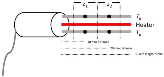
Figure 2.
An overview of the Heat Pulse Velocity Sensor’s (HPV-06) design. The positions z1 and z2 indicate the outer and inner measurement zone, respectively, with an effective measurement radial radius of 5 mm. Td and Tu represent the downstream and upstream temperature probes, respectively. Each black enclosed circle represents a thermistor measurement point. The central probe is the heater. The distance between Td or Tu and the Heater was 6 mm.
2.3. Sensor Installation
The HPV-06 sensor was installed using a drill guide into the Tecoma stem. Sections of stem internode between 1.1 and 1.3 cm diameter were chosen as sites of installation. Prior to insertion, the HPV-06 probes were lubricated with electrical grease (Inox MX6 Grease) to improve probe thermal contact with sapwood. The outer thermistor of the HPV-06 sensor was carefully positioned in the middle of the stem, as the xylem radius was ~0.5 cm and the zone of detection of the thermistor also had a ~0.5 cm radius. Therefore, positioning the thermistor in the middle of the stem captured the entire area of sapwood. Following insertion of the HPV-06 sensor in the Tecoma stem, a segment of the stem 20 cm in length, without leaves or branches, was cut underwater. This segment, with the sensor installed, remained underwater until the experimental apparatus was ready, and was immediately transferred at the commencement of measurements.
2.4. Wood Properties and Thermal Diffusivity
An additional five stem segments, ~3.0 cm in length and ~1.0 cm in diameter, were cut underwater from the sample branches for measurement of wood properties, including sapwood fresh weight, sapwood dry weight (oven-dried at 60 °C for 72 h), and sapwood fresh volume, and the subsequent calculation of mc, ρd, kHogg, and kVand, using Equations (5)–(9) (see above). The average of the five stem segments was subsequently used in converting heat velocity to sap flow and data analyses.
2.5. Heat Velocity and Sap Flux Density Measurements
During the experiment, tm and ΔTd/ΔTu were logged and later used for the calculation of Vh. Six methods to calculate Vh were used in this study: Vh_Mar with kHogg (Equations (4) and (7)), Vh_Mar with kVand (Equations (4) and (8)), Vh_Coh with kHogg (Equations (2) and (7)), Vh_Coh with kVand (Equations (2) and (8)), Vh_Klu with kHogg (Equations (3) and (7)), and Vh_Klu with kVand (Equations (3) and (8)). For each method, Vh was then converted to Vc, where the wound diameter was determined visually with a digital caliper, following Equation (11) and Burgess et al. [7]. Then, for each method, Vc was converted to Js following Equation (12).
2.6. Gravimetric Testing of Sap Flow Measurements
The accuracy of sap flux density, derived from the DMA, HRM/SRFM, and Tmax methods, was tested via a water pressure system maintaining a constant head, based on the experiments of Steppe et al. [29] and López-Bernal et al. [30]. Teflon tubing with an inner diameter of 1.3 cm was attached to the upstream end of the stem segment, and was made water- and gas-tight via pipe clamps and polytetrafluoroethylene (PTFE) thread seal tape (Kinetic Supply Pty Ltd., Broadmeadow, Australia) and was thoroughly tested for leaks. Various length tubing was connected to a water reservoir that was changed in height to create variable pressure gradients. The heights were (cm): 15, 30, 45, 60, 75, 90, 105, 120, 135, 150, 170, 200, 235, 255, and 315. At each height, flow was left to settle for at least 20 min prior to duplicate measurements at 10 min intervals. Sap passing through the downstream cut segment was collected and measured every 10 min using a three-point precision balance (WTC 200, Radwag, Radom, Poland). Concurrent sap flow data, estimated via the sap flow method and measured from the electronic balance (gravimetric sap flow), were then compared.
2.7. Statistical Analysis
Data measured on the ten stems were collated into a linear regression analysis that compared Js estimated from the Vh method against Js measured gravimetrically. Linear regression slopes were fitted through the intercept. A slope of 1, from the linear regression curve, indicated zero error between estimated and measured Js, and the R2 was a measure of precision. For the posteriori determination of Vm_critical, a piecewise linear regression model, with gravimetric Js on the X-axis and estimated Js from the sensor on the Y-axis, was used to determine the breakpoint.
3. Results
3.1. Measurement Range Limitation of SRFM and Tmax
The results confirmed the measurement range limitation of the HRM/SRFM and Tmax methods (Table 2 and Supplementary Materials). The minimum observed Vh value in this study for HRM/SRFM and Tmax, respectively, was 0.020 and 2.049 cm/h. The maximum observed Vh value for HRM/SRFM and Tmax, respectively, was 45.063 and 168.578 cm/h (Supplementary Materials).
Table 2.
Piecewise linear regression results of sap flux density (Js) estimated from the sap flow sensor method against gravimetric Js and the maximum observed (Max. Obs.) and minimum observed (Min. Obs.) heat velocity (Vh) measured for each method. A complete table comparing all methods against gravimetric sap flow is found in the Supplementary Materials. Slope was determined from the linear regression curve, and Error is based on the deviation of this slope from 1; RMSE is the root mean square error of the linear regression (smaller values indicate a more accurate model); n is sample size; Vh is heat velocity.
Sap flux density values ranged from approximately 0 to 170 cm3/cm2/h (Figure 3). However, the piecewise linear regression analysis determined that there was a breakpoint in the HRM/SRFM data at 32.540 cm3/cm2/h (Figure 4), which was considered the maximum reliable sap flux density measurement derived from the HRM/SRFM.
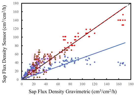
Figure 3.
Correlation between gravimetrically determined sap flux density (Js) and Js measured via HRM/SRFM (blue) and Tmax (red). The slope and R2 results are displayed in Table 2. The dashed black line is the 1:1 relationship.
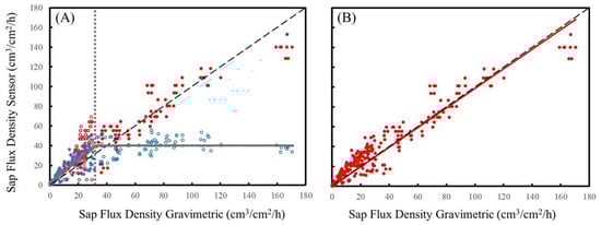
Figure 4.
An example of posteriori analysis for the DMA. (A) The piecewise linear regression analysis (solid grey line) with a breakpoint (dotted grey line) at 32.540 cm3/cm2/h. Where X <breakpoint then HRM/SRFM data is selected for the DMA, and where X >breakpoint then Tmax data is selected for the DMA, as displayed in (B). The solid red line in (B) is the linear regression of the DMA against gravimetric sap flux density. The black dashed line is the 1:1 relationship. Slopes and R2 results are displayed in Table 2.
3.2. Accuracy of HRM/SRFM, Tmax and DMA
Across the full range of measured flow, the HRM/SRFM had the lowest levels of accuracy and precision, followed by the Tmax and DMA methods (Table 2 and Supplementary Materials). The HRM/SRFM had an error between 49.1% and 63.4%, and underestimated gravimetric Js measurements. The Tmax had an error between 0.5% and 35.5% but overestimated gravimetric Js measurements. The DMA had an error between 1.2% and 29.0% and either closely estimated, or overestimated, Js measurements. The linear regression statistical analyses showed an R2 of 0.458 for HRM/SRFM, 0.807 for the Tmax and 0.888 to 0.918 for the DMA (Table 2). The results from the root mean square error (RMSE) of the linear regression analyses was consistent with this result, showing the DMA posteriori analysis as having the lowest RMSE, indicating this was the most accurate model.
An additional problem was observed with the Tmax measurements at low range. There were data points outside of the minimum measurement range (Table 1) causing errors in the calculation of Tmax at slow flows. Therefore, there was a lower sample size (n) for Tmax measurements shown in Table 2 and the Supplementary Materials.
3.3. Determination of Vm_critical and the DMA
The Vm_critical level, determined via the a priori and the posteriori methods (Figure 4) yielded similar results (Table 2). The slope of the linear regression curve of Js measured via the DMA against the gravimetric technique showed a value of 0.984 and 0.988 for the a priori and posteriori methods, respectively. The precision of the data was also similar, with an R2 of 0.888 and 0.918 for the a priori and posteriori methods, respectively. The RMSE analysis was also similar, but indicated that the posteriori approach was more accurate than the a priori approach (Table 2).
3.4. Accuracy of Cohen’s versus Kluitenberg’s Tmax Calculation
The different methods for calculating Tmax (Vh_Coh and Vh_Klu; Equations (2) and (3)) showed varying levels of accuracy and precision. The Vh_Coh equation showed better accuracy but slightly lower precision, with a linear regression curve slope of 1.005, R2 of 0.807, and RMSE of 12.816 (Supplementary Materials). The Vh_Klu equation, in contrast, resulted in a linear regression curve slope of 1.178, R2 of 0.885, and RMSE of 14.300 (Supplementary Materials). Tmax, calculated via Vh_Coh, had a smaller RMSE, indicating this model was more accurate than the Vh_Klu model.
3.5. Accuracy of Hogg’s versus Vandegehuchte’s Thermal Diffusivity (k) Calculations
The k value differed according to calculations via Hogg’s (kHogg) or Vandegehuchte’s (kVand) method. The mean kHogg value was 0.001648 cm2/s (±SD 9 × 10⁻⁵) and the mean kVand value was 0.002293 cm2/s (±SD 5 × 10⁻⁵). The difference in k resulted in different levels of accuracy when sap flux density was calculated using kHogg or kVand (Supplementary Materials). Generally, Js calculated with kHogg yielded lower accuracy and precision than Js calculated with kVand.
4. Discussion
The DMA successfully resolved the measurement range limitation of the Tmax and HRM/SRFM heat pulse velocity methods. In this study, the DMA measured near zero to extremely fast rates of sap flow. Although reverse flows were not explicitly tested in this study, the probe design and theoretical calculations suggest the DMA can also resolve upstream movement of xylem sap.
The measurement range limitation of nearly all sap flow methods has restricted their utility for research and applied applications. For example, Forster [31] demonstrated that, on average, 12% of sap flow occurs during the night, or during periods of slow sap flow, which cannot be quantified by many sap flow methods. Conversely, economically important crops, such as grapevines, are known to have fast daytime flows, which cannot be quantified by the HRM [8,10]. The DMA is a practical method to implement that can successfully quantify sap flow under these previously limiting applications.
This study advances previous attempts to combine heat pulse velocity methods to overcome the measurement range limitation. For example, Cohen et al. [32,33] combined the Tmax method and compensation heat pulse method (CHPM) for measuring slow to very high rates of flow, and Pearsall et al. [10] combined the CHPM and HRM to measure reverse, zero, slow, and high rates of flow in grapevines. The CHPM cannot measure zero or reverse flows, with one study reporting an observed minimum flow of 1.8 cm/h [34]. Therefore, the combination of CHPM with Tmax does not resolve the entire measurement range limitation observed in plants. The combination of CHPM and HRM/SRFM by Pearsall et al. [10] did overcome the measurement range limitation, as CHPM can measure high flows and HRM/SRFMcan measure slow, zero, and reverse flows. However, combining CHPM with HRM/SRFM requires either two installation sites or up to four probes [10], which can lead to errors caused by probe misalignment and wounding. The DMA advocated in this study reduces the number of probes to three, which minimizes errors caused by probe misalignment and wounding. Additionally, Pearsall et al. [10] relied on a visual assessment to determine when to switch from HRM/SRFM to CHPM, whereas a statistical and theoretical approach was demonstrated in this study to determine the Vm_critical to switch from one heat pulse velocity method to another.
4.1. Accuracy of the DMA, HRM/SRFM and Tmax
When compared with a gravimetric measure of Js, the DMA had a slope close to 1, or an error of 1.2% and an R2 >0.842. This compares with an average error of 16.9% and R2 of 0.916 for the HRM/SRFM, and an error of 35.560% and R2 of 0.859 for the Tmax reported in a meta-analysis [8]. Therefore, the DMA significantly improved the accuracy of Js estimations with similar precision to existing sap flow methods.
In this study, the HRM/SRFM poorly estimated Js, with an error between 49% and 63% (Table 2, Supplementary Materials), compared with an average error of 16.9% from a meta-analysis of 11 studies [8]. However, Vandegehuchte and Steppe [17] and Wang et al. [35] found an error of 39% and 43%, respectively, when the HRM was compared against a gravimetric measure of sap flow. Other studies testing the accuracy of the HRM found better accuracy at slow flows (e.g., [36,37]) than fast flows (e.g., [10,35]). Therefore, within its limited measurement range, the HRM may be an accurate method to estimate sap flow, but it should not be deployed on stems with fast sap fluxes.
In contrast, this study found an error as low as 0.5% for the Tmax, similar to a 0% error reported by Green [38], but contrasted with errors between 19% and 65% reported by Intrigliolo et al. [39]. The high levels of error reported by Intrigliolo et al. [39] were measured on Vitis vinifera stems, a reportedly difficult plant to measure accurately with sap flow sensors [10], and compared against a canopy gas exchange instrument. It is possible that the canopy gas exchange instrument did not accurately reflect sap flow dynamics, as it measures different plant physiological processes. The 0% error reported by Green [38] was a study also conducted on Vitis vinifera, but against a gravimetric measure of sap flow.
Heat pulse velocity sap flow sensors have an additional limitation of only measuring a small area of the potential total sapwood area in plants. In this study, this potential source of error was removed because a small stem was measured that had the same area which could be detected with the HPV-06 sap flow sensor. In other conditions, such as when measuring large trees in a forest or orchard, a heat pulse velocity sap flow sensor will potentially sample only a portion of the total cross-sectional sapwood area. Previous studies, for example Eliades et al. [40], deployed sensors at multiple sapwood radial depths and azimuthal locations to increase the sampled sapwood area of the measured tree. The DMA can overcome potential sampling errors by also measuring at multiple radial and azimuthal locations. The DMA can better address sampling issues than other heat pulse velocity methods, as it is the only method capable of measuring the entire observable range of sap flow in plants of all sizes.
4.2. Determination of Vm_critical
A statistical (posteriori) and theoretical (a priori) approach were used to determine Vm_critical, with almost identical results. The piecewise linear regression used to determine a breakpoint is a robust method to determine when the HRM/SRFM reaches its maximum measurement range. It is recommended to adopt a statistical approach, where possible, to determine Vm_critical to avoid bias and error in the estimation of the maximum HRM/SRFM measurement range. Currently, the maximum range of HRM/SRFM cannot be predicted, because the causes are varying and poorly understood [8]. It is hypothesized that at high flows, the ΔTu parameter in Equation (4) is constant whereas ΔTd decreases, leading to errors in calculating Vh [3,17]. However, it is not certain how or when this occurs. Forster [8] noted that, under extremely high flow conditions, the heat pulse travels outside the zone of measurement of the downstream temperature probe, which is possibly related to a decrease in the q parameter, or heat input, of Equation (1). The maximum range of the HRM/SRFM is also related to the plant species and its hydraulic properties. These hypotheses have not been systematically tested; therefore, it cannot currently be predicted when the HRM/SRFM will reach its maximum limit.
In many applications, it will not be feasible to wait until the end of a study period to determine Vm_critical. In such applications, the user requires reliable sap flow data in, or near, real time. The a priori method to determine Vm_critical can be adopted for such applications which, in this study, yielded almost identical results to the statistical, posteriori approach. The a priori approach used a maximum ΔTd/ΔTu ratio of 20, which was hypothesized by Marshall [4], and later used by Burgess et al. [7], to determine the maximum measurement limit of the HRM/SRFM. The importance of the ΔTd/ΔTu ratio of 20 is unknown, as Marshall nor Burgess et al. did not provide an explanation for why the value of 20 is important. In the author’s experience, ΔTd/ΔTu ratios rarely exceed 5 (personal observation); therefore, a value of 20 may be an overestimation. Values less than 20 may be equally valid in the determination of Vm_critical. A more robust examination of the optimal ΔTd/ΔTu ratio for the calculation of Vm_critical, which was outside the scope of this study, is required.
4.3. Methods to Estimate Thermal diffusivity
The k parameter in HPV calculations is critical, yet some studies adopt Marshall’s suggestion of 0.0025 cm2/s as a default value (e.g., [41]). Many studies measure k at the start or end of a measurement campaign through a stem core and the use of Equation (7) (kHogg; e.g., [42,43]). Looker et al. [20] and Vandegehuchte and Steppe [19] suggested that kHogg may underestimate k, and instead recommended the use of Equation (8) (kVand), as this method explicitly accounts for the bound and unbound moisture content of sapwood. The results of this study support the conclusion that kHogg is smaller than kVand. Furthermore, in this study Js calculated via kVand was more accurate and precise than Js calculated with kHogg. Therefore, the use of kVand may also improve the overall accuracy of sap flow measurements in general. For example, Forster [8] found that sap flow estimates from HPV methods underestimated true sap flow by an average of 34.706%. Most of the studies collated as part of Forster’s [8] meta-analysis used kHogg in calculating sap flow estimates. The use of kVand, instead, may result in improved accuracy of some of these studies, as suggested by the results of this and other studies (e.g., [44]).
5. Conclusions
The DMA successfully resolved the measurement range limitation of heat pulse velocity methods and reduced errors from as high as 63.4% to 1.2% without loss of precision. It is recommended that the DMA is adopted for sap flow measurements, rather than the HRM/SRFM or Tmax, as it supersedes the utility of these latter methods. The appropriate calculation of thermal diffusivity via using the kVand method also improved the accuracy of sap flow measurements.
Supplementary Materials
The following are available online at http://www.mdpi.com/1999-4907/10/1/46/s1, Supplementary Material S1: Detailed results from the piecewise linear regression analysis of the various sap flow methods against gravimetric measurements of sap flow.
Conflicts of Interest
The author is an owner of Implexx Sense—a company that manufactures and distributes sap flow sensors commercially.
References
- Kim, H.K.; Park, J.; Hwang, I. Investigating water transport through the xylem network in vascular plants. J. Exp. Bot. 2014, 65, 1895–1904. [Google Scholar] [CrossRef] [PubMed]
- Steppe, K.; Vandegehuchte, M.W.; Tognetti, R.; Mencuccini, M. Sap flow as a key trait in the understanding of plant hydraulic functioning. Tree Physiol. 2015, 35, 341–345. [Google Scholar] [CrossRef] [PubMed]
- Vandegehuchte, M.W.; Steppe, K. Sap-flux density measurement methods: Working principles and applicability. Funct. Plant Biol. 2013, 40, 213–223. [Google Scholar] [CrossRef]
- Marshall, D.C. Measurement of sap flow in conifers by heat transport. Plant Physiol. 1958, 33, 385–396. [Google Scholar] [CrossRef] [PubMed]
- Cohen, Y.; Fuchs, M.; Green, G.C. Improvement of the heat pulse method for determining sap flow in trees. Plant Cell Environ. 1981, 4, 391–397. [Google Scholar] [CrossRef]
- Green, S.R.; Clothier, B.; Jardine, B. Theory and practical application of heat pulse to measure sap flow. Agron. J. 2003, 95, 1371–1379. [Google Scholar] [CrossRef]
- Burgess, S.S.O.; Adams, M.A.; Turner, N.C.; Beverly, C.R.; Ong, C.K.; Khan, A.A.H.; Bleby, T.M. An improved heat-pulse method to measure low and reverse rates of sap flow in woody plants. Tree Physiol. 2001, 21, 589–598. [Google Scholar] [CrossRef]
- Forster, M.A. How reliable are heat pulse velocity methods for estimating tree transpiration? Forests 2017, 8, 350. [Google Scholar] [CrossRef]
- Bleby, T.M.; McElrone, A.J.; Burgess, S.S.O. Limitations of the HRM: Great at low flow rates, but no yet up to speed? In Proceedings of the 7th International Workshop on Sap Flow: Book of Abstracts, Seville, Spain, 22–24 October 2008.
- Pearsall, K.R.; Williams, L.E.; Castorani, S.; Bleby, T.M.; McElrone, A.J. Evaluating the potential of a novel dual heat-pulse sensor to measure volumetric water use in grapevines under a range of flow conditions. Funct. Plant Biol. 2014, 41, 874–883. [Google Scholar] [CrossRef]
- Clearwater, M.J.; Luo, Z.; Mazzeo, M.; Dichio, B. An external heat pulse method for measurement of sap flow through fruit pedicels, leaf petioles and other small-diameter stems. Plant Cell Environ. 2009, 32, 1652–1663. [Google Scholar] [CrossRef]
- Green, S.R.; Romero, R. Can we improve heat-pulse to measure low and reverse flows? Acta Hortic. 2012, 951, 19–29. [Google Scholar] [CrossRef]
- Green, S.; Clothier, B.; Perie, E. A re-analysis of heat pulse theory across a wide range of sap flows. Acta Hortic. 2009, 846, 95–104. [Google Scholar] [CrossRef]
- Ferreira, M.I.; Green, S.; Conceição, N.; Fernández, J. Assessing hydraulic redistribution with the compensated average gradient heat-pulse method on rain-fed olive trees. Plant Soil 2018, 425, 21–41. [Google Scholar] [CrossRef]
- Romero, R.; Muriel, J.L.; Garcia, I.; Green, S.R.; Clothier, B.E. Improving heat-pulse methods to extend the measurement range including reverse flows. Acta Hortic. 2012, 951, 31–38. [Google Scholar] [CrossRef]
- Testi, L.; Villalobos, F. New approach for measuring low sap velocities in trees. Agric. Meteorol. 2009, 149, 730–734. [Google Scholar] [CrossRef]
- Vandegehuchte, M.W.; Steppe, K. Sapflow+: A four-needle heat-pulse sap flow sensor enabling nonempirical sap flux density and water content measurements. New Phytol. 2012, 196, 306–317. [Google Scholar] [CrossRef] [PubMed]
- Kluitenberg, G.J.; Ham, J.M. Improved theory for calculating sap flow with the heat pulse method. Agric. For. Meteorol. 2004, 126, 169–173. [Google Scholar] [CrossRef]
- Vandegehuchte, M.W.; Steppe, K. Improving sap-flux density measurements by correctly determining thermal diffusivity, differentiating between bound and unbound water. Tree Physiol. 2012, 32, 930–942. [Google Scholar] [CrossRef]
- Looker, N.; Martin, J.; Jencso, K.; Hu, J. Contribution of sapwood traits to uncertainty in conifer sap flow as estimated with the heat-ratio method. Agric. For. Meteorol. 2016, 223, 60–71. [Google Scholar] [CrossRef]
- Edwards, W.R.N.; Warwick, N.W.M. Transpiration from a kiwifruit vine as estimated by the heat pulse technique and the Penman-Monteith equation. N. Z. J. Agric. Res. 1984, 27, 537–543. [Google Scholar] [CrossRef]
- Becker, P.; Edwards, W.R.N. Corrected heat capacity of wood for sap flow calculations. Tree Physiol 1999, 19, 767–768. [Google Scholar] [CrossRef]
- Hogg, E.H.; Black, T.A.; den Hartog, G.; Neumann, H.H.; Zimmermann, R.; Hurdle, P.A.; Blanken, P.D.; Nesic, Z.; Yang, P.C.; Staebler, R.M.; et al. A comparison of sap flow and eddy fluxes of water vapor from a boreal deciduous forest. J. Geophys. Res. 1997, 102, 28929–28937. [Google Scholar] [CrossRef]
- Barkas, W.W. Fibre saturation point of wood. Nature 1935, 135, 545. [Google Scholar] [CrossRef]
- Kollmann, F.F.P.; Cote, W.A., Jr. Principles of Wood Science and Technology: Solid Wood; Springer: Berlin Heidelberg, Germany, 1968. [Google Scholar]
- Swanson, R.H.; Whitfield, D.W.A. A numerical analysis of heat pulse velocity and theory. J. Exp. Bot. 1981, 32, 221–239. [Google Scholar] [CrossRef]
- Barrett, D.J.; Hatton, T.J.; Ash, J.E.; Ball, M.C. Evaluation of the heat pulse velocity technique for measurement of sap flow in rainforest and eucalypt forest species of south-eastern Australia. Plant Cell Environ. 1995, 18, 463–469. [Google Scholar] [CrossRef]
- Biosecurity Queensland. Environmental Weeds of Australia for Biosecurity Queensland Edition; Queensland Government: Brisbane, Australia, 2016.
- Steppe, K.; de Pauw, D.J.W.; Doody, T.M.; Teskey, R.O. A comparison of sap flux density using thermal dissipation, heat pulse velocity and heat field deformation methods. Agric. For. Meteorol. 2010, 150, 1046–1056. [Google Scholar] [CrossRef]
- López-Bernal, A.; Testi, L.; Villalobos, F.J. A single-probe heat pulse method for estimating sap velocity in trees. New Phytol. 2017, 216, 321–329. [Google Scholar] [CrossRef] [PubMed]
- Forster, M.A. How significant is nocturnal sap flow? Tree Physiol. 2014, 34, 757–765. [Google Scholar] [CrossRef] [PubMed]
- Cohen, Y.; Fuchs, M.; Falkenflug, V.; Moreshet, S. Calibrated heat pulse method for determining water uptake in cotton. Agron. J. 1988, 80, 398–402. [Google Scholar] [CrossRef]
- Cohen, Y.; Takeuchi, S.; Nozaka, J.; Yano, T. Accuracy of sap flow measurement using heat balance and heat pulse methods. Agron. J. 1993, 85, 1080–1086. [Google Scholar] [CrossRef]
- Lassoie, J.P.; Scott, D.R.M.; Fritschen, L.J. Transpiration studies in Douglas-fir using the heat pulse technique. For. Sci. 1977, 23, 377–390. [Google Scholar]
- Wang, S.; Fan, J.; Wang, Q. Determining evapotranspiration of a Chinese Willow stand with three-needle heat-pulse probes. Soil Sci. Soc. Am. J. 2015, 79, 1545–1555. [Google Scholar] [CrossRef]
- Bleby, T.M.; Burgess, S.S.O.; Adams, M.A. A validation, comparison and error analysis of two heat-pulse methods for measuring sap flow in Eucalyptus marginata saplings. Funct. Plant Biol. 2004, 31, 645–658. [Google Scholar] [CrossRef]
- Madurapperuma, W.S.; Bleby, T.M.; Burgess, S.S.O. Evaluation of sap flow methods to determine water use by cultivated palms. Environ. Exp. Bot. 2009, 66, 372–380. [Google Scholar] [CrossRef]
- Green, S.R. Measurement and modelling the transpiration of fruit trees and grapevines for irrigation scheduling. Acta Hortic. 2008, 792, 321–332. [Google Scholar] [CrossRef]
- Intrigliolo, D.S.; Lakso, A.N.; Piccioni, R.M. Grapevine cv. ‘Riesling’ water use in the northeastern United States. Irrig. Sci. 2009, 27, 253–262. [Google Scholar] [CrossRef]
- Eliades, M.; Bruggeman, A.; Djuma, H.; Lubczynski, M. Tree water dynamics in a semi-arid, Pinus brutia forest. Water 2018, 10, 1039. [Google Scholar] [CrossRef]
- Zhao, C.Y.; Si, J.H.; Qi, F.; Yu, T.F.; Li, P.D. Comparative study of daytime and nighttime sap flow of Populus euphratica. Plant Growth Regul. 2017, 82, 353–362. [Google Scholar] [CrossRef]
- Deng, Z.; Guan, H.; Hutson, J.; Forster, M.A.; Wang, Y.; Simmons, C.T. A vegetation focused soil-plant-atmospheric continuum model to study hydrodynamic soil-plant water relations. Water Resour. Res. 2017, 53, 4965–4983. [Google Scholar] [CrossRef]
- Doronila, A.I.; Forster, M.A. Performance measurement via sap flow monitoring of three Eucalyptus species for mine site and dryland salinity phytoremediation. Int. J. Phytoremed. 2015, 17, 101–108. [Google Scholar] [CrossRef]
- López-Bernal, Á.; Alcántara, E.; Villalobos, F.J. Thermal properties of sapwood fruit trees as affected by anatomy and water potential: Errors in sap flux density measurements based on heat pulse methods. Trees 2014, 28, 1623–1634. [Google Scholar] [CrossRef]


© 2019 by the author. Licensee MDPI, Basel, Switzerland. This article is an open access article distributed under the terms and conditions of the Creative Commons Attribution (CC BY) license (http://creativecommons.org/licenses/by/4.0/).