Article

Noncircular Sources-Based Sparse Representation Algorithm for Direction of Arrival Estimation in MIMO Radar with Mutual Coupling

College of Automation, Harbin Engineering University, Harbin 150001, China
*
Author to whom correspondence should be addressed.
Algorithms 2016, 9(3), 61; https://doi.org/10.3390/a9030061
Submission received: 25 June 2016 / Revised: 1 September 2016 / Accepted: 2 September 2016 / Published: 8 September 2016

Abstract

:
In this paper, a reweighted sparse representation algorithm based on noncircular sources is proposed, and the problem of the direction of arrival (DOA) estimation for multiple-input multiple-output (MIMO) radar with mutual coupling is addressed. Making full use of the special structure of banded symmetric Toeplitz mutual coupling matrices (MCM), the proposed algorithm firstly eliminates the effect of mutual coupling by linear transformation. Then, a reduced dimensional transformation is exploited to reduce the computational complexity of the proposed algorithm. Furthermore, by utilizing the noncircular feature of signals, the new extended received data matrix is formulated to enlarge the array aperture. Finally, based on the new received data, a reweighted matrix is constructed, and the proposed method further designs the joint reweighted sparse representation scheme to achieve the DOA estimation by solving the l 1 -norm constraint minimization problem. The proposed method enlarges the array aperture due to the application of signal noncircularity, and in the presence of mutual coupling, the proposed algorithm provides higher resolution and better angle estimation performance than ESPRIT-like, l 1 -SVD and l 1 -SRDML (sparse representation deterministic maximum likelihood) algorithms. Numerical experiment results verify the effectiveness and advantages of the proposed method.

1. Introduction

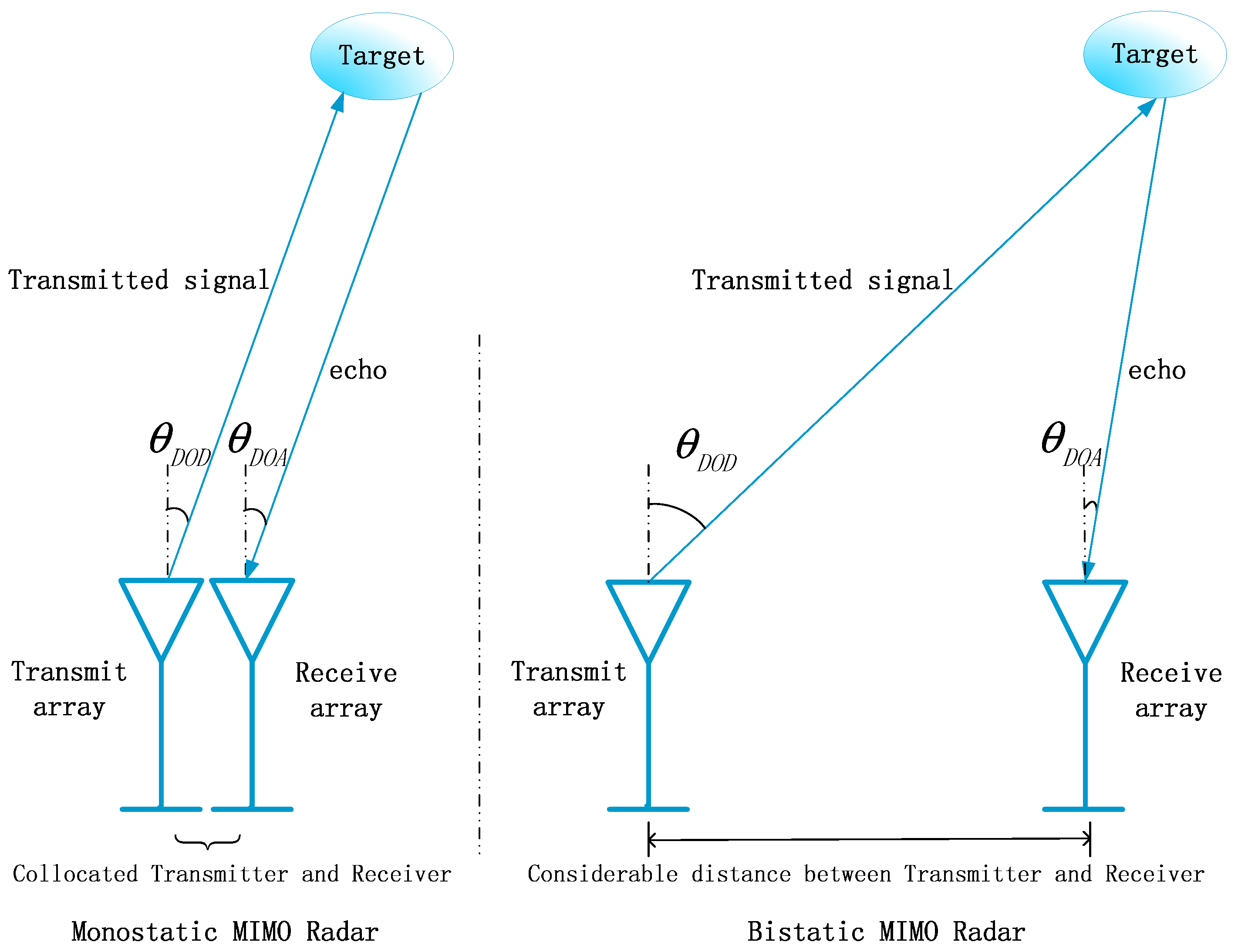
With orthogonal transmitted waveforms, multiple-input multiple-output (MIMO) radar has drawn increasing attention in the field of wireless communications. Compared with the conventional phased-array radar, MIMO radar owns a number of advantages, such as higher resolution and better parameter identifiability [1]. In addition, MIMO radar can be classified into the following two types: statistical MIMO radar and colocated MIMO radar. Colocated MIMO radar can achieve more degrees of freedom and higher spatial resolution, because its closely-spaced antennas form a virtual array with a large aperture. Colocated MIMO radar includes the monostatic one and the bistatic one. In bistatic MIMO radar, the transmit array and the receive array are separated away, while they are close to each other in monostatic MIMO radar. In this paper, the angle estimation problem is investigated in monostatic MIMO radar.
Parameter estimation is an important aspect in wireless communications and sensor array signal processing [2]. In order to estimate the direction of arrival (DOA), a large number of subspace-based algorithms have been proposed [3,4,5]. Recently, the emerging sparse representation (SR) and compressed sensing (CS) have attracted more and more attention in various fields [6,7,8], such as sensor array signal processing, imaging and image processing, and so forth. Furthermore, it has been verified that SR-based DOA estimation algorithms have remarkable advantages over other methods [9], for instance they adapt better to challenging circumstances and provide higher angle resolution. A few SR-based algorithms, such as l 1 -SVD (singular value decomposition) [9] and l 1 -SRACV (array covariance vectors) [10], have been proposed via sparse signal recovery. In [11], based on the array covariance vector, the revised real-valued (RV) l 1 -SVD approach has better DOA estimation performance and lower computation burden than l 1 -SVD [9] and RV l 1 -SVD [12].
However, in practical situations, the sensor array manifold is often affected by the errors of unknown mutual coupling. When they are taken into account, the DOA estimation performance of the above-mentioned methods is seriously degraded. With mutual coupling, the subspace-based MUSIC-like (multiple signal classification-like) [13] algorithm is proposed. Besides, a ESPRIT-like (estimation of signal parameters via rotational invariance techniques-like) algorithm is presented in [14], which owns a low calculation burden. In [15], the SR-based revised l 1 -SVD algorithm eliminates the errors of mutual coupling, and it achieves angle estimation by solving the problem of the l 1 -norm constraint minimization. In [16], in the presence of mutual coupling, by introducing the refined deterministic maximum likelihood (DML) procedure, a covariance vector-based sparse representation algorithm is proposed with outstanding angle estimation performance. We call the method in [16] l 1 -SRDML (sparse representation deterministic maximum likelihood).
In practical communication systems and radar applications, the complex noncircular sources are widely used, such as binary phase shift keying (BPSK), multiple amplitude shift keying (MASK) and unbalanced quadrature phase shift keying (UQPSK) modulated signals [17]. Noncircular signals can be used to enlarge the array aperture without extra antennas, which contributes to the improvement of angle estimation performance [18]. Exploiting the signal noncircularity, some subspace-based methods have been developed for angle estimation in MIMO radar [17,19,20]. They have verified that compared with traditional subspace-based algorithms, the methods that are based on noncircular signals can achieve better DOA estimation performance. However, these subspace-based approaches do not take the errors of unknown mutual coupling into account. Moreover, they perform poorly when experiencing challenging circumstances, such as fewer snapshots, which can be solved by sparse representation-based methods. For DOA estimation in MIMO radar with mutual coupling, to the best of our knowledge, up to now, there are no references about SR-based methods that exploit the signal noncircularity to extend the virtual array. Consequently, utilizing noncircular sources and the sparse representation framework, we aim to eliminate the effect of mutual coupling and then achieve a better DOA estimation.
In this paper, by using the noncircular signals, we propose a sparse representation-based DOA estimation algorithm in MIMO radar with mutual coupling. The new method firstly eliminates the effect of mutual coupling by extracting the information of mutual coupling coefficients into a diagonal matrix. Secondly, based on the reduced dimensional transformation and the characteristics of signal noncircularity, the new extended received data matrix is formulated to enlarge the array aperture. Finally, a reweighted matrix is constructed, based on which a joint reweighted l 1 -norm minimization sparse representation framework is designed to obtain the DOAs. In the presence of mutual coupling, the proposed algorithm performs better than the conventional algorithms on account of the error elimination and the application of noncircular signals.
The rest of this paper is organized as follows. In Section 2, the MIMO radar system model with mutual coupling and noncircular signals is described. In Section 3, the implementation process of the proposed method is described in detail, including mutual coupling elimination, noncircular signal-based extended matrix construction and the joint reweighted sparse representation-based DOA estimation scheme. In Section 4, we give some related remarks and discussions regarding the parameter setting and the computational complexity of the proposed method. Then, in Section 5, simulations are implemented to verify the efficiency and the advantages of the proposed method. Finally, our conclusions are summarized in Section 6.
Notation: ( · ) H , ( · ) T , ( · ) * , ( · ) 1 , E ( · ) and det ( · ) denote conjugate-transpose, transpose, conjugate, inverse, expectation and determinant operators, respectively. ⊗ and ⊙ denote the Kronecker product and the Khatri–Rao product, respectively. I K denotes a K × K dimensional unit matrix. · 1 , · 2 and · F denote the l 1 -norm, the l 2 -norm and the Frobenius-norm, respectively. diag ( · ) denotes the diagonalization operation.

2. Problem Formulation

2.1. MIMO Radar System Model with Mutual Coupling

Consider a narrowband monostatic MIMO radar system, shown in Figure 1, whose transmit and receive arrays are both half-wavelength d spaced uniform linear arrays (ULAs). In the transmit array, M antennas transmit M orthogonal noncircular waveforms, such as BPSK modulated signals. In the receive array, N antennas are impinged by P uncorrelated targets that can be deemed as point scatterers in the far-field. Different from the mutually-separated arrays in bistatic MIMO radar, the transmitter and the receiver are closely located in monostatic radar, as shown in Figure 2. Since the transmit array and the receive array are collocated at the same site in monostatic MIMO radar systems [17], the echo signal travels the same path as the transmitted signal. Therefore, for the p-th target, the directions of departure of the transmitted signal and arrival of the echo from the target are the same [21], i.e., θ D O D = θ D O A , both of which are denoted as DOA θ p , p = 1 , 2 , P . When mutual coupling is taken into account in both the transmit array and the receive array, at the receiver, the output of the matched filters at a certain snapshot is given by [16]:
x ( t ) = A ˜ s ( t ) + n ( t )
where x ( t ) C M N × 1 is the received data vector, s ( t ) = [ s 1 ( t ) , s 2 ( t ) , , s P ( t ) ] T C P × 1 is the complex-valued noncircular signal vector and n ( t ) C M N × 1 is the additional Gaussian noise vector with zero-mean and covariance matrix σ 2 I M N , in which σ 2 is the noise power. Meanwhile, the detailed expression of A ˜ is [14]:
A ˜ = [ C t a t ( θ 1 ) C r a r ( θ 1 ) , , C t a t ( θ P ) C r a r ( θ P ) ] = ( C t C r ) [ a t ( θ 1 ) a r ( θ 1 ) , , a t ( θ P ) a r ( θ P ) ]
where A ˜ C M N × P , a t ( θ p ) = [ 1 , e j π sin ( θ p ) , e j π 2 sin ( θ p ) , , e j π ( M 1 ) sin ( θ p ) ] T is the transmit steering vector and a r ( θ p ) = [ 1 , e j π sin ( θ p ) , e j π 2 sin ( θ p ) , , e j π ( N 1 ) sin ( θ p ) ] T is the receive steering vector, p = 1 , 2 , P . C t and C r are mutual coupling matrices of the transmit array and the receive array, respectively. C t and C r can be modeled as banded symmetric Toeplitz matrices, which are expressed as [22,23,24]:
C i = c i 0 c i 1 c i k 0 c i 1 c i 0 c i 1 c i 1 c i 0 c i k c i k c i 1 c i 1 c i 0 c i 1 0 c i k c i 1 c i 0
where i = t , r , c i j is the non-zero mutual coupling coefficient, j = 0 , 1 , . . . , k . In Figure 1, the coupling effects of the m-th and the n-th elements in the transmit and the receive arrays are described, respectively. β ( m , q ) is the coupling contribution from the q-th to the m-th elements in transmit array, and β ¯ ( n , q ) is the contribution from the q -th to the n-th elements in the receive array, 1 m M , 1 n N , and | q m | k , | q n | k . β ( m , q ) and β ¯ ( n , q ) contain the information of c t | q m | and c r | q n | , respectively. Mutual coupling coefficients are factors related to the distance between the two antennas [23], and for the k + 1 non-zero coefficients, they satisfy 0 <   | c i k |   <   . . .   <   | c i 1 |   <   | c i 0 |   =   1 . Besides, for the ULA coupling model, just a few mutual coupling coefficients are non-zero ones [22,23,24], and without loss of generality, 2 k < min { M , N } is assumed. Then, by collecting J snapshots, the received data in MIMO radar with mutual coupling is represented as follows:
X = C A S + N
where X C M N × J is the data matrix, C = ( C t C r ) C M N × M N is the transmit-receive mutual coupling matrix. A = [ a ( θ 1 ) , , a ( θ P ) ] C M N × P is the steering matrix, with the steering vector a ( θ p ) = a t ( θ p ) a r ( θ p ) , p = 1 , 2 , P . S = [ s ( t 1 ) , , s ( t J ) ] C P × J and N = [ n ( t 1 ) , , n ( t J ) ] C M N × J are the noncircular signal matrix and the complex Gaussian white noise matrix, respectively.

2.2. Noncircular Signals

For complex random variables and vectors, circularity is an important property [18]. Making full use of the properties of noncircular signals, the array aperture can be enlarged. The invariance specialityof rotation can be used to judge if a complex random sequence is noncircular [18]. More specifically, if stationary complex signal sequence q ¯ is circular, it accords with E [ q ¯ q ¯ H ] 0 and E [ q ¯ q ¯ T ] = 0 . By comparison, if the sequence is noncircular, then E [ q ¯ q ¯ H ] 0 and E [ q ¯ q ¯ T ] 0 , which can be utilized to increase the number of effective array elements. In addition, for zero-mean stationary complex signal sequence q ¯ , it holds the property that:
E [ q ¯ q ¯ T ] = ρ e j ψ E [ q ¯ q ¯ H ]
where 0 ρ 1 and ψ are noncircular rate and noncircular phase angle, respectively, and ρ depends on the signal modulation type. In this paper, we consider the signals with maximum noncircular rate, namely, ρ = 1 in s ( t ) , such as BPSK and MASK modulated signals that are widely used in MIMO radar systems. It has been pointed out that the noncircular signal vector s ( t ) in Equation (1) can be rewritten as [17,25]:
s ( t ) = Λ φ s r ( t )
where s r ( t ) = [ s r 1 ( t ) , s r 2 ( t ) , , s r P ( t ) ] T is the real-valued part of noncircular signal s ( t ) , and Λ φ = diag ( [ e j φ 1 , e j φ 2 , , e j φ P ] ) is the noncircular phase matrix. Based on the composition and structure of s ( t ) , for the p-th target with t = 1 , 2 , , J , E [ s p s p T ] = e j 2 φ p E [ s r p s r p T ] = e j 2 φ p E [ s p s p H ] can be obtained. In addition, each element in s ( t ) accords with Equation (5), i.e., E [ s p s p T ] = e j ψ E [ s p s p H ] with ρ = 1 [26]. This indicates that the relationship between φ p and ψ p can be written as φ p = ψ p / 2 . With the application of signal noncircularity, X in Equation (4) is expressed as:
X = C A Λ φ S r + N
where S r = [ s r ( t 1 ) , , s r ( t J ) ] is a real-valued matrix.

3. The Proposed Algorithm

3.1. Mutual Coupling Elimination

To successfully implement the noncircular source-based sparse representation method, we firstly eliminate the effect of mutual coupling. Exploiting the structure of mutual coupling matrices C t and C r , we define two selection matrices as follows:
Γ 1 = [ 0 ( M 2 k ) × k I ( M 2 k ) × ( M 2 k ) 0 ( M 2 k ) × k ] Γ 2 = [ 0 ( N 2 k ) × k I ( N 2 k ) × ( N 2 k ) 0 ( N 2 k ) × k ]
where Γ 1 C ( M 2 k ) × M , and Γ 2 C ( N 2 k ) × N . Γ 1 and Γ 2 can be used to choose the central rows of the mutual coupling matrices and then transform the transmit-receive mutual coupling matrix C into a diagonal one. Thus, let z p = e j π sin ( θ p ) , by multiplying the selection matrix Γ 1 on the left side of the transmit steering vector with mutual coupling; the transformation of the i-th element in Γ 1 C t a t ( θ p ) C ( M 2 k ) × 1 can be derived as:
[ Γ 1 C t a t ( θ p ) ] ( i ) = c t k z p i 1 + c t ( k 1 ) z p i + + z p i + k 1 + + c t k z p i + k 1 + k = ( j = k k c t | j | z p j + k ) z p i 1 = ω t p z p i 1
where ω t p is a scalar that just contains the information of θ p and mutual coupling in the transmit array. Let M ¯ = M 2 k ; thus, for i = 1 , 2 , , M ¯ , we have Γ 1 C t a t ( θ p ) = ω t p a ˜ t , in which a ˜ t is the new transmit steering vector and can be expressed as a ˜ t = [ 1 , z p , z p 2 , z p M ¯ 1 ] , p = 1 , 2 , , P . Similar to Equation (9), we use the other selection matrix Γ 2 to extract the mutual coupling coefficients in C r a r ( θ p ) into a scalar, that is:
[ Γ 1 C r a r ( θ p ) ] ( i ) = c r k z p i 1 + c r ( k 1 ) z p i + + z p i + k 1 + + c r k z p i + k 1 + k = ( j = k k c r | j | z p j + k ) z p i 1 = ω r p z p i 1
where p = 1 , 2 , , P . The value of ω r p depends on the mutual coupling coefficients and θ p . Then, for i = 1 , 2 , , N ¯ , we further have Γ 2 C r a r ( θ p ) = ω r p a ˜ r with a ˜ r = [ 1 , z p , z p 2 , z p N ¯ 1 ] being the new receive steering vector. As a result, exploiting the property of the Kronecker product operator, let Γ = Γ 1 Γ 2 C M ¯ N ¯ × M N be the selection matrix of transmit-receive array; we deduce that:
Γ C a ( θ p ) = [ Γ 1 C t a t ( θ p ) ] [ Γ 2 C r a r ( θ p ) ] = ω t p ω r p a ˜ ( θ p )
where a ˜ ( θ p ) = a ˜ t ( θ p ) a ˜ r ( θ p ) C M ¯ N ¯ × 1 is the new transmit-receive steering vector. Thus, for J snapshots, the data matrix X in Equation (7) transfers into:
X ¯ = A ¯ D Λ φ S r + N ¯
where A ¯ = [ a ˜ ( θ 1 ) , a ˜ ( θ 2 ) , , a ˜ ( θ P ) ] C M ¯ N ¯ × P and N ¯ = Γ N C M ¯ N ¯ × J are the new transmit-receive steering matrix and noise matrix, respectively; in addition, D = diag [ ω t 1 ω r 1 , ω t 2 ω r 2 , , ω t P ω r P ] C P × P . It can be observed in Equation (12) that non-zero mutual coupling coefficients are extracted into a diagonal matrix D . Hence, for the new steering matrix A ¯ , the errors of mutual coupling are eliminated.

3.2. Noncircular Signal-Based Extended Matrix Construction

Based on the new received data matrix X ¯ , a reduced dimensional transformation is introduced in the following. For the p-th target, the transmit-receive steering vector a ˜ ( θ p ) can be expressed as:
a ˜ ( θ p ) = ( 1 , , z p N ¯ 1 ; z p , , z p N ¯ ; ; z p M ¯ 1 , , z p M ¯ + N ¯ 2 ) T
where p = 1 , 2 , , P . Many repeated terms are contained in a ˜ ( θ p ) , and the non-repeated elements can make up another vector b ( θ p ) = [ 1 , exp ( j π sin θ p ) , , exp ( j π ( M ¯ + N ¯ 2 ) sin θ p ) ] T C ( M ¯ + N ¯ 1 ) × 1 . The relationship between a ˜ ( θ p ) and b ( θ p ) can be derived as a ˜ ( θ p ) = Gb ( θ p ) , in which G is represented as:
G = [ L 0 T , L 1 T , , L M ¯ 1 T ] T
where G C M ¯ N ¯ × ( M ¯ + N ¯ 1 ) , and L m = [ 0 N ¯ × m , I N ¯ , 0 N ¯ × ( M ¯ m 1 ) ] C N ¯ × ( M ¯ + N ¯ 1 ) for m = 0 , 1 , . . . , M ¯ 1 . Thus, based on G , a reduced dimensional transformation matrix can be constructed as R = ( G H G ) ( 1 2 ) G H , then X ¯ in Equation (12) turns into:
Y = ( G H G ) ( 1 2 ) G H G B D Λ φ S r + R N ¯ = F B D Λ φ S r + N ¯ d
where Y and N ¯ d = R N ¯ are the new reduced dimensional data matrix and the new noise matrix, respectively. F = ( G H G ) ( 1 2 ) C ( M ¯ + N ¯ 1 ) × ( M ¯ + N ¯ 1 ) can be directly calculated as:
F = diag [ 1 , 2 , . . . , min ( M ¯ , N ¯ ) , . . . , min ( M ¯ , N ¯ ) | M ¯ N ¯ | + 1 , . . . . , 2 , 1 ]
By the transformation, the dimension of the data matrix is reduced from M ¯ N ¯ × J to ( M ¯ + N ¯ 1 ) × J . In addition, as R R H = I M ¯ + N ¯ 1 , the transformation does not bring in the additional spatial colored noises. In order to enlarge the array aperture by exploiting the noncircular signals, the new received data matrix Y C ( M ¯ + N ¯ 1 ) × J can be extended as Z = [ Y T , Y H ] T C 2 ( M ¯ + N ¯ 1 ) × J . Since F , D and S r are real-valued matrices, Z is expressed as:
Z = F B D Λ φ F B * D Λ φ * S r + N ¯ d N ¯ d *

3.3. Joint Reweighted Sparse Representation-Based DOA Estimation Scheme

In order to successfully apply the sparse representation theory to estimate the DOAs, we bring in the SVD technique of Z , i.e., Z = U Λ V H , where Λ = diag ( ω 1 , ω 2 , , ω M ¯ + N ¯ 1 ) , and ω 1 ω 2 ω M ¯ + N ¯ 1 are singular values. Let V s be composed of the P vectors in V that correspond to ( ω 1 , ω 2 , , ω P ) . With V s , the dimension of the observation matrix can be further reduced [9], which is conducive to the signal reconstruction, that is:
Z v = F B D Λ φ S r V s F B * D Λ φ * S r V s + N ¯ d V s N ¯ d * V s = B ¯ T ¯ B ˜ T ˜ + N ¯ d s N ˜ d s
where Z v = Z V s C 2 ( M ¯ + N ¯ 1 ) × P , B ¯ = F B , T ¯ = D Λ φ S r V s , B ˜ = F B * , T ˜ = D Λ φ * S r V s , N ¯ d s and N ˜ d s are the new noise matrices. Z v can be divided into the following two parts; the first ( M ¯ + N ¯ 1 ) rows in Z v make up Z v 1 C ( M ¯ + N ¯ 1 ) × P , and the remaining rows compose Z v 2 C ( M ¯ + N ¯ 1 ) × P , namely Z v = [ Z v 1 T , Z v 2 T ] T . By constructing two complete dictionaries B ¯ θ ^ = F [ b ( θ ^ 1 ) , b ( θ ^ 2 ) , , b ( θ ^ L ) ] and B ˜ θ ^ = F [ b * ( θ ^ 1 ) , b * ( θ ^ 2 ) , , b * ( θ ^ L ) ] with { θ ^ l } l = 1 L ( L P ) being the discretized sampling grids of all potential DOAs, the corresponding sparse representation models can be separately formulated as:
Z v 1 = B ¯ θ ^ T ¯ θ ^ + N ¯ d s Z v 2 = B ˜ θ ^ T ˜ θ ^ + N ˜ d s
where T ¯ θ ^ C L × P and T ˜ θ ^ C L × P hold the same row support with T ¯ and T ˜ , respectively. For the two models in Equation (19), if they are solved independently by conventional sparse representation methods that are based on the l 1 -norm penalty [9], the signal noncircularity cannot be utilized to extend the array aperture. In order to make the best of signal noncircularity, we design a joint sparse vector r C L × 1 whose k-th element is r ( k ) = ( T ¯ θ ^ ( l 2 ) ( k ) ) 2 + ( T ˜ θ ^ ( l 2 ) ( k ) ) 2 , then the sparsities of T ¯ θ ^ and T ˜ θ ^ are combined. In r ( k ) , T ¯ θ ^ ( l 2 ) ( k ) and T ˜ θ ^ ( l 2 ) ( k ) are defined as T ¯ θ ^ ( l 2 ) ( k ) = T ¯ θ ^ ( k , : ) 2 and T ˜ θ ^ ( l 2 ) ( k ) = T ˜ θ ^ ( k , : ) 2 , respectively. More specifically, T ¯ θ ^ ( l 2 ) ( k ) is equal to the l 2 -norm of the k-th row in T ¯ θ ^ ; similarly, T ˜ θ ^ ( l 2 ) ( k ) is equal to the l 2 -norm of the k-th row in T ˜ θ ^ . Let r ^ represent the solution vector of the sparse signal reconstruction, r ^ ( k ) r ( k ) , k = 1 , 2 , , L . As a result, based on the l 1 -norm constrained minimization, a joint sparse representation scheme is designed as follows:
min r ^ 1 , s . t .   Z v 1 B ¯ θ ^ T ¯ θ ^ F 2 η 1 Z v 2 B ˜ θ ^ T ˜ θ ^ F 2 η 2
where η 1 and η 2 are regularization parameters that set the error amount. To make the l 1 -norm penalty better approximate the l 0 -norm penalty, we introduce the reweighted matrix in the following. Let U n be the noise subspace and composed of the ( M ¯ + N ¯ 1 P ) vectors in U n that correspond to ( ω P + 1 , ω P + 2 , , ω M ¯ + N ¯ 1 ) . According to the subspace principle [13], for the true target θ p , [ ( ω t p ω r p e j φ p F b ( θ p ) ) T , ( ω t p ω r p e j φ p F b ( θ p ) * ) T ] T in Z is orthogonal to the noise subspace U n , that is:
Q ( θ p , φ p , ω t p , ω r p ) = [ ω t p ω r p e j φ p ω t p ω r p e j φ p ] Q ¯ ( θ p ) ω t p ω r p e j φ p ω t p ω r p e j φ p 0
where:
Q ¯ ( θ p ) = F b ( θ p ) 0 ( M ¯ + N ¯ 1 ) × 1 0 ( M ¯ + N ¯ 1 ) × 1 F b * ( θ p ) H U n U n H F b ( θ p ) 0 ( M ¯ + N ¯ 1 ) × 1 0 ( M ¯ + N ¯ 1 ) × 1 F b * ( θ p )
Since Q ( θ p , φ p , ω t p , ω r p ) 0 , ω t p , ω r p and e j φ p are all non-zero scalars and the rank of U n U n H satisfies rank ( U n U n H ) > 2 , for the true DOA θ p , the rank reduction of Q ¯ ( θ p ) will take place, that is det [ Q ¯ ( θ p ) ] 0 . Consequently, a reweighted vector is designed as:
w ( i ) = det [ Q ¯ ( θ ^ i ) ]
for i = 1 , 2 , , L . Thus, the reweighted matrix is:
W r = diag ( w ) / max ( w )
where W r C L × L is a diagonal matrix. Large weights in W r can punish the entries that are more likely to be zeros in w , while small weights reserve the larger entries. Hence, W r can enhance the solution of the sparse recovery problem in Equation (20). Then, for DOA estimation in the presence of mutual coupling, the noncircular source-based joint reweighted sparse representation framework transforms into:
min W r r ^ 1 , s . t .   Z v 1 B ¯ θ ^ T ¯ θ ^ F η 1 Z v 2 B ˜ θ ^ T ˜ θ ^ F η 2
Effective SOC (second order cone) programming software packages, such as SeDuMi [27] and CVX [28], can be used to solve Equation (25). As a result, by plotting r ^ , the DOA estimation is achieved.

4. Related Remarks

Remark 1. 
In the problem of the sparse signal reconstruction that is based on the l 1 -norm minimization, the chosen values of the regularization parameters η 1 and η 2 are important for the estimation accuracy. In the proposed algorithm, noise matrix N in Equation (4) is complex white Gaussian with zero mean. By mutual coupling elimination and reduced dimensional transformation, the corresponding selection matrix Γ and transformation matrix R transform N into N ¯ d . According to the designed matrix structure of Γ and R , Γ Γ H = I M ¯ N ¯ and R R H = I M ¯ + N ¯ 1 can be obtained.
Based on the invariance speciality of linear transformation in an asymptotic normal distribution [29], if n is asymptotic normal with zero-mean and covariance matrix σ 2 I M N , R Γ n complies with a zero-mean asymptotic normal distribution with covariance matrix R Γ ( σ 2 I M N ) ( R Γ ) H = σ 2 I M ¯ + N ¯ 1 . Therefore, N ¯ d = [ n ¯ d 1 , n ¯ d 2 , , n ¯ d J ] in Equation (15) is a zero-mean complex Gaussian white noise matrix.
In [9], it has been verified that if the noise n ¯ d is independent and identically distributed (i.i.d.) Gaussian, then N ¯ d s F 2 has approximately a chi-square distribution with ( M ¯ + N ¯ 1 ) P degrees of freedom upon normalization by the variance of n ¯ d , where N ¯ d s = N ¯ d V s with V s being the signal subspace of Z [9]. As a result, η 1 and η 2 can be chosen as the upper limit value of N ¯ d s F 2 and N ˜ d s F 2 upon σ 2 , with a high probability 1 ε confidence interval, and ε = 0.001 is enough. In addition, σ 2 can be estimated by the average of the squares of 2 ( M ¯ + N ¯ 1 ) P smallest singular values of Z . By using MATLAB software, the function c h i 2 i n v ( 1 ε , ( M ¯ + N ¯ 1 ) P ) σ 2 can be used to compute the regularization parameters.
Remark 2. 
The computational complexity of the proposed algorithm mainly focuses on eliminating the effect of mutual coupling, constructing the reweighted matrix and obtaining the sparse solution from Equation (25), which require O { M ¯ N ¯ M N J } , O { [ 4 ( M ¯ + N ¯ 1 ) ( 2 ( M ¯ + N ¯ 1 ) P ) + 4 ( M ¯ + N ¯ 1 ) ( 2 ( M ¯ + N ¯ 1 ) P ) + 8 ( M ¯ + N ¯ 1 ) ] L ¯ } and O { L ¯ 3 P } calculation burden, respectively, where L ¯ is the number of the discretized sampling grids. Therefore, the total computational complexity of the proposed algorithm is O { M ¯ N ¯ M N J + [ 4 ( M ¯ + N ¯ 1 ) ( 2 ( M ¯ + N ¯ 1 ) P + 1 ) ] L ¯ + L ¯ 3 P } . Although the constructions of the extended data matrix and the reweighted matrix increase the computational complexity, they enlarge the virtual array aperture and enhance the solution of the sparse reconstruction. As a result, the angle estimation performance of the proposed method is improved.
Remark 3. 
The prior knowledge of the number of emitting sources is important. This is because in the absence of a perfect knowledge of the target number P, either adding spurious sources or missing actual signals may lead to the deviations of the signal and the noise subspaces, which further cause the deviations of extended observation matrix Z v in Equation (18) and reweighted matrix W r in Equation (24). Therefore, the selected value of P affects the performance of the proposed algorithm. Fortunately, when P is unknown in practical applications, some effective methods can be used to estimate it, such as the Akaike information criterion (AIC) and the minimum description length (MDL) [30]. In the proposed algorithm, the number of emitting sources P is assumed to be known.
Remark 4. 
After performing the mutual coupling elimination and the reduced dimensional transformation, the received data matrix X in Equation (4) turns into Y in Equation (15), and the number of effective antenna elements reduces from ( M + N 1 ) to ( M ¯ + N ¯ 1 ) . Then, by using the real-valued signals that satisfy S r = S r * extracted from the noncircular signals, the extended matrix Z with the dimension 2 ( M ¯ + N ¯ 1 ) × J is constructed in Equation (17). It implies that the extended data matrix Z corresponds to a virtual array, whose virtual antenna number is twice that of the array corresponding to Y . As the exploitation of the noncircularity of emitted signals enlarges the effective array aperture, the more diversity gain can be obtained in the proposed algorithm. In addition, the reweighted matrix enhances the sparse solution. Thus, the proposed algorithm considerably improves DOA estimation performance in the presence of mutual coupling.
Remark 5. 
Mutual coupling coefficients are related to the distance between two antennas. For uniform linear arrays (ULAs) of the considered MIMO radar system in the proposed algorithm, the mutual coupling coefficients between two antenna elements satisfy c t ( q , m ) = c t ( m , q ) = c t | q m | for the transmit array and c r ( q , n ) = c r ( n , q ) = c r | q n | for the receive array [22], in which 1 q , m M and 1 q , n N . Consequently, all of the effects of mutual coupling in ULA can be modeled as a banded symmetric Toeplitz matrix in Equation (3) [23], based on which selection matrices are constructed in Equation (8) to eliminate the mutual coupling. Mutual coupling matrix in Equation (3) is modeled under the circumstance of symmetric coupling in ULA. Hence, the proposed algorithm is not suitable for asymmetric coupling.

5. Simulation Results

In this section, using the ESPRIT-like [14] algorithm, the l 1 -SVD [15] algorithm and the l 1 -SRDML [16] algorithm for comparison, some simulation experiments are implemented to demonstrate the efficiency and the advantages of the proposed algorithm. The signal-to-noise ratio (SNR) is defined as SNR = 10 log 10 ( | | C A S | | F 2 / | | N | | F 2 ). Let θ ^ p i be the estimation of the true DOA θ p for the i-th Monte Carlo trial; the root mean square error (RMSE) of angle estimation is defined as:
( 1 / P ) p = 1 P ( 1 / Q ) i = 1 Q ( θ ^ p i θ p ) 2
where Q is the total number of the Monte Carlo trials, which is Q = 200 in the simulations. Consider a narrowband monostatic MIMO radar system, whose arrays are both half-wavelength spaced ULAs with the effects of mutual coupling, and the numbers of transmit and receive antennas are M and N, respectively. Let K = k + 1 be the nonzero mutual coupling coefficient number; two different mutual coupling cases of the transmitter and the receiver are considered in the following simulations: (1) K = 2 with the nonzero mutual coupling coefficients being [ c t 0 , c t 1 ] = [ 1 , 0.1844 + j 0.0427 ] and [ c r 0 , c r 1 ] = [ 1 , 0.0522 j 0.1049 ] ; (2) K = 3 with [ c t 0 , c t 1 , c t 2 ] = [ 1 , 0.6 + j 0.2 , 0.02 + j 0.13 ] and [ c r 0 , c r 1 , c r 2 ] = [ 1 , 0.5 + j 0.1 , 0.01 + j 0.05 ] . The number of uncorrelated targets P is assumed to be known. Besides, the confidence interval is set to 0.99 , and the discretized grids are uniform with 0.1 sampling from 90 to 90 , for the proposed method, as well as l 1 -SVD and l 1 -SRDML algorithms.
When performing the experiments, we solve the signal reconstruction problem of the noncircular source-based joint reweighted sparse representation framework in Equation (25). The sparse solution vector r ^ is obtained by using the SOC programming software packages. When there are true DOAs of targets located at certain points of the complete dictionary, the corresponding elements in r ^ are non-zero, and the rest are zero. Therefore, the true DOA locations in dictionary correspond to the largest P values of | r ^ | . In the simulations, the functional form 10 log 10 [ | r ^ | / max ( | r ^ | ) ] is used to plot the spatial spectrum of angle estimation. Then, by finding P peaks in the spectrum, DOA estimation is achieved.
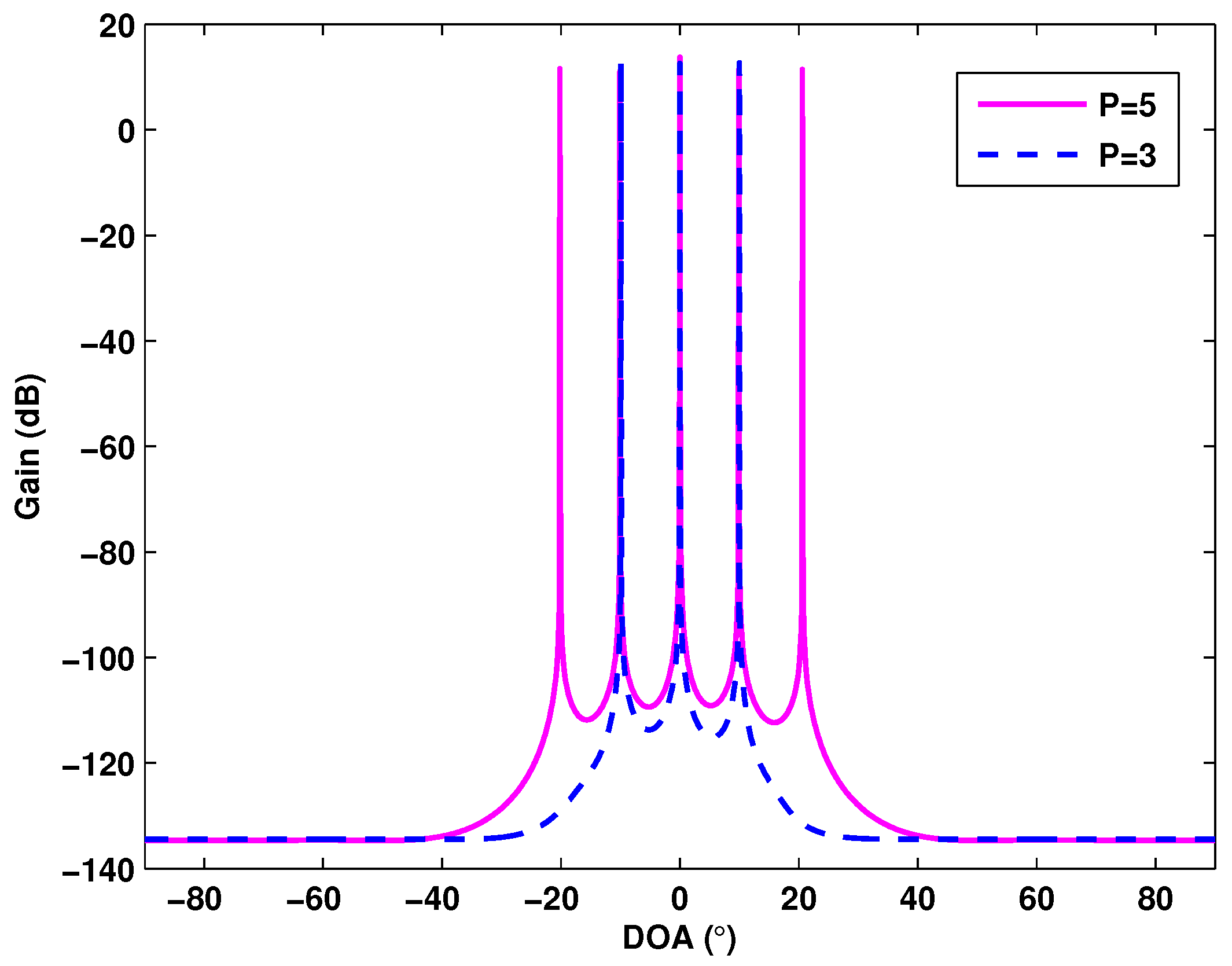
Figure 3 depicts the spatial spectrum of the proposed method for the number of targets being P = 3 and P = 5 , respectively, where M = N = 6 , J = 200 , SNR is fixed at SNR = 0 dB and mutual coupling Case (1) is considered. For P = 3 , the DOAs of the uncorrelated targets are θ 1 = 10 , θ 2 = 0 , θ 3 = 10 . For P = 5 , they are θ 1 = 20 , θ 1 = 10 , θ 1 = 0 , θ 2 = 10 and θ 3 = 20 , respectively. From Figure 3, it can be observed that the spatial spectrum peaks of the proposed method are sharp, and the sidelobe suppression is low. In addition, for different target numbers P, the spectrum maintains the accuracy of DOA estimation. This indicates that the proposed method is effective to perform DOA estimation accurately.
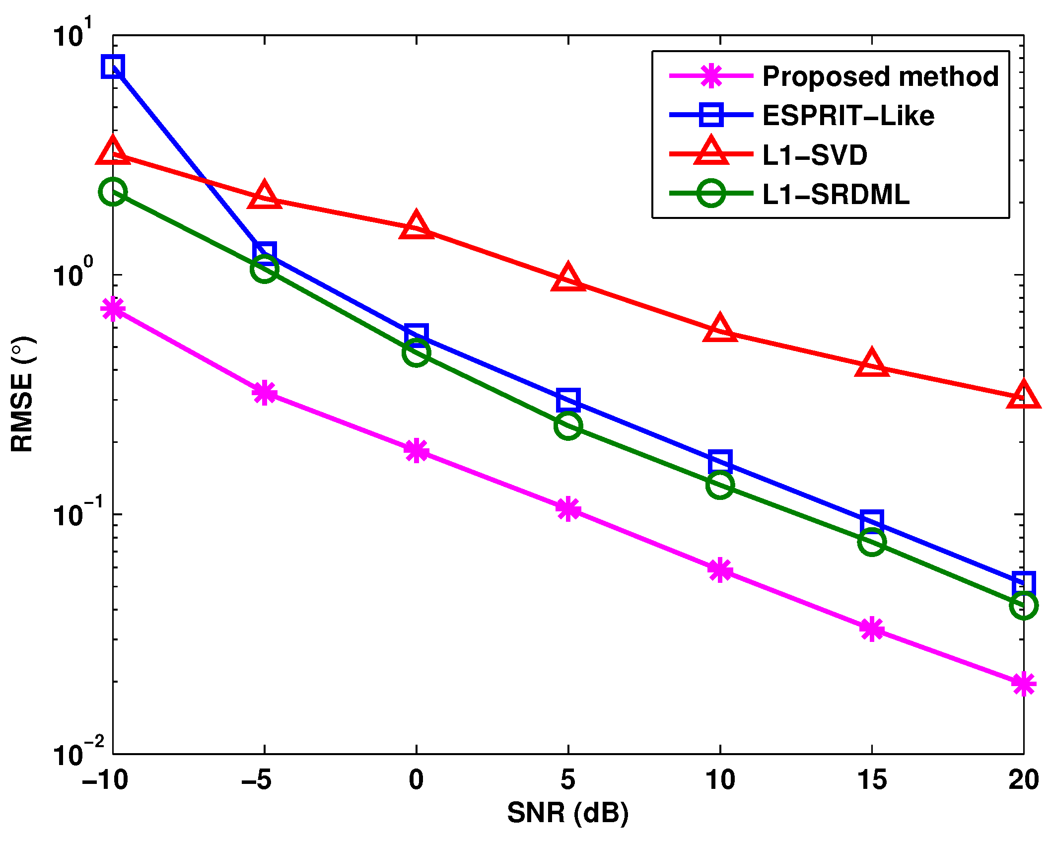
Figure 4 shows the RMSE of DOA estimation versus SNR in different methods with mutual coupling Case (1), where M = N = 6 , J = 200 and three targets with θ 1 = 10 , θ 2 = 0 , θ 3 = 10 are considered. Additionally, the values of RMSE are computed by Equation (26) with Q trials. As can be seen in Figure 4, l 1 -SRDML owns a lower RMSE than the ESPRIT-like and l 1 -SVD algorithms, because the deterministic maximum likelihood procedure improves the estimation accuracy. In addition, the proposed method provides the best DOA estimation performance in all SNR regions, for the reason that the noncircularity-based joint reweighted sparse representation scheme enlarges the virtual array aperture and enhances the sparse solution.
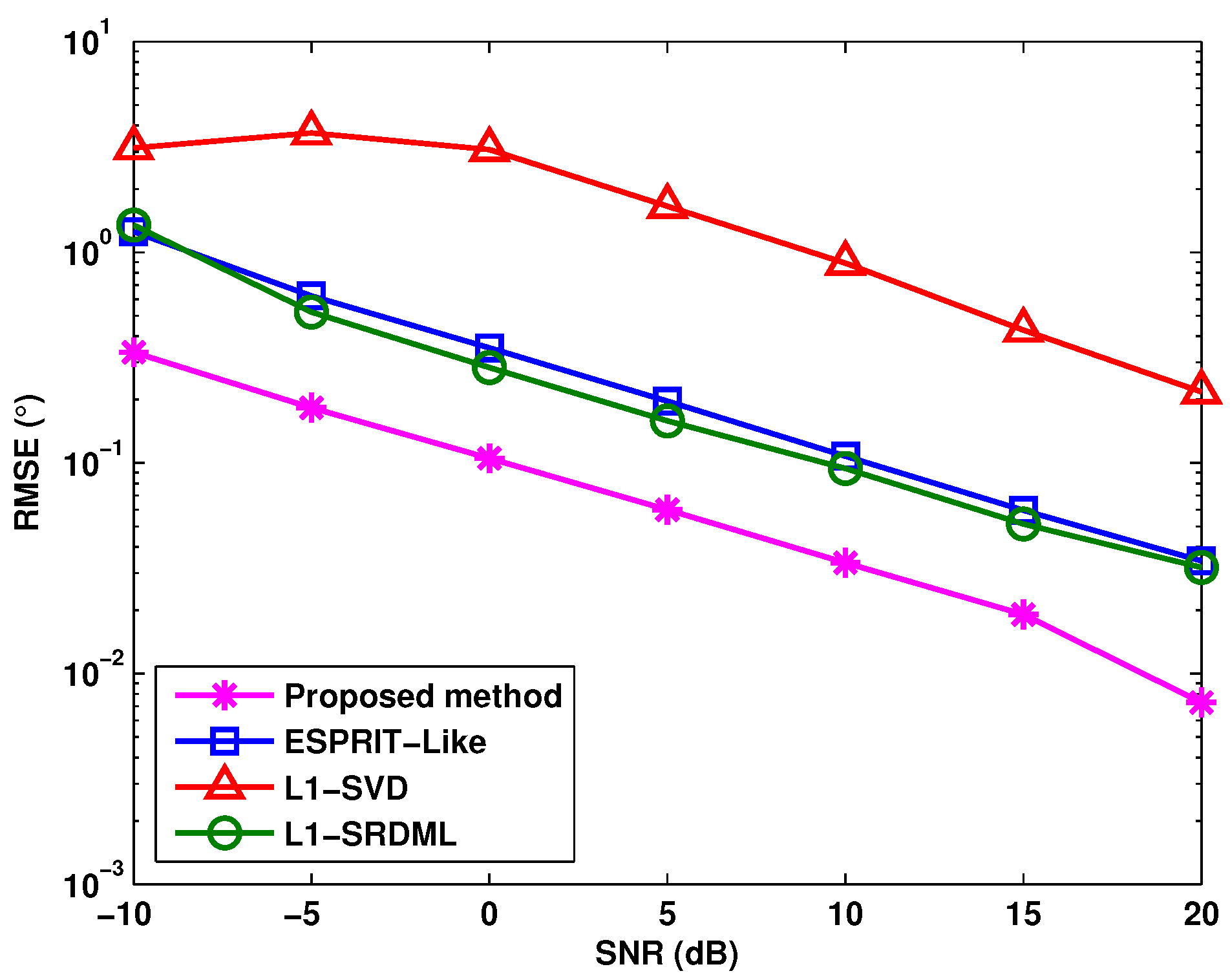
Figure 5 illustrates the RMSE of DOA estimation versus SNR in different methods with mutual coupling Case (2), where M = N = 7 , J = 200 , and there are three uncorrelated targets located at θ 1 = 15 , θ 2 = 0 , θ 3 = 15 . From Figure 5, it is clear that the performance of l 1 -SVD is inferior to the other algorithms, and the proposed method has the lowest RMSE in all analyzed methods. This means that when the number of nonzero mutual coupling coefficients increases, the proposed method still has superior DOA estimation performance.
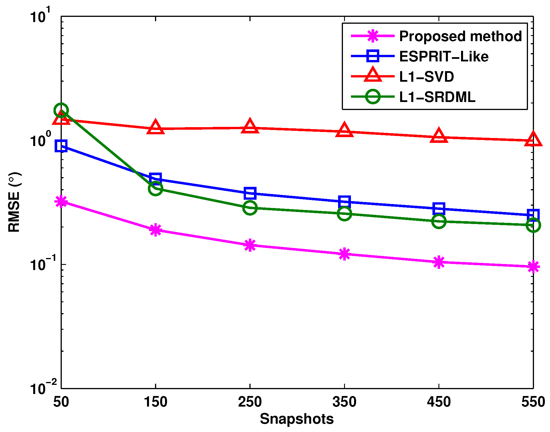
Figure 6 shows the RMSE of DOA estimation versus snapshots of different methods with mutual coupling Case (1), where M = N = 6 , SNR = 0 dB, there are three uncorrelated targets with DOAs being θ 1 = 11.5 , θ 2 = 0 , θ 3 = 11.5 and the number of snapshots varies from J = 50 to J = 550 . It can be seen from Figure 6 that the proposed method performs well in the case of fewer snapshots, and with obvious superiority over the ESPRIT-like, l 1 -SVD and l 1 -SRDML algorithms, the proposed method performs the best in all pf the ranges of snapshots on account of the application of the reweighted matrix and the noncircularity of emitted signals.
Figure 7 demonstrates the target resolution probability of different methods versus SNR with mutual coupling Case (1), where M = N = 6 , J = 100 and the DOAs of three targets are θ 1 = 20 , θ 2 = 0 and θ 3 = 20 , respectively. They can be regarded as successfully detected when all of their absolute DOA estimation errors are within 0.1 . It can be observed that when SNR is high enough, all methods provide 100 % target resolution probability. Owing to the increased number of virtual array elements, more diversity gain is obtained in the proposed algorithm. Consequently, the proposed method provides higher resolution probability than the ESPRIT-like, l 1 -SVD and l 1 -SRDML algorithms in all SNR regions, as shown in the simulation results of Figure 7.

6. Conclusions

In this paper, we have proposed the noncircular source-based sparse representation algorithm for DOA estimation in MIMO radar with mutual coupling. On the basis of the error matrix structure and the properties of noncircular signals, the proposed method eliminates the effect of mutual coupling and obtains the extended observation matrix. Then, the joint reweighted sparse representation scheme is constructed to achieve the DOA estimation. The computational complexity of the proposed method has been analyzed, and the simulation results have verified that in the presence of mutual coupling, the proposed algorithm provides higher resolution and better angle estimation performance than the ESPRIT-like, l 1 -SVD and l 1 -SRDML algorithms.

Acknowledgments

This work was supported by the China Scholarship Council and the Fundamental Research Funds for the Central Universities (HEUCF160401).

Author Contributions

Weidong Zhou and Jing Liu contributed to the new method and completed this paper. Pengxiang Zhu, Wenhe Gong and Jiaxin Hou assisted in performing the simulation experiments and analyzing the results.

Conflicts of Interest

The authors declare no conflict of interest.

References

  1. Fishler, E.; Haimovich, A.; Blum, R. Performance of MIMO radar systems: Advantages of angular diversity. In Proceedings of the Thirty-Eighth Asilomar Conference on Signals, Systems and Computers, Pacific Grove, CA, USA, 7–10 November 2004; pp. 305–309.
  2. Wang, X.; Jeske, D.; Serpedin, E. An overview of a class of clock synchronization algorithms for wireless sensor networks: A statistical signal processing perspective. Algorithms 2015, 8, 590–620. [Google Scholar] [CrossRef]
  3. Gao, X.; Zhang, X.F.; Feng, G.P.; Wang, Z.Q.; Xu, D.Z. On the MUSIC-derived aprroaches of angle estimation for bistatic MIMO radar. In Proceedings of the 2009 International Conference on Wireless Networks and Information Systems, TBD, Shanghai, China, 28–29 December 2009; pp. 343–346.
  4. Chen, D.; Chen, B.; Qin, G. Angle estimation using ESPRIT in MIMO radar. Electron. Lett. 2008, 44, 770–771. [Google Scholar]
  5. Zhang, X.; Huang, Y.; Chen, C.; Li, J.; Xu, D. Reduced-complexity Capon for derection of arrival estimation in a monostatic mutiple-input multiple-output radar. IET Radar Sonar Navig. 2012, 8, 796–801. [Google Scholar] [CrossRef]
  6. He, J.; Gao, M.W.; Zhang, L.; Wu, H. Sparse signal recovery from fixed low-rank subspace via compressive measurement. Algorithms 2013, 6, 871–882. [Google Scholar] [CrossRef]
  7. Burns, B.L.; Wilson, N.E.; Thomas, M.A. Group sparse reconstruction of multi-dimensional spectroscopic imaging in human brain in vivo. Algorithms 2014, 7, 276–294. [Google Scholar] [CrossRef]
  8. Liu, Y.J.; Tao, T.Y. A CS recovery algorithm for model and time delay identification of MISO-FIR systems. Algorithms 2015, 8, 743–753. [Google Scholar] [CrossRef]
  9. Malioutov, D.; Cetin, M.; Willsky, A.S. A sparse signal reconstruction perspective for source localization with sensor arrays. IEEE Trans. Signal Process. 2005, 53, 3010–3022. [Google Scholar] [CrossRef]
  10. Yin, J.; Chen, T. Direction-of-arrival estimation using a sparse representation of array covariance vectors. IEEE Trans. Signal Process. 2011, 59, 4489–4493. [Google Scholar] [CrossRef]
  11. Wang, X.P.; Wang, W.; Li, X.; Liu, J. Real-valued covariance vector sparsity-inducing DOA estimation for monostatic MIMO radar. Sensors 2015, 15, 28271–28286. [Google Scholar] [CrossRef] [PubMed]
  12. Dai, J.; Xu, X.; Zhao, D. Direction-of-arrival estimation via real-valued sparse representation. IEEE Antennas Wirel. Propag. Lett. 2013, 12, 376–379. [Google Scholar] [CrossRef]
  13. Liu, X.; Liao, G. Direction finding and mutual coupling estimation for bistatic MIMO radar. Signal Process. 2012, 92, 517–522. [Google Scholar] [CrossRef]
  14. Zheng, Z.D.; Zhang, J.; Zhang, J.Y. Joint DOD and DOA estimation of bistatic MIMO radar in the presence of unknown mutual coupling. Signal Process. 2012, 92, 3039–3048. [Google Scholar] [CrossRef]
  15. Dai, J.; Zhao, D.; Ji, X. A sparse representation method for DOA estimation with unknown mutual coupling. IEEE Antennas Wirel. Propag. Lett. 2012, 11, 1210–1213. [Google Scholar] [CrossRef]
  16. Liu, J.; Wang, X.P.; Zhou, W.D. Covariance vector sparsity-aware DOA estimation for monostatic MIMO radar with unknown mutual coupling. Signal Process. 2016, 119, 21–27. [Google Scholar] [CrossRef]
  17. Bencheikh, M.L.; Wang, Y. Non circular ESPRIT-RootMUSIC joint DOA-DOD estimation in bistatic MIMO radar. In Proceedings of the 2011 7th International Workshop on Systems, Signal Processing and Their Applications (WOSSPA), Tipaza, Algeria, 9–11 May 2011; pp. 51–54.
  18. Picinbono, B. On circularity. IEEE Trans. Signal Process. 1994, 42, 3473–3482. [Google Scholar] [CrossRef]
  19. Yang, M.L.; Chen, B.X.; Yang, X.Y. Conjugate ESPRIT algorithm for bistatic MIMO radar. Electron. Lett. 2010, 46, 1692–1694. [Google Scholar] [CrossRef]
  20. Wang, W.; Wang, X.; Song, H.; Ma, Y. Conjugate ESPRIT for DOA estimation in monostatic MIMO radar. Signal Process. 2013, 93, 2070–2075. [Google Scholar] [CrossRef]
  21. Li, J.; Stoica, P. MIMO radar with colocated antennas. IEEE Signal Process. Mag. 2007, 24, 106–114. [Google Scholar] [CrossRef]
  22. Wang, W.J.; Ren, S.W.; Ding, Y.T.; Wang, H.Y. An efficient algorithm for direction finding against unknown mutual coupling. Sensors 2014, 14, 20064–20077. [Google Scholar] [CrossRef] [PubMed]
  23. Wang, Y.X.; Trinkle, M.; Ng, B.W.-H. DOA estimation under unknown mutual coupling and multipath with improved effective array aperture. Sensors 2015, 15, 30856–30869. [Google Scholar] [CrossRef] [PubMed]
  24. Friedlander, B.; Weiss, A.J. Direction finding in the presence of mutual coupling. IEEE Trans. Antenn. Propag. 1991, 39, 273–284. [Google Scholar] [CrossRef]
  25. Haardt, M.; Romer, F. Enhancements of unitary ESPRIT for non-circular sources. In Proceedings of the IEEE International Conference on Acoustics, Speech and Signal Processing, Montreal, QC, Canada, 17–21 May 2004; pp. 1520–6149.
  26. Abeida, H.; Delmas, J.P. MUSIC-like estimation of direction of arrival for noncircular sour. IEEE Trans. Signal Process. 2006, 54, 2678–2690. [Google Scholar] [CrossRef]
  27. Sturm, J.F. Using SeDuMi, A Matlab toolbox for optimization ove symmetric cones. Optim. Method Softw. 2009, 11–12, 625–653. [Google Scholar]
  28. Grant, M.; Boyd, S. CVX: MATLAB Software for Disciplined Convex Programming, Version 2.1; CVX Research: Austin, TX, USA, 2012.
  29. Taboga, M. Lectures on Probability Theory and Mathematical Statistics; Amazon CreateSpace: North Charleston, SC, USA, 2012; pp. 469–473. [Google Scholar]
  30. Wax, M.; Kailath, T. Detection of signals by information theoretic criteria. IEEE Trans. Acoust. Speech Signal Process. 1985, 33, 387–392. [Google Scholar] [CrossRef]
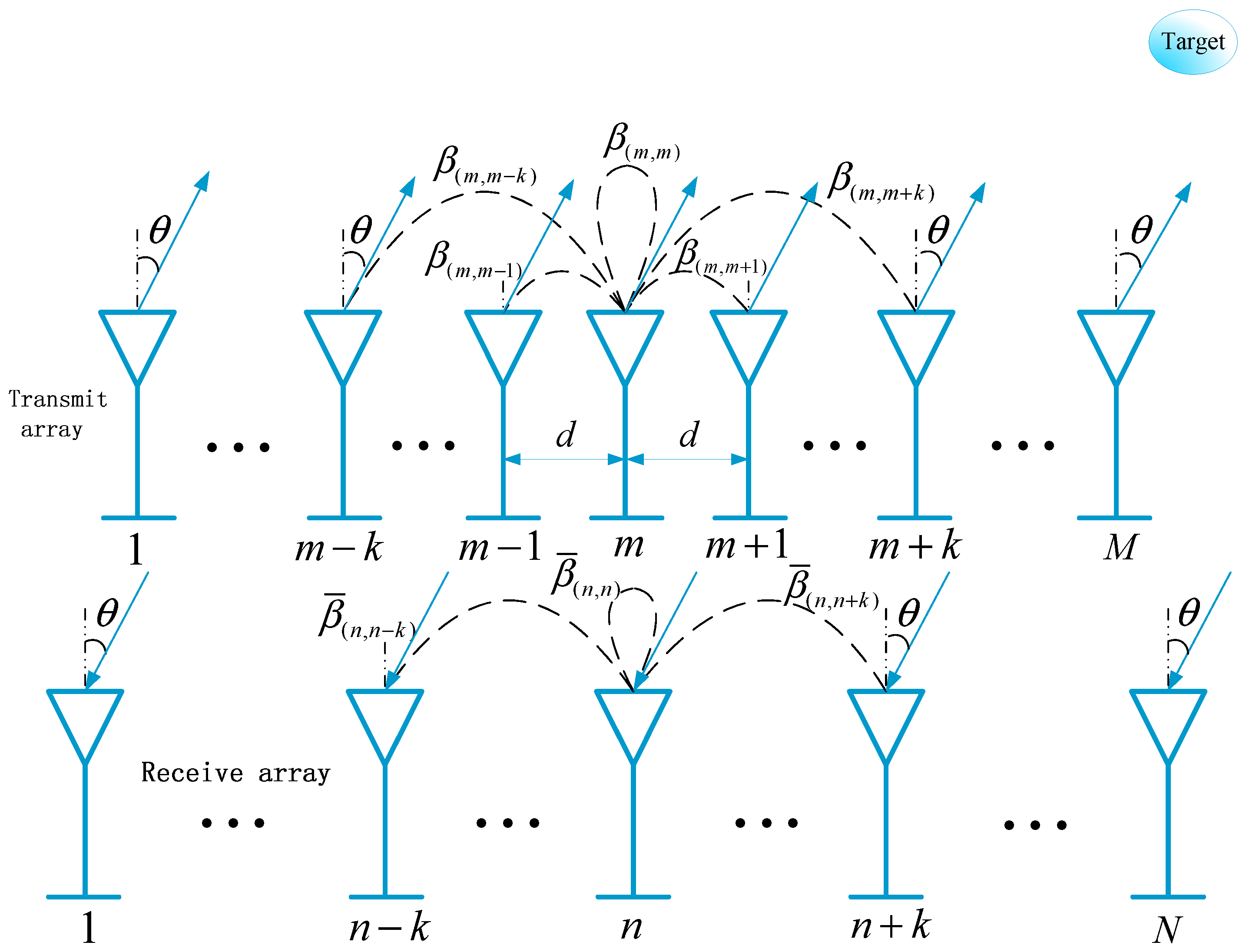
Figure 1. Configuration of MIMO radar in the presence of mutual coupling.
Algorithms 09 00061 g001
Figure 2. Difference between monostatic MIMO radar and bistatic MIMO radar.
Algorithms 09 00061 g002
Figure 3. Spatial spectrum of the proposed method with target number P = 3 and P = 5 .
Algorithms 09 00061 g003
Figure 4. RMSE versus SNR in ESPRIT-like, l 1 -SVD and l 1 -SRDML (sparse representation deterministic maximum likelihood) methods for nonzero mutual coupling coefficient number K = 2 .
Algorithms 09 00061 g004
Figure 5. RMSE versus SNR in the ESPRIT-like, l 1 -SVD and l 1 -SRDML methods for nonzero mutual coupling coefficient number K = 3 .
Algorithms 09 00061 g005
Figure 6. RMSE versus snapshots in the ESPRIT-like, l 1 -SVD and l 1 -SRDML methods when SNR = 0 dB.
Algorithms 09 00061 g006
Figure 7. Target resolution probability versus SNR in the ESPRIT-like, l 1 -SVD and l 1 -SRDML methods with snapshot number J = 100 .
Algorithms 09 00061 g007