Multiple Artificial Neural Networks with Interaction Noise for Estimation of Spatial Categorical Variables

Abstract

This paper presents a multiple artificial neural networks (MANN) method with interaction noise for estimating the occurrence probabilities of different classes at any site in space. The MANN consists of several independent artificial neural networks, the number of which is determined by the neighbors around the target location. In the proposed algorithm, the conditional or pre-posterior (multi-point) probabilities are viewed as output nodes, which can be estimated by weighted combinations of input nodes: two-point transition probabilities. The occurrence probability of a certain class at a certain location can be easily computed by the product of output probabilities using Bayes’ theorem. Spatial interaction or redundancy information can be measured in the form of interaction noises. Prediction results show that the method of MANN with interaction noise has a higher classification accuracy than the traditional Markov chain random fields (MCRF) model and can successfully preserve small-scale features.

1. Introduction

Categorical spatial data, such as area-class maps and remote sensing images, are very common and important information sources in geographic information science [1]. Many approaches have been developed to model the uncertainty in categorical random fields, including but not limited to Markov chain random fields (MCRF) [2,3], the multinomial logistic mixed model [4], the spatial hidden Markov chain [5] and the Bayesian updating model [6]. Artificial neural networks (ANNs) [7] have also been extensively used as non-linear and semi-parametric pattern classifiers and function estimators (e.g., classification and regression tools) in geographical information systems and regional science since the 1990s [8,9,10,11]. Civco [12] described the application of ANNs to the problem of deriving land-cover information from Landsat satellite Thematic Mapper digital imagery. Skabar [13] reported on the application of ANNs to mapping reef gold mineralization potential and showed that the ability of ANNs to predict the presence of hold-out test deposits is significantly better than that for logistic regression. Conceptually, ANNs are well suited to processing noisy data and handling non-linear modeling tasks [14], and they seem to offer methodological advantages over traditional spatial analysis methods in that ANNs contain no critical assumptions about the nature of spatial data. The analysis of a priori knowledge and data on known physical constraints can also be incorporated into ANNs’ interpolation process [15,16], while traditional interpolation methods such as kriging seem to lack of the flexibility to incorporate important general and case-specific sources.

The idea of our multiple artificial neural networks (MANN) model with interaction noise is to apply a linear function to the input nodes, i.e., transition probabilities (two-point), and regard the pre-posterior probabilities (multi-point) as derived features via nonlinear transformation. We need to construct multiple ANNs to obtain the target multi-point posterior probabilities by employing Bayes’ theorem. The interaction noises are used for estimating the multi-point pre-posterior probabilities in the MANN training processes. The originality of the proposed solution lies in that no additional assumptions are made about the relationship between the multi-point pre-posterior probabilities and two-point transition probabilities, which takes a step forward with respect to the existing methods. In addition, we have also proposed a method for measuring the spatial interaction effects. The remainder of this paper is organized as follows. We give an overview and formulate the method of MANN with interaction noise in Section 2. To demonstrate our model, an artificial and a real-word case study have been carried out in Section 3. Conclusions and directions for future research are presented in Section 4.

2. Method

Consider a categorical random variable (RV) $C\left(x_0\right)$ which can take one out of $K$ mutually exclusive and collectively exhaustive states $c(x_0)\in \left\{1,\cdots ,K\right\}$ at any arbitrary location with coordinate $x_0$; when there is no other information, we assume that the probability mass function (PMF) of RV $C\left(x_0\right)$ is stationary and can be approximated by the $K$ global class proportions ${\pi }_1,\cdots ,{\pi }_K$. A central task in prediction and simulation of categorical random fields is the estimation of the conditional PMF of $C\left(x_0\right)$ in the presence of observed class labels $c\left(x_1\right),\cdots ,c\left(x_N\right)$ available at $N$ locations $x_1,\cdots ,x_N$. Our task can now be re-stated as that of estimating the conditional PMF $P\left\{C\left(x_0\right)|c\left(x_1\right),\cdots ,c\left(x_N\right)\right\}$. To simplify notation, we use $A$ and $D_1,\cdots ,D_N$ to represent the events in sample spaces of $C\left(x_0\right)$ and $C\left(x_1\right),\cdots ,C\left(x_N\right)$, respectively, and $\overline{A}$ to denote the complementary event of $A$. ANNs offer an approach to geostatistical simulation with the possibility of automatic recognition of the correlation structure. We consider $f_i=P\left(D_j|A\right),j\in \left\{1,2,\cdots ,i\right\}$ as the input node, and thus the pre-posterior (multi-point) probabilities $y_i=P\left(D_i|A{D}_1\cdots D_{i-1}\right),i=2,\cdots ,N$ can be regarded as the desired output node. To obtain the target (multi-point) posterior probability $P\left(A|D_1{D}_2\cdots D_N\right)$, we need to train $N-1$ ANNs, which is called the MANN.

The continuously differentiable sigmoid functions are the most common form of activation function in ANNs [17], and the learning process is achieved by using feed forward and back propagation algorithms. Let ${\widehat{y}}_i=\widehat{P}\left(D_i|A{D}_1\cdots D_{i-1}\right)$ be the actual output obtained on one particular iteration after $f_i$ has been fed forward through the network. The current total error, which is defined as a function of the connection weights, is:

$$E\left(W\right)={{\displaystyle {\sum }_{i=2}^N\left(y_i-\widehat{y}{}_i\right)}}^2$$

(1)

where $W$ is the matrix of connection weights.

In most traditional neural networks, the desired output nodes are considered as known response variables. Thus, the central work of an ANN is to train the appropriate weights in hidden layers. However, the desired outputs $y_i=P\left(D_i|A{D}_1\cdots D_{i-1}\right),i=2,\cdots ,N$ in our model cannot be obtained from the available training set directly. We use MANN with interaction noise to solve this problem. Just as MCRF, Tau $(\tau )$ model [18] and Nu $(\upsilon )$ expression [19] suggested, $P\left(D_i|A{D}_1\cdots D_{i-1}\right)$ is primarily determined by $P\left(D_i|A\right)$. We assume that

$$\ln \frac{P\left(D_i|A{D}_1\cdots D_{i-1}\right)}{P\left(D_i|A\right)}={\epsilon }_i$$

(2)

where $\ln$ denotes the natural logarithm, ${\epsilon }_i$ is a random noise which capsules the interaction information from $D_1$ to $D_i$. Spearman correlation coefficients are used to measure the interdependence from $P\left(D_1|A\right)$ to $P\left(D_i|A\right)$. In this method, the one that has the most significant correlation with $P\left(D_i|A\right)$ is chosen to be the input node.

Thus, a neural network can be represented in terms of nested transformations of linear combinations of input units, where the initial input units are the predictor variables themselves, so that the overall network function with $H$ hidden units and activation functions $\phi$ and $\psi$ becomes

$$P\left(D_i|A{D}_1\cdots D_{i-1}\right)=\psi \left\{{\displaystyle \sum _{h=0}^H{\omega }_h^{(2)}\phi \left[{\displaystyle \sum _{h=0}^H{\omega }_h^{(1)}P\left(D_j|A\right)}\right]}\right\},j\in \left\{1,2,\cdots i\right\},i=2,\cdots ,N$$

(3)

where ${\omega }_h^{\left(1\right)}$ and ${\omega }_h^{\left(2\right)}$ indicate the weights in the inner and outer layer, respectively, and the bias parameters are absorbed into the set of weight parameters by defining an additional input variable $P\left(D_0|A\right)$ whose value is clamped at $P\left(D_0|A\right)=1$. Using Bayes’ theorem (or the definition of conditional probability), we can decompose the conditional PMF as follows

$$\begin{array}{l}P\left\{C\left(x_0\right)=k|C\left(x_1\right)=l_1,\cdots ,C\left(x_N\right)=l_N\right\}\\ =P\left(A|D_1{D}_2\cdots D_N\right)\\ =\frac{P\left(D_1\right)P\left(A|D_1\right)P\left(D_2|A{D}_1\right)\cdots P\left(D_N|A{D}_1\cdots D_{N-1}\right)}{P\left(D_1{D}_2\cdots D_N\right)}\end{array}$$

(4)

where $x_1$ is the nearest neighbor of $x_0$ among the $N$ locations, $l_1,\cdots l_N\in \left\{1,2,\cdots ,K\right\}$. Therefore, we can compute the posterior occurrence probabilities of different classes according to Equation (4), and then estimate the category at the target location based on the “maximum a posterior” criterion. According to the above description, the proposed approach can be coded easily on the computer and the flowchart can be summarized as in Figure 1.

One of the commonly used methods to compute the multi-point posterior PMF is the MCRF model. The highlight of this theory is that there is only a single spatial Markov chain that moves (or jumps) in a space, which avoids the small-class underestimation problem in modeling the categorical random field [2]. Nevertheless, the multi-point probabilities $P\left(D_i|A{D}_1\cdots D_{i-1}\right)$, $i=2,3,\cdots ,N$ are difficult to calculate. Hence, the general solution of the MCRF model is deduced based on the conditional independence assumption, which is

$$P\left(D_i|A{D}_1\cdots D_{i-1}\right)=P\left(D_i|A\right),i=2,\cdots ,N$$

(5)

By plugging Equations (3) and (5) into Equation (4), the posterior PMF can be determined. Note that $P\left(A|D_1\right)$ is the two-point transition probability and can be estimated from paired samples. Additionally, $P\left(D_1\right)$ and $P\left(D_1{D}_2\cdots D_N\right)$ are the normalization constants and should be computed using the sum rule, since they do not contain the unknown event $A$.

3. Case Study

3.1. Synthetic Case Study

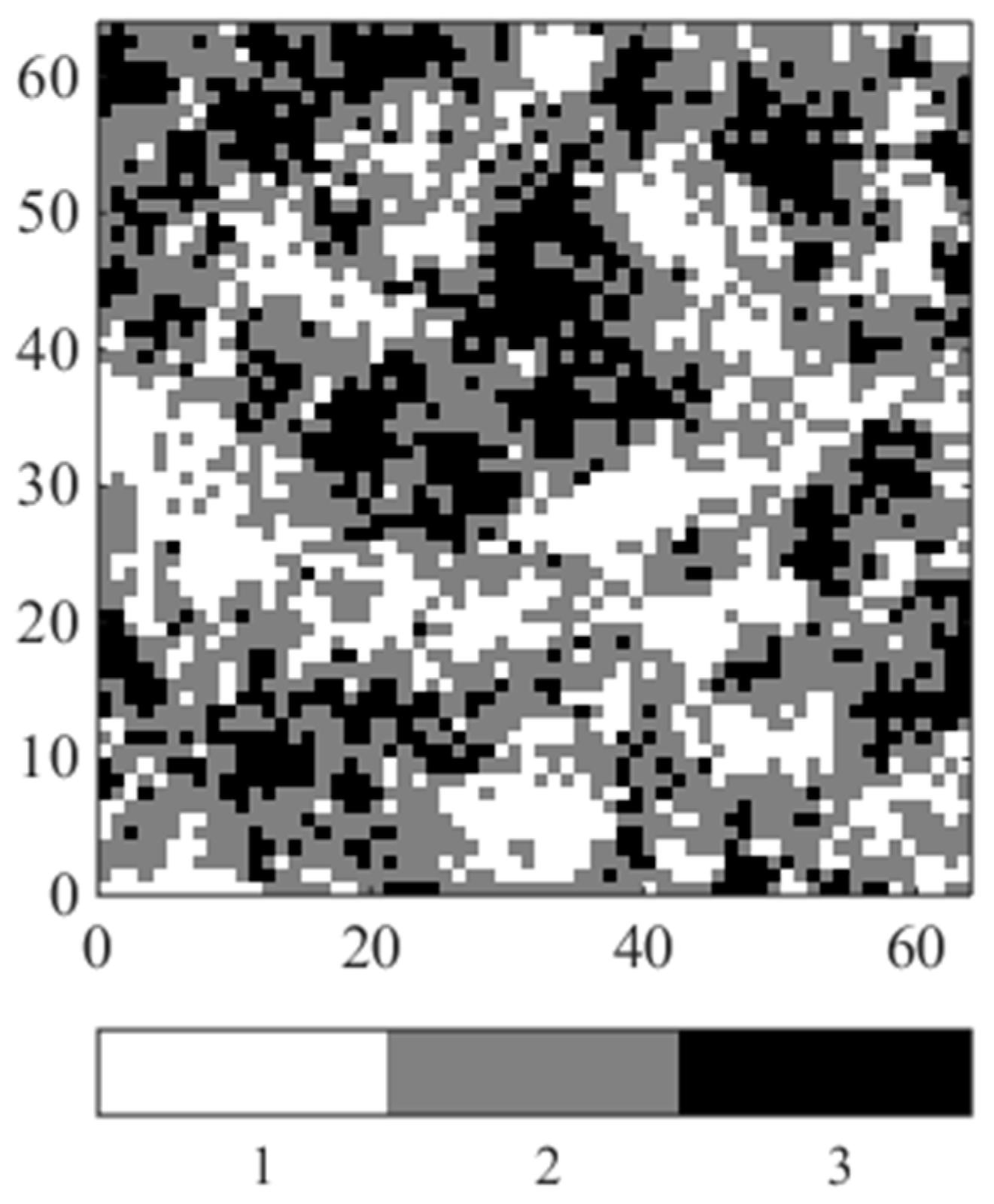
We first illustrate our method on a synthetic case study with three categories (Figure 2). There are 606 locations that have been randomly sampled from this image. The prediction is conducted over a 64 × 64 grid covering the square. The marginal probability of the occurrence vector is (0.2756, 0.4653, 0.2591). The categories may represent geological facies, soil types, land uses or any other categorical variable [20].

As a first task, the data set is used to estimate the two-point input transition probabilities. Experimental transition probabilities can be directly estimated from paired sampling data by counting the transition frequencies of classes with different lags [21]. A continuous transiogram [22] can be obtained via interpolation [23] or fitting the transition probabilities cloud with various models. Following [6], the exponential model is employed for transiogram fitting. After all these preparations, the input vectors of the ANNs can be determined.

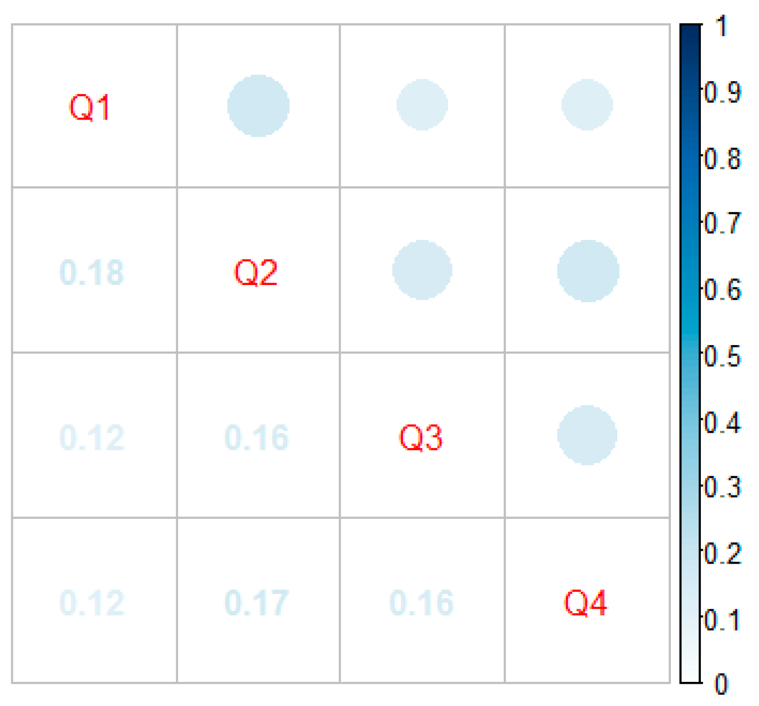
We consider the four nearest sampling points as the neighbors of the unknown location. To use Equation (3), we must train three compositional ANNs to compute the pre-posterior (multi-point) probabilities. The problem here is the choice of the input nodes. By analyzing the correlation plot (Figure 3) of these four transition probabilities, no significant correlation is found among the input vectors; therefore, we choose $P\left(D_i|A\right)$ as the input of $P\left(D_i|A{D}_1\cdots D_{i-1}\right)$, $i=2,3,4$, respectively.

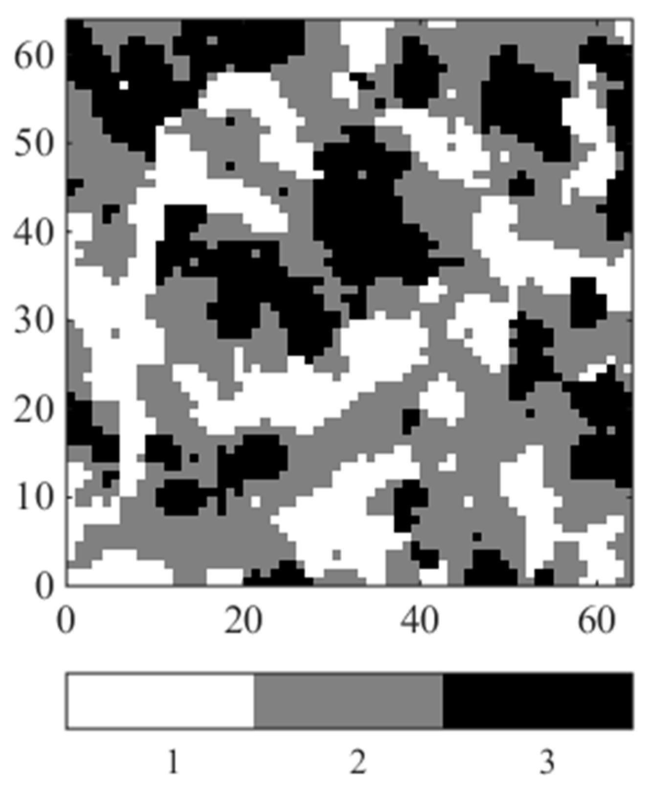
As a second task, the Gaussian-distributed interaction noises with different means and variances are simulated. For the 606 training data set, the output nodes $P\left(D_i|A{D}_1\cdots D_{i-1}\right)$ can be computed via Equation (2). For comparison purposes, we use 10 groups of parameters for estimating and simulating the spatial categorical data in the remaining 3490 locations. We find in

Table 1. Prediction accuracy comparison of the raster data set. $\mu$ and $\sigma$ denote the mean and standard deviation, respectively.

Parameters	Class 1	Class 2	Class 3	Total
$\mu =0$;$\sigma =0.1$	58.02% (579/998)	50.49% (830/1644)	60.97% (517/848)	55.19% (1926/3490)
$\mu =-1$;$\sigma =0.1$	58.62% (585/998)	50.67% (833/1644)	60.85% (516/848)	55.42% (1934/3490)
$\mu =-1$;$\sigma =0.5$	58.82% (587/998)	51.03% (839/1644)	60.02% (509/848)	55.44% (1935/3490)
$\mu =-2$;$\sigma =0.5$	57.72% (576/998)	52.86% (869/1644)	59.55% (505/848)	55.87% (1950/3490)
$\mu =-3$;$\sigma =0.9$	54.91% (548/998)	56.20% (924/1644)	57.90% (491/848)	56.25% (1963/3490)
$\mu =-3$;$\sigma =1.2$	55.71% (556/998)	55.90% (919/1644)	58.37% (495/848)	56.45% (1970/3490)
$\mu =-4$;$\sigma =1.2$	52.30% (522/998)	57.85% (951/1644)	56.60% (480/848)	55.96% (1953/3490)
$\mu =-4$;$\sigma =1.5$	53.51% (534/998)	57.24% (941/1644)	57.19% (485/848)	56.16% (1960/3490)
$\mu =-5$;$\sigma =1.2$	53.51% (518/998)	54.01% (888/1644)	57.08% (484/848)	54.15% (1890/3490)
$\mu =-5$;$\sigma =1.5$	50.00% (499/998)	55.41% (911/1644)	56.84% (482/848)	54.21% (1892/3490)
MCRF	57.21% (571/998)	51.64% (849/1644)	60.85% (516/848)	55.47% (1936/3490)

that when the parameters are specified by $\mu =-3$ and $\sigma =1.2$, the prediction has the highest overall classification accuracy with 56.45% (1970 out of 3490). From the interpolation map generated by MANN with interaction noise (Figure 4), we find that clear inter-class boundaries have been shaped and spatial patch patterns have been retained. To demonstrate the superiority in terms of accuracy, MCRF, as a competing method, has been used for comparison. This counterpart, however, only correctly classifies 1936 samples out of 3490 locations. Based on this result, MANN with interaction noise performs better than MCRF in terms of prediction accuracy in this artificial data set.

3.2. Real-World Case Study

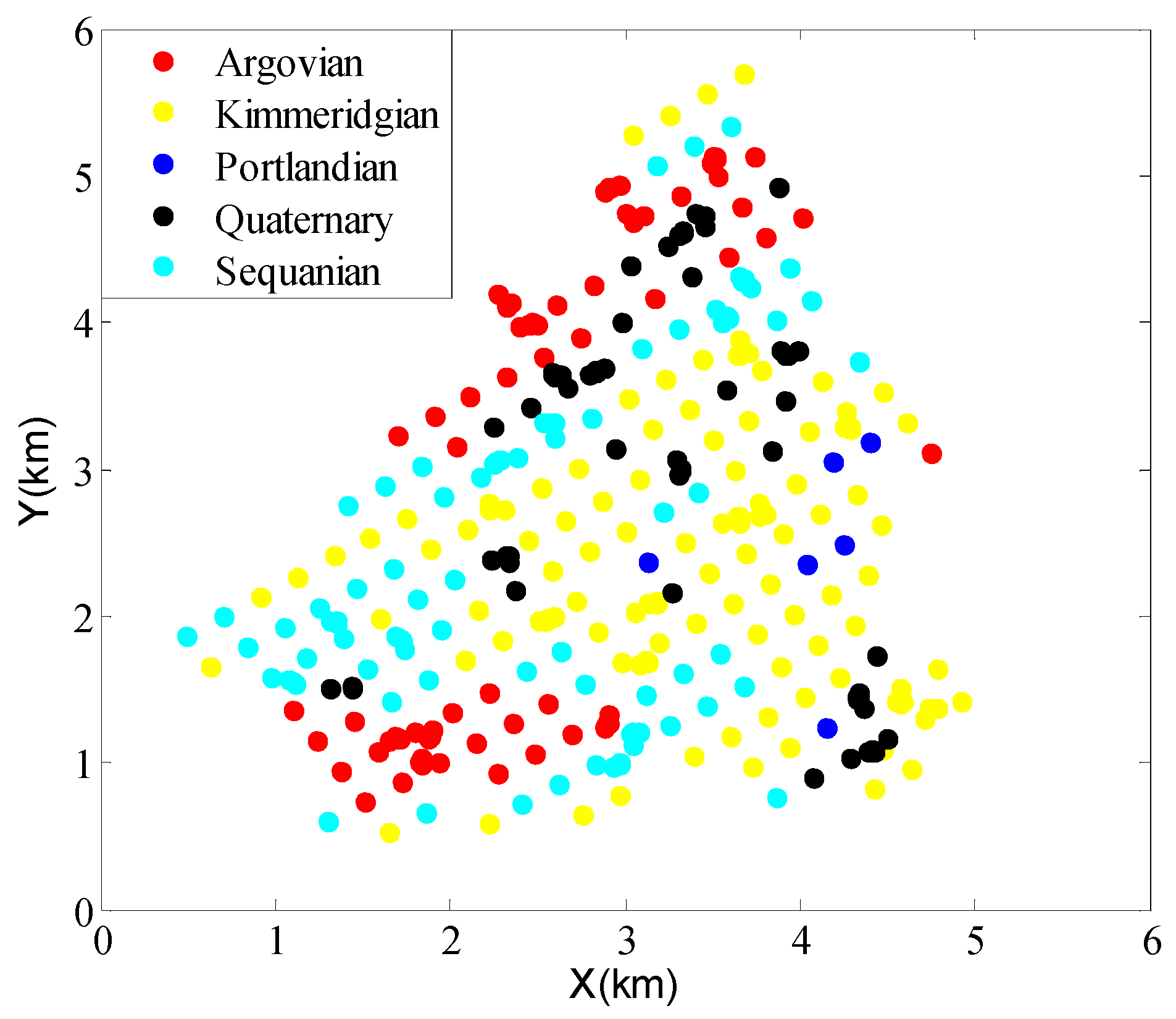
To further investigate the performance of the proposed method in real cases, the lithology types in the well-known Swiss Jura data set [24] are used, in which five rock types are sampled at 359 locations in a 14.5 km² area (Figure 5). The class proportions of these five categories are (0.2046, 0.3282, 0.2432, 0.0116, 0.2124), respectively. We focus on MANN with sigmoid activation functions and consider the 10 nearest samples as the neighbors of the target point. For the proposed method, we choose the one that has the maximum correlation with output probabilities as the input and we have trained nine compositional ANNs.

We furthermore assume that the random interaction noise $\epsilon =\left({\epsilon }_1,{\epsilon }_2,\cdots ,{\epsilon }_9\right)$ is a Gaussian random field. By trial and error, we find that the model which has the highest classification accuracy can be specified by mean $\mu =0$ and standard deviation $\sigma =0.1$; that is,

$$P\left({\epsilon }_i\right)=\mathrm{N}\left(0,0.01\right), \mathrm{cov}\left({\epsilon }_i,{\epsilon }_j\right)=0\text{ for }i\ne j.$$

(6)

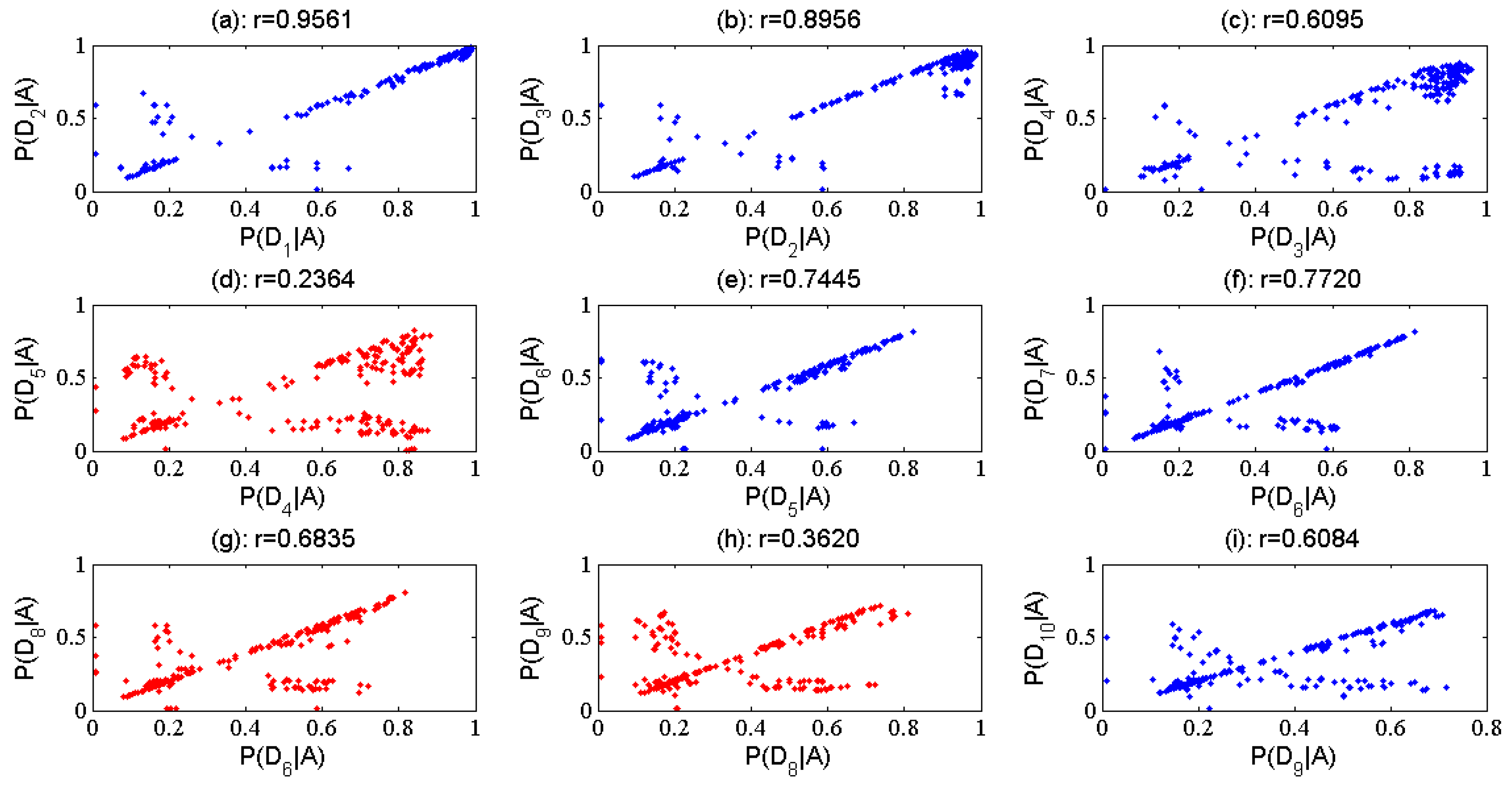
Correlation coefficients between various transition probabilities are compared with each other and the maximum correlation pairs are shown in Figure 6, where the red pictures (Figure 6d,h) are worthy of discussion. Note that the correlation between $P\left(D_4|A\right)$ and $P\left(D_5|A\right)$ is quite weak with $r=0.2364$, and the relevance from $P\left(D_1|A\right)$ to $P\left(D_3|A\right)$ with $P\left(D_5|A\right)$ is even lower. In such a case, we choose $P\left(D_5|A\right)$ itself as the input node of $P\left(D_5|A{D}_1\cdots D_4\right)$, since no significant interaction information is found from $D_1$ to $D_5$. In the same way, $P\left(D_9|A\right)$ is considered as the input node of $P\left(D_9|A{D}_1\cdots D_8\right)$. It is rather remarkable that the maximum correlation pairs may not always be $P\left(D_i|A\right)$ and $P\left(D_{i-1}|A\right)$, just as Figure 6g displays. $P\left(D_6|A\right)$ rather than $P\left(D_7|A\right)$ is chosen as the input node for output $P\left(D_8|A{D}_1\cdots D_7\right)$, which means that the main interaction information among $D_1,D_2,\cdots D_8$ is encapsulated in $D_6$ and $D_8$. In general, the input nodes of $P\left(D_i|A{D}_1\cdots D_{i-1}\right)$, $i=2,3,\cdots ,10$, should be $P\left(D_{i-1}|A\right)$ if the correlation coefficients between $P\left(D_{i-1}|A\right)$ and $P\left(D_i|A\right)$ exceed 0.5. The R package “nnet” designed under the framework of feed forward and back propagation algorithms is used during the training process. We consider three units in the hidden layer. The training weights of MANN with interaction noise are given in

Table 2. Training weights of MANN with interaction noise. Input node, hidden nodes and output node are represented by i, h1 to h3 and o, respectively; b1 and b2 are the bias nodes in the hidden layers.

Nodes	Weights
	ANN1	ANN2	ANN3	ANN4	ANN5	ANN6	ANN7	ANN8	ANN9
b1->h1	0.11	−3.74	−2.15	−0.15	−0.11	5.61	−0.05	0.23	0.03
i->h1	0.66	5.64	2.54	−6.28	2.04	−7.38	1.97	−2.48	−0.54
b1->h2	0.03	0.65	−0.53	0.29	4.02	0.56	6.08	0.24	0.53
i->h2	0.14	0.52	1.08	−1.02	−4.93	2.65	−7.00	−2.48	−0.42
b1->h3	−5.43	0.66	1.04	−3.16	0.60	0.09	0.28	0.24	2.73
i->h3	6.00	10.09	−1.58	3.85	12.06	0.13	0.80	−2.48	−5.02
b2->o	−0.49	2.31	−0.70	−0.21	4.87	0.91	1.42	2.33	0.55
h1->o	−0.75	4.81	3.05	−4.61	4.83	−4.12	2.18	−2.87	0.62
h2->o	−0.24	1.71	1.18	−1.24	−3.58	2.25	−4.72	−2.87	0.60
h3->o	6.76	−5.56	−2.32	4.12	−5.68	0.47	1.30	−2.87	-2.91

.

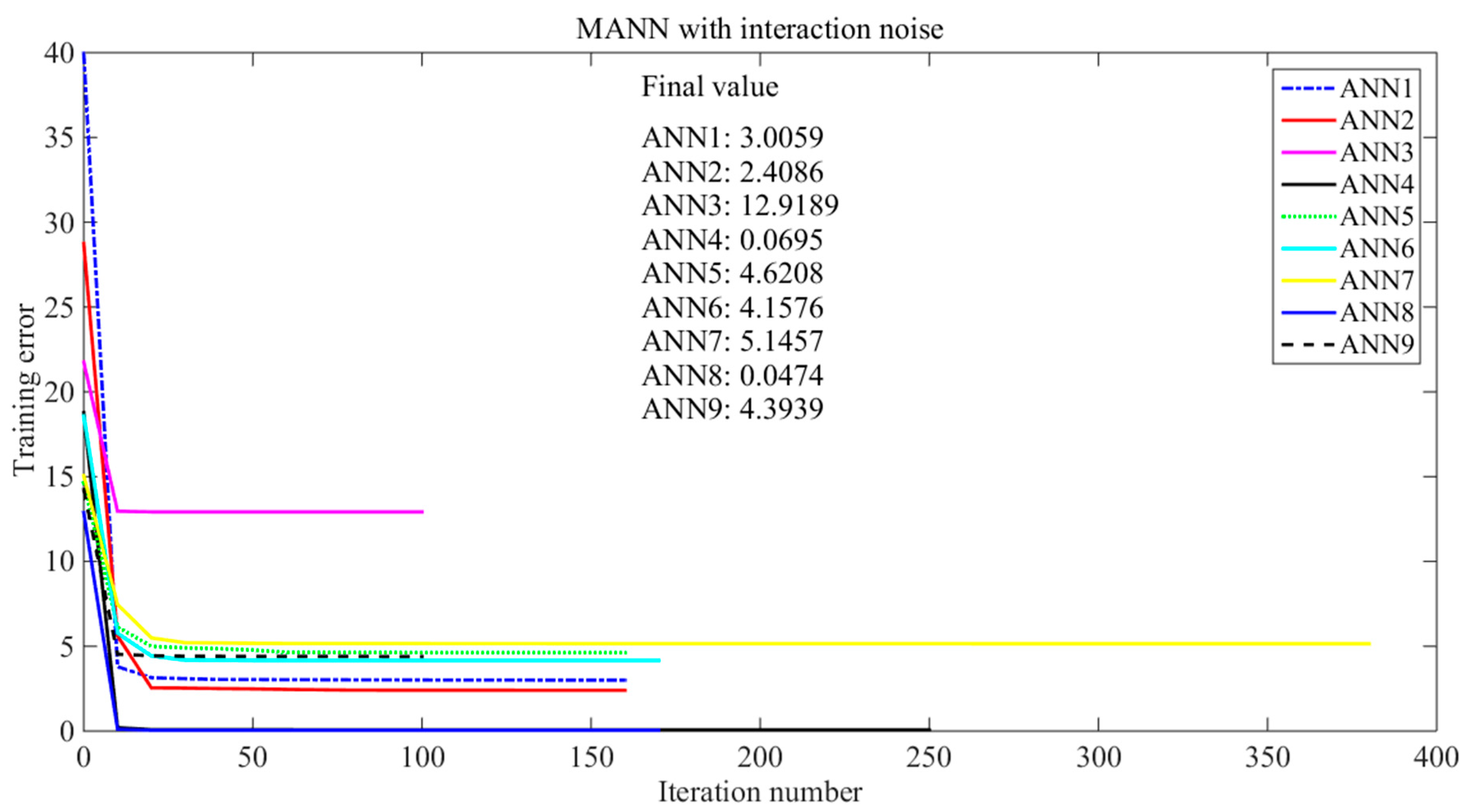
As can be seen from Figure 7, the nine ANNs converge after a certain number of iterations. The training error of MANN with interaction noise can be viewed as the summation of the nine ANNs, which is illustrated in Figure 7 by different colors and line styles. Our original image (Figure 8a) is obtained from the “jura.grid” data set kindly provided by R software 3.2.5, and the known 5957 grid values are used as the validation set. We find that MANN with interaction noise has a classification accuracy of 65.12% (3879 out of 5957) and can successfully preserve small-scale Quaternary patch features (Figure 8b). We have also used the MCRF method for comparison. Not surprisingly, the latter yields a relatively lower classification accuracy not only in overall prediction, but also in most of the single categories (

Table 3. Prediction accuracy comparison of the Jura data set.

Method	Argovian	Kimmeridgian	Sequanian	Portlandian	Quaternary	Total
MANN with interaction noise	75.78% (898/1185)	78.19% (1592/2036)	64.07% (1043/1628)	0.00% (0/316)	43.69% (346/792)	65.12% (3879/5957)
MCRF	72.07% (854/1185)	74.17% (1510/2036)	61.61% (1003/1628)	0.00% (0/316)	47.60% (377/792)	62.85% (3744/5957)

). This result is comprehensible, since the general solution of MCRF is based on the conditional independence assumption, which fails to measure the interaction or redundancy information among the neighboring sources. The important knowledge, however, has been successfully incorporated in the form of interaction noise in the proposed MANN model.

4. Conclusions

In this paper, a new prediction/interpolation algorithm, MANN with interaction noise, is proposed for modeling and reproducing spatial patterns in categorical random fields. Connection weights can be estimated in the framework of the feed forward and back propagation method. Our algorithm is imposed by some form of Gauss assumption, which is suitable in most general situations. Prediction results show that MANN with interaction noise has a higher classification accuracy than the conditional independence-based MCRF method and can successfully preserve small-scale features. However, the proposed model cannot exactly estimate the small class proportion (category four: Portlandian) in the Jura data set. This undesirable phenomenon is caused by the excessively sparse samples. Following [25], category four (Portlandian) was recategorized as five (Quaternary) by the authors of [4,6] since there are only three sample points within this category. Our experimental results confirm that this combination is necessary.

The most important step in the MANN framework is the estimation of the pre-posterior multi-point probabilities for the training procedure. In this work, this problem is solved by imposing exponential Gauss noise to the available two-point transition probabilities. Future research directions may include but not be limited to the scanning approach, which is similar to multi-point statistics [26] originating from petroleum geostatistics. The discussions with respect to these two parallel methods will be the topic of our upcoming studies.

References

1. Cao, G. Modeling uncertainty in categorical fields. In International Encyclopedia of Geography; Richardson, D., Ed.; Wiley-Blackwell: Malden, MA, USA, 2016; in press. [Google Scholar]
2. Li, W. Markov chain random fields for estimation of categorical variables. Math. Geol. 2007, 39, 321–335. [Google Scholar] [CrossRef]
3. Huang, X.; Wang, Z.; Guo, J. Theoretical generalization of Markov chain random field from potential function perspective. J. Cent. South Univ. 2016, 23, 189–200. [Google Scholar] [CrossRef]
4. Cao, G.; Kyriakidis, P.C.; Goodchild, M.F. A multinomial logistic mixed model for the prediction of categorical spatial data. Int. J. Geogr. Inf. Sci. 2011, 25, 2071–2086. [Google Scholar] [CrossRef]
5. Huang, X.; Li, J.; Liang, Y.; Wang, Z.; Guo, J.; Jiao, P. Spatial hidden Markov chain models for estimation of petroleum reservoir categorical variables. J. Petrol. Explor. Prod. Technol. 2016, 1–12. [Google Scholar] [CrossRef]
6. Huang, X.; Wang, Z.; Guo, J. Prediction of categorical spatial data via Bayesian updating. Int. J. Geogr. Inf. Sci. 2016, 30, 1426–1449. [Google Scholar] [CrossRef]
7. Huang, Y. Advances in artificial neural networks-methodological development and application. Algorithms 2009, 2, 973–1007. [Google Scholar] [CrossRef]
8. Fischer, M.M. Learning in neural spatial interaction models: a statistical perspective. J. Geogr. Syst. 2002, 4, 287–299. [Google Scholar] [CrossRef]
9. Fischer, M.M. Neural networks: A class of flexible non-linear models for regression and classification. In Handbook of Research Methods and Applications in Economic Geography; Karlsson, C., Andersson, M., Norman, T., Eds.; Edward Elgar: Cheltenham, UK, 2015; pp. 172–192. [Google Scholar]
10. Fischer, M.M.; Leung, Y. A genetic-algorithms based evolutionary computational neural network for modelling spatial interaction data. Ann. Reg. Sci. 1998, 32, 437–458. [Google Scholar] [CrossRef]
11. Fischer, M.M.; Reismann, M.; Hlavackova-Schindler, K. Neural network modeling of constrained spatial interaction flows: Design, estimation, and performance issues. J. Reg. Sci. 2003, 43, 35–61. [Google Scholar] [CrossRef]
12. Civco, D.L. Artificial neural networks for land-cover classification and mapping. Int. J. Geogr. Inf. Sci. 1993, 7, 173–186. [Google Scholar] [CrossRef]
13. Skabar, A. Modeling the spatial distribution of mineral deposits using neural networks. Nat. Resour. Model. 2007, 20, 435–450. [Google Scholar] [CrossRef]
14. Openshaw, S.; Openshaw, C. Artificial Intelligence in Geography; Wiley: Chichester, UK, 1997. [Google Scholar]
15. Haykin, S. Neural Networks: A Comprehensive Foundation; Macmillan: New York, NY, USA, 1994. [Google Scholar]
16. Atkinson, P.M.; Tatnall, A.R.L. Introduction neural networks in remote sensing. Int. J. Remote Sens. 1997, 18, 699–709. [Google Scholar] [CrossRef]
17. Bishop, C.M. Patter Recognition and Machine Learning; Springer: Berlin/Heidelberger, Germany, 2006. [Google Scholar]
18. Krishnan, S. The Tau model for data redundancy and information combination in earth sciences: Theory and application. Math. Geosci. 2008, 40, 705–727. [Google Scholar] [CrossRef]
19. Polyakova, E.I.; Journel, A.G. The Nu expression for probabilistic data integration. Math. Geol. 2007, 39, 715–733. [Google Scholar] [CrossRef]
20. Allard, D.; D’Or, D.; Froidevaux, R. An efficient maximum entropy approach for categorical variable prediction. Eur. J. Soil Sci. 2011, 62, 381–393. [Google Scholar] [CrossRef]
21. Li, W.; Zhang, C. Application of transiograms to Markov chain simulation and spatial uncertainty assessment of land-cover classes. GISci. Remote Sens. 2005, 42, 297–319. [Google Scholar] [CrossRef]
22. Li, W. Transiogram: a spatial relationship measure for categorical data. Int. J. Geogr. Inf. Sci. 2006, 20, 693–699. [Google Scholar]
23. Li, W.; Zhang, C. Linear interpolation and joint model fitting of experimental transiograms for Markov chain simulation of categorical spatial variables. Int. J. Geogr. Inf. Sci. 2010, 24, 821–839. [Google Scholar] [CrossRef]
24. Goovaerts, P. Geostatistics for Natural Resources Evaluation; Oxford University Press: New York, NY, USA, 1997. [Google Scholar]
25. Bel, L.; Allard, D.; Laurent, J.M.; Cheddadi, R.; Bar-Hen, A. CART algorithm for spatial data: Application to environmental and ecological data. Comput. Stat. Data Anal. 2009, 53, 3082–3093. [Google Scholar] [CrossRef]
26. Strebelle, S. Conditional simulation of complex geological structures using multiple-point statistics. Math. Geol. 2002, 34, 1–21. [Google Scholar] [CrossRef]
Figure 1. Flowchart of the proposed method.
Algorithms 09 00056 g001
Figure 2. Reference map with dimension 64 × 64 and three categories.
Algorithms 09 00056 g002
Figure 3. Correlation plot between various transition probabilities. Q1, Q2, Q3 and Q4 denote P ( D 1 | A ) , P ( D 2 | A ) , P ( D 3 | A ) and P ( D 4 | A ) , respectively.
Algorithms 09 00056 g003
Figure 4. Prediction map generated by MANN with interaction noise.
Algorithms 09 00056 g004
Figure 5. Jura lithology data set with 359 samples.
Algorithms 09 00056 g005
Figure 6. Maximum correlation coefficients between various transition probabilities.
Algorithms 09 00056 g006
Figure 7. Training errors in the iteration process of MANN with interaction noise; different colors and line styles are used to distinguish the nine compositional ANNs.
Algorithms 09 00056 g007
Figure 8. (a) Original image obtained from R software data set (jura.grid); (b) Classification maps generated by MANN with interaction noise. Simulations are conditioned on 359 samples in Jura lithology data set, note the small Quaternary patches (visualized in black) neglected in (a) are successfully recovered in the result of the proposed method (b).
Algorithms 09 00056 g008