Article

Sign Function Based Sparse Adaptive Filtering Algorithms for Robust Channel Estimation under Non-Gaussian Noise Environments

1
School of Information Science and Engineering, Chongqing Jiaotong University, Chongqing 400074, China
2
College of Computer Science, Chongqing University, Chongqing 400044, China
3
Institute of Signal Transmission and Processing, College of Telecommunication and Information Engineering, Nanjing University of Posts and Telecommunications, Nanjing 210003, China
*
Author to whom correspondence should be addressed.
Algorithms 2016, 9(3), 54; https://doi.org/10.3390/a9030054
Submission received: 24 June 2016 / Revised: 26 July 2016 / Accepted: 9 August 2016 / Published: 12 August 2016

Abstract

:
Robust channel estimation is required for coherent demodulation in multipath fading wireless communication systems which are often deteriorated by non-Gaussian noises. Our research is motivated by the fact that classical sparse least mean square error (LMS) algorithms are very sensitive to impulsive noise while standard SLMS algorithm does not take into account the inherent sparsity information of wireless channels. This paper proposes a sign function based sparse adaptive filtering algorithm for developing robust channel estimation techniques. Specifically, sign function based least mean square error (SLMS) algorithms to remove the non-Gaussian noise that is described by a symmetric α-stable noise model. By exploiting channel sparsity, sparse SLMS algorithms are proposed by introducing several effective sparse-promoting functions into the standard SLMS algorithm. The convergence analysis of the proposed sparse SLMS algorithms indicates that they outperform the standard SLMS algorithm for robust sparse channel estimation, which can be also verified by simulation results.

1. Introduction

Broadband signal transmission is considered an indispensable technique in next-generation dependable wireless communication systems [1,2,3]. It is well known that both multipath fading and additive noises are major determinants that impair the system performance. In such circumstances, either coherence detection or demodulation needs to estimate channel state information (CSI) [1]. In the framework of a Gaussian noise model, some effective channel estimation techniques have been studied [4,5,6,7,8,9,10]. In the assumptions of the non-Gaussian impulsive noise model, however, existing estimation techniques do not perform robustly due to heavy tailed impulsive interference. Generally speaking, impulsive noise is used to generate natural or man-made electromagnetic waves that are different from the conventional Gaussian noise model [11]. For example, a second-order statistics-based least mean square error (LMS) algorithm [4] cannot be directly applied in broadband channel estimation [12]. To solve this problem, selecting a suitable noise model is necessary to devise a stable channel estimation that can combat the harmful impulsive noises.
The aforementioned non-Gaussian noise can be modeled by the symmetric alpha-stable (SαS) distribution [13]. Based on the SαS noise model, several adaptive filtering based robust channel estimation techniques have been developed [14,15,16]. These techniques are based on the channel model assumption of dense finite impulse response (FIR), which may not suitable in broadband channel estimation because the channel vector is supported only by a few dominant coefficients [17,18].
Considering the sparse structure in a wireless channel, this paper proposes a kind of sparse SLMS algorithm with different sparse norm constraint functions. Specifically, we adopt five sparse constraint functions as follows: zero-attracting (ZA) [7] and reweighted ZA (RZA) [7], reweighted 1 -norm (RL1) [19], p -norm (LP), and 0 -norm (L0) [20], to take advantage of sparsity and to mitigate non-Gaussian noise interference. It is necessary to state that the short versions of the proposed algorithms were initially presented in a conference but we did not give a performance analysis [21]. In this paper, we first propose five sparse SLMS algorithms for channel estimation. To verify the stability of the proposed SLMS algorithms, convergence analysis is derived with respect to mean and excess mean square error (MSE) performance. Finally, numerical simulations are provided to verify the effectiveness of the proposed algorithms.
The rest of the paper is organized as follows. Section 2 introduces an alpha-stable impulsive noise based sparse system model and traditional channel estimation technique. Based on the sparse channel model, we propose five sparse SLMS algorithms in Section 3. To verify the proposed sparse SLMS algorithms, convergence analysis is derived in Section 4. Later, computer simulations are provided to validate the effectiveness of the propose algorithms in Section 5. Finally, Section 6 concludes the paper and proposes future work.

2. Traditional Channel Estimation Technique

An input–output wireless system under the SαS noise environment is considered. The wireless channel vector is described by N-length FIR sparse vector w = [ w 0 , w 1 , , w N 1 ] T at discrete time-index n . The received signal is obtained as
d ( n ) = w T x ( n ) + z ( n )
where x ( n ) = [ x ( n ) , x ( n 1 ) , , x ( n N + 1 ) ] T is the input signal vector of the N most recent input samples with distribution of C N ( 0 , σ x 2 ) and z ( n ) ϕ ( α , β , γ , δ ) denotes a SαS noise variable. To understand the characteristic function of SαS noise, here we define it as
p ( t ) = exp { j δ t γ α | t | α [ 1 j β sgn ( t ) ϕ ( t , α ) ] }
where
0 < α 2 ,   1 β 1 ,   γ > 0 ,   < δ <
sgn ( t ) = { 1 , t > 0 0 , t = 0 1 , t < 0
ϕ ( t , α ) = { tan ( α π / 2 ) , α 1 log ( | t | ) , α = 1
In Equation (2), α ( 0 , 2 ] controls the tail heaviness of SαS noise. Since when α < 1 is rare to happen SαS noise in practical systems, α ( 1 , 2 ] is considered throughout this paper [11]. γ > 0 denotes the dispersive parameter, which can perform a similar role to Gaussian distribution; β [ 1 , 1 ] 
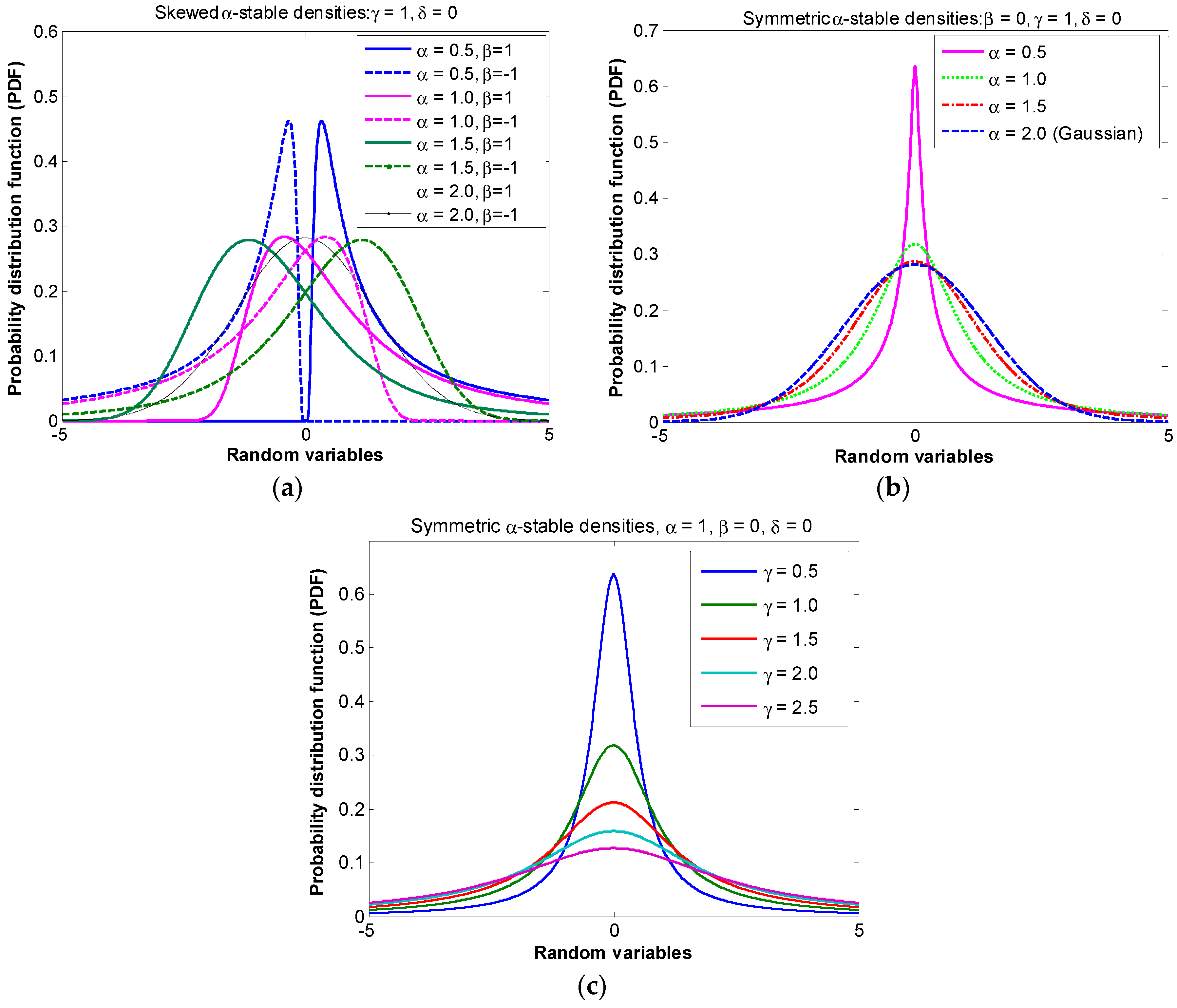
stands for the symmetrical parameter. To have a better understanding of the alpha-stable noise, its probability density function (PDF) curves are depicted in Figure 1 and Figure 2 as examples. Figure 1a shows that the PDF curve of symmetric alpha-stable noise changes with the parameter α , i.e., a smaller α produces a larger PDF of the alpha-stable noise model and vice versa. In other words, α controls the strength of the impulsive noise. Similarly, Figure 1b shows that the PDF curve of skewed α-stable noise model also changes simultaneously with α and β . Since the skewed noise model may not exist in practical wireless communication systems, the symmetrical α-stable noise model is used in this paper; the characteristic function of α-stable process reduces as
p ( t ) = exp ( γ | t | α )
For convenience, symmetric α-stable noise variance is defined by
σ z 2 = γ 2 / α
and the generalized received signal noise ratio (GSNR) is defined by
E s / N 0 ( dB ) 10 × log 10 { P 0 / γ 2 / α }
where P 0 denotes the received signal power while σ z 2 = γ 2 / α plays the same role as the noise variance.
The objective of adaptive channel estimation is to perform adaptive estimate of w ( n ) with limited complexity and memory given sequential observation { d ( n ) , x ( n ) } in the presence of additive noise z ( n ) . That is to say, the estimate observation signal y ( n ) is given as
y ( n ) = w T ( n ) x ( n )
where w ( n ) denotes channel estimator. By combining (1) and (4), the estimation error e ( n ) is
e ( n ) = d ( n ) y ( n ) = z ( n ) x T ( n ) v ( n )
where v ( n ) = w ( n ) w is the updating error of w ( n ) at iteration n . The cost function of standard LMS was written as
G L M S ( w ( n ) ) = ( 1 / 2 ) e 2 ( n )
Using Equation (11), the standard LMS algorithm was derived as
w ( n + 1 ) = w ( n ) + μ G ( w ( n ) ) w ( n ) = w ( n ) + μ e ( n ) x ( n )
where μ denotes a step-size that controls the gradient descend speed of the LMS. Letting R = E [ x ( n ) x T ( n ) ] denotes the covariance matrix of input signal x ( n ) and λ max as its maximum eigenvalue. The well-known stable convergence condition of the SLMS is
0 < μ L M S < 1 / λ max
In order to remove SαS noise, the traditional SLMS algorithm [14] was first proposed as
w ( n + 1 ) = w ( n ) + μ sgn ( e ( n ) ) x ( n )
To ensure the stability of SLMS, μ should be chosen as
0 < μ < 2 π σ e ( n ) / λ max
where σ e ( n ) denotes the unconditional variance of estimation error e ( n ) . For later theoretical analysis, the σ e 2 is conditioned by
E { e 2 ( n ) | v ( n ) } E { e 2 ( n ) } = σ e 2 ( n ) = E { [ z ( n ) v T ( n ) x ( n ) ] T [ z ( n ) v T ( n ) x ( n ) ] } = γ 2 / α + Tr { R C ( n ) }
where C ( n ) = E { v ( n ) v T ( n ) } denotes the second-order moment matrix of channel estimation error vector v ( n ) .

3. Proposed Sparse SLMS Algorithms

By incorporating sparsity-aware function into the cost function of the standard SLMS in Equation (6), sparse SLMS algorithms could be developed to take advantage of sparse structure information, to mitigate SαS noise as well as to reconstruct channel FIR. First of all, this section proposes five effective sparse SLMS algorithms with different sparse constraints. These proposed algorithms are SLMS-ZA, SLMS-RZA, SLMS-RL1, SLMS-LP, and SLMS-L0. Later, performance analysis will be given to confirm the effectiveness of the proposed algorithms.

3.1. First Proposed Algorithm: SLMS-ZA

The cost function of the LMS-ZA algorithm [7] was developed as
G Z A ( w ( n ) ) = ( 1 / 2 ) e 2 ( n ) + λ Z A w ( n ) 1
where λ Z A stands for a positive parameter to trade off instantaneous estimation square error and sparse penalty of w ( n ) . It is worth noting that the optimal selection of λ Z A is very difficult due to the fact that λ Z A depends on many variables such as channel sparsity, instantaneous updating error e ( n ) , SNR, and so on. Throughout this paper, the regularization parameter will be selected empirically via the Monte Carlo method. According to Equation (17), the LMS-ZA algorithm was developed as
w ( n + 1 ) = w ( n ) μ G Z A ( w ( n ) ) w ( n ) = w ( n ) + μ e ( n ) x ( n ) ρ Z A sgn ( w ( n ) )
where ρ Z A = μ λ Z A depends the μ and λ Z A . To mitigate the SαS noises, by constraining sign function on e ( n ) , the SLMS-ZA algorithm is developed as
w ( n + 1 ) = w ( n ) + μ sgn ( e ( n ) ) x ( n ) ρ Z A sgn ( w ( n ) )
where the first sgn ( ) function is utilized to remove impulsive noise in e ( n ) while the second one acts as a sparsity-inducing function to exploit channel sparsity in w ( n ) . Please note that the steady-state mean square error (MSE) performance of the proposed SLMS-ZA depends highly on ρ Z A .

3.2. Second Proposed Algorithm: SLMS-RZA

A stronger sparse penalty function can obtain more accurate sparse information [19]. By devising an improved sparse penalty function RZA, we can develop an improved LMS-RZA algorithm. Its cost function can be constructed as
G R Z A ( w i ( n ) ) = 1 2 e 2 ( n ) + λ R Z A i = 0 N 1 log ( 1 + ε R Z A | w i ( n ) | )
where λ R Z A > 0 is a positive parameter. By deriving Equation (20), the update equation of SLMS-RZA is obtained as
w i ( n + 1 ) = w i ( n ) + μ G R Z A ( w i ( n ) ) w i ( n ) = w i ( n ) + μ e ( n ) x ( n i ) ρ R Z A sgn ( w i ( n ) ) 1 + ε R Z A | w i ( n ) |
where ρ R Z A = μ λ R Z A ε R Z A . By collecting all of the coefficients as the matrix-vector form, Equation (21) can be expressed as
w ( n + 1 ) = w ( n ) + μ e ( n ) x ( n ) ρ R Z A sgn ( w ( n ) ) 1 + ε R Z A | w ( n ) |
where ε R Z A = 20 [7] denotes reweighted factor. By inducing sign function to constraint e ( n ) in Equation (22), the stable SLMS-RZA algorithm is proposed as
w ( n + 1 ) = w ( n ) + μ sgn ( e ( n ) ) x ( n ) ρ R Z A sgn ( w ( n ) ) 1 + ε R Z A | w ( n ) |

3.3. Third Proposed Algorithm: SLMS-RL1

In addition to the RZA in (23), RL1 function was also considered as an effective sparse constraint in the field of compressive sensing (CS) [19]. By choosing a suitable reweighted factor, δ R L 1 , RL1 could approach the optimal 0 -norm (L0) constraint. Hence, the LMS-RL1 algorithm has been considered an attractive application of sparse channel estimation. The LMS-RL1 algorithm [5] was developed as
G R L 1 ( w ( n ) ) = ( 1 / 2 ) e 2 ( n ) + λ R L 1 f ( n ) w ( n ) 1
where λ R L 1 denotes positive regularization parameter and f ( n ) is defined as
[ f ( n ) ] i = 1 δ R L 1 + | [ w ( n 1 ) ] i | ,   i = 0 , 1 , , N 1
where δ R L 1 > 0 and then [ f ( n ) ] i > 0 . By taking the derivation of Equation (24), the LMS-RL1 algorithm was updated as
w ( n + 1 ) = w ( n ) + μ G R L 1 ( w ( n ) ) w ( n ) = w ( n ) + μ e ( n ) x ( n ) ρ R L 1 sgn ( f ( n ) w ( n ) ) f T ( n ) = w ( n ) + μ e ( n ) x ( n ) ρ R L 1 sgn ( w ( n ) ) f T ( n ) = w ( n ) + μ e ( n ) x ( n ) ρ R L 1 sgn ( w ( n ) ) δ R L 1 + | w ( n 1 ) |
where ρ R L 1 = μ λ R L 1 . The third step of derivation can be obtained since sgn ( f ( n ) ) = 1 1 × N and then sgn ( f ( n ) w ( n ) ) = sgn ( w ( n ) ) . Here the cost function G R L 1 ( n ) is convex due to the fact that it does not depend on w ( n ) . Likewise, sign function is adopted for constraint e ( n ) and then robust SLMS-RL1 algorithm is obtained as
w ( n + 1 ) = w ( n ) + μ sgn ( e ( n ) ) x ( n ) ρ R L 1 sgn ( w ( n ) ) δ R L 1 + | w ( n 1 ) |

3.4. Fourth Proposed Algorithm: SLMS-LP

p -norm sparse penalty is a nonconvex function to exploit sparse prior information. In [5], LMS-LP based channel estimation algorithms was developed as
G L P ( w ( n ) ) = ( 1 / 2 ) e 2 ( n ) + λ L P w ( n ) p
where λ L P > 0 is a positive parameter. The update function of LMS-LP is given as
w ( n + 1 ) = w ( n ) μ G L P ( w ( n ) ) w ( n ) = w ( n ) + μ e ( n ) x ( n ) ρ L P w ( n ) p 1 p sgn ( w ( n ) ) ε L P + | w ( n ) | 1 p
where ε L P > 0 is a threshold parameter and ρ L P = μ λ L P . To remove the SαS noise, SLMS-LP based robust adaptive channel estimation is written as
w ( n + 1 ) = w ( n ) + μ sgn ( e ( n ) ) x ( n ) ρ L P w ( n ) p 1 p sgn ( w ( n ) ) ε L P + | w ( n ) | 1 p

3.5. Fifth Proposed Algorithm: SLMS-L0

It is well known that the 0 -norm penalty can exploit the sparse structure information. Hence, the L0-LMS algorithm is constructed as
G L 0 ( w ( n ) ) = 1 2 e 2 ( n ) + λ L 0 w ( n ) 0
where λ L 0 > 0 and w ( n ) 0 stands for optimal 0 -norm function. However, it is a NP-hard problem to solve the 0 -norm sparse minimization [22]. The NP-hard problem in Equation (31) can be solved by an approximate continuous function:
w ( n ) 0 i = 0 N 1 ( 1 e θ | w i ( n ) | )
Then, the previous cost function (29) is changed to
G L 0 ( w ( n ) ) = 1 2 e 2 ( n ) + λ L 0 i = 0 N 1 ( 1 e θ | w i ( n ) | )
The first-order Taylor series expansion of exponential function e θ | w i ( n ) | can be expressed as
e θ | w i ( n ) | { 1 θ | w i ( n ) | , w h e n   | w i ( n ) | 1 / θ 0 , o t h e r s
Then, the LMS-L0 based robust adaptive sparse channel estimation algorithm is given as
w ( n + 1 ) = w ( n ) + μ e ( n ) x ( n ) ρ L 0 sgn ( w ( n ) ) e θ | w ( n ) |
where ρ L 0 = μ λ L 0 . In Equation (35), the exponential function still exhausts high computational resources. To further reduce it, a simple approximation function ζ ( w ( n ) ) is proposed in [20]. By introducing sign function into Equation (35), the SLMS-L0 based robust channel estimation algorithm is written as
w ( n + 1 ) = w ( n ) + μ sgn ( e ( n ) ) x ( n ) ρ L 0 ζ ( w ( n ) )
where ρ L 0 = μ λ L 0 and ζ ( w i ( n ) ) are defined as
ζ ( w i ( n ) ) = { 2 θ 2 w i ( n ) 2 θ sgn ( w i ( n ) ) , w h e n | w i ( n ) | 1 / θ 0 , o t h e r s
for ζ ( w ( n ) ) = [ ζ ( w 0 ( n ) ) , ζ ( w 1 ( n ) ) , , ζ ( w N 1 ( n ) ) ] T .

4. Convergence Analysis of the Proposed Algorithms

Unlike the standard SLMS algorithm, the proposed sparse SLMS algorithms can further improve estimation accuracy by exploiting channel sparsity. For convenience of theoretical analysis without loss of generality, the above proposed sparse SLMS algorithms are generalized as
w ( n + 1 ) = w ( n ) + μ sgn ( e ( n ) ) x ( n ) ρ f ( w ( n ) )
where f ( w ( n ) ) denotes sparsity constraint function and ρ denotes the regularization parameter. Throughout this paper, our analysis is based on independent assumptions as below:
E ( z ( n ) x ( n ) ) = 0
E [ z ( n ) x ( n ) v T ( n ) ] = 0
E [ z ( n ) v ( n ) x T ( n ) ] = 0
E [ z ( n ) f ( w ( n ) ) x T ( n ) ] = 0
E [ z ( n ) x ( n ) f T ( w ( n ) ) ] = 0
Theorem 1. 
If μ satisfies (15), the mean coefficient vector E { w ( n ) } approaches
w ( ) = w π / 2 μ 1 ρ R 1 γ 1 / α f ( w ( ) )
Proof. 
By subtracting w from both sides of (35), the mean estimation error E { v ( n + 1 ) } is derived as
E { v ( n + 1 ) } = E { v ( n ) } + μ E { sgn ( e ( n ) ) x ( n ) } ρ f ( w ( n ) ) E { v ( n ) } + μ E { sgn ( e ( n ) ) x ( n ) | v ( n ) } ρ f ( w ( n ) ) = E { v ( n ) } + 2 / π μ σ e 1 ( n ) E { e ( n ) x ( n ) } ρ f ( w ( n ) ) = { I 2 / π μ σ e 1 ( n ) R } E { v ( n ) } ρ f ( w ( n ) )
It is worth mentioning that vector ρ f ( w ( n ) ) is bounded for all sparse constraints. For example, if f ( w ( n ) ) = sgn ( w ( n ) ) , then the bound is between ρ I N and ρ I N , where I N is an N -length identity vector. For n , Equation (45) can be rewritten as
E { v ( ) } = { I 2 / π μ σ e 1 ( ) R } E { v ( ) } ρ f ( w ( ) ) { I 2 / π μ γ 1 / α R } E { v ( ) } ρ f ( w ( ) )
where Tr ( R C ( ) ) = σ x 2 c ( ) γ 1 / α and
σ e 2 ( ) = lim n σ e 2 ( n ) = γ 2 / α + Tr ( R C ( ) ) γ 2 / α
are utilized in the above equation. Since E { w ( ) } = w E { v ( ) } , according to Equation (47), one can easily get Theorem 1.
Theorem 2. 
Let Ω denotes the index set of nonzero taps, i.e., w i 0 for i Ω . Assuming ρ is sufficiently small so that for every i Ω , the excess MSE of sparse SLMS algorithms is
P e x ( ) = μ γ 1 / α φ 2 2 π φ 1 + ρ γ 1 / α η 1 2 π μ φ 1 ( ρ η 2 η 1 )
where φ 1 , φ 2 , η 1 and η 2 are defined as:
φ 1 = Tr [ ( I 2 / π μ σ e 1 R ) 1 ]
φ 2 = Tr [ R ( I 2 / π μ σ e 1 R ) 1 ]
η 1 N 1 2 / π μ γ 1 / α λ max
η 2 2 E { Tr [ w ( ) f T ( w ( ) ) ] } 2 E { Tr [ w f T ( w ( ) ) ] }
Proof. 
By using the above independent assumptions in Equations (49)–(52), the second moment C ( n + 1 ) of the weight error vector v ( n + 1 ) can be evaluated recursively as
C ( n + 1 ) = E { v ( n + 1 ) v T ( n + 1 ) } = E { [ v ( n ) + μ sgn ( e ( n ) ) x ( n ) ρ f ( w ( n ) ) ] [ v ( n ) + μ sgn ( e ( n ) ) x ( n ) ρ f ( w ( n ) ) ] T } = E { v ( n ) v T ( n ) } + μ 2 E { x ( n ) x T ( n ) } + μ { E [ sgn ( e ( n ) ) v ( n ) x T ( n ) ] + E [ sgn ( e ( n ) ) x ( n ) v T ( n ) ] } A 1 ( n ) μ ρ { E [ sgn ( e ( n ) ) x ( n ) f T ( w ( n ) ) ] + E [ sgn ( e ( n ) ) f ( w ( n ) ) x T ( n ) ] } A 2 ( n ) ρ { E [ v ( n ) f T ( w ( n ) ) ] + E [ f ( w ( n ) ) v T ( n ) ] } A 3 ( n ) + ρ 2 E { f ( w ( n ) ) f T ( w ( n ) ) } A 4 ( n ) = C ( n ) + μ 2 R + A 1 ( n ) ( A 2 ( n ) + A 3 ( n ) ) A 5 ( n ) + A 4 ( n )
where A 1 ( n ) , A 2 ( n ) , and A 5 ( n ) are further derived as
A 1 ( n ) μ E { sgn ( e ( n ) ) v ( n ) x T ( n ) | v ( n ) } + μ E { sgn ( e ( n ) ) x ( n ) v T ( n ) | v ( n ) } = π / 2 μ σ e 1 ( n ) { E [ v ( n ) E [ e ( n ) x T ( n ) | v ( n ) ] ] + E [ E [ e ( n ) x ( n ) | v ( n ) ] v T ( n ) ] } = π / 2 μ σ e 1 ( n ) { E [ v ( n ) v T ( n ) ] R + R E [ v ( n ) v T ( n ) ] } = π / 2 μ σ e 1 ( n ) [ C ( n ) R + R C ( n ) ]
A 2 ( n ) = μ ρ { E [ sgn ( e ( n ) ) x ( n ) f T ( w ( n ) ) ] + E [ sgn ( e ( n ) ) f ( w ( n ) ) x T ( n ) ] } μ ρ E { E [ sgn ( e ( n ) ) x ( n ) f T ( w ( n ) ) | v ( n ) ] + E [ sgn ( e ( n ) ) f ( w ( n ) ) x T ( n ) | v ( n ) ] } = 2 / π μ ρ σ e 1 E { E [ x ( n ) e ( n ) | v ( n ) ] f T ( w ( n ) ) + f ( w ( n ) ) E [ e ( n ) x T ( n ) | v ( n ) ] } = 2 / π μ ρ σ e 1 { R E [ v ( n ) f T ( w ( n ) ) ] + E [ f ( w ( n ) ) v T ( n ) ] R }
A 5 ( n ) A 2 ( n ) + A 3 ( n ) = 2 / π μ ρ σ e 1 { R E [ v ( n ) f T ( w ( n ) ) ] + E [ f ( w ( n ) ) v T ( n ) ] R } + ρ { E [ v ( n ) f T ( w ( n ) ) ] + E [ f ( w ( n ) ) v T ( n ) ] } = ρ ( I 2 / π μ σ e 1 R ) E [ v ( n ) f T ( w ( n ) ) ] + ρ E [ f ( w ( n ) ) v T ( n ) ] ( I 2 / π μ σ e 1 R )
By substituting Equations (54) and (56) into Equation (53), we obtain
C ( n + 1 ) = C ( n ) + μ 2 R + A 1 ( n ) A 5 ( n ) + A 4 ( n ) = C ( n ) + μ 2 R 2 / π μ σ e 1 ( n ) [ C ( n ) R + R C ( n ) ] A 5 ( n ) + A 4 ( n )
Letting n and using Equation (47), Equation (57) is further rewritten as
C ( ) R + R C ( ) 2 / π μ γ 1 / α R + 2 / π μ 1 γ 1 / α lim n [ A 4 ( n ) A 5 ( n ) ]
Multiplying both sides of Equation (58) by ( I 2 / π μ σ e 1 R ) 1 from right, the following can be derived as
[ C ( ) R + R C ( ) ] ( I 2 / π μ σ e 1 R ) 1 2 / π μ γ 1 / α R ( I 2 / π μ σ e 1 R ) 1 + 2 / π μ 1 γ 1 / α lim n A 4 ( n ) ( I 2 / π μ σ e 1 R ) 1 n 2 / π μ 1 γ 1 / α lim n A 5 ( n ) ( I 2 / π μ σ e 1 R ) 1
Taking the trace of the two sides of Equation (59), since Tr ( C ( ) R ) = Tr ( R C ( ) ) , the excess MSE is derived as
P e x ( ) = Tr [ R C ( ) ] = 2 / π μ γ 1 / α 2 φ 1 Tr [ R ( I 2 / π μ σ e 1 R ) 1 ] φ 2 + 2 / π μ 1 γ 1 / α 2 φ 1 lim n Tr [ A 4 ( n ) ( I 2 / π μ σ e 1 R ) 1 ] η 1 ( n ) 2 / π μ 1 γ 1 / α 2 φ 1 lim n Tr [ A 5 ( n ) ( I 2 / π μ σ e 1 R ) 1 ] η 2 ( n )
The matrix ( I 2 / π μ γ 1 / α R ) is symmetric, and its eigenvalue decomposition can be written as
I 2 / π μ γ 1 / α R = U V U T
with U being the orthonormal matrix of eigenvectors and V being a diagonal matrix of eigenvalues. Therefore, ( I 2 / π μ σ e 1 R ) = U V 1 U T . Let λ max be the largest eigenvalue of the covariance matrix R and μ be small enough such that ( 1 2 / π μ γ 1 / α λ max ) 1 > 0 under certain noise cases. Since V 1 is a diagonal matrix, elements are all non-negative and less than or equal to ( 1 2 / π μ γ 1 / α λ max ) 1 , hence, η 1 lim n   η 1 ( n ) and η 2 lim n   η 2 ( n ) are further derived as
η 1 lim n η ( n ) = lim n Tr { A 4 ( I 2 / π μ σ e 1 R ) 1 } = lim n ρ 2 E { Tr [ f ( w ( n ) ) ( I 2 / π μ γ 1 / α R ) 1 f T ( w ( n ) ) ] } = lim n ρ 2 E { Tr [ f ( w ( n ) ) U V 1 U T f T ( w ( n ) ) ] } = lim n ρ 2 E { Tr [ V 1 U T f ( w ( n ) ) f T ( w ( n ) ) U ] } lim n ρ 2 1 2 / π μ γ 1 / α λ max E { Tr [ U T f ( w ( n ) ) f T ( w ( n ) ) U ] } = ρ 2 1 2 / π μ γ 1 / α λ max E { Tr [ f T ( w ( ) ) U U T f ( w ( ) ) ] } ρ 2 1 2 / π μ γ 1 / α λ max E { f T ( w ( ) ) f ( w ( ) ) } N ρ 2 1 2 / π μ γ 1 / α λ max
η 2 lim n η 2 ( n ) = lim n Tr { A 5 ( I 2 / π μ σ e 1 R ) 1 } = lim n ρ E { Tr [ v ( n ) f T ( w ( n ) ) + f ( w ( n ) ) v T ( n ) ] } = lim n 2 ρ E { Tr [ v ( n ) f T ( w ( n ) ) ] } = lim n 2 ρ E { Tr [ w ( n ) f T ( w ( n ) ) ] } 2 ρ E { Tr [ w f T ( w ( n ) ) ] } = 2 ρ E { Tr [ w ( ) f T ( w ( ) ) ] } 2 ρ E { Tr [ w f T ( w ( ) ) ] } .
Substituting Equations (62) and (63) into Equation (60), the excess MSE is finally derived as
P e x ( ) = μ γ 1 / α φ 2 2 π φ 1 + ρ γ 1 / α η 1 2 π μ φ 1 ( ρ η 2 η 1 )
where η 1 η 1 / ρ 2 and η 2 η 2 / ρ 2 . According to Equation (62), one can find that η 1 is bound as
0 < η 2 N 1 2 / π μ γ 1 / α λ max
The excess MSE of sparse SLMS in Equation (65) implies that choosing suitable ρ < η 1 / η 2 can lead to smaller excess MSE than standard SLMS algorithm.

5. Numerical Simulations and Discussion

To evaluate the proposed robust channel estimation algorithms, we compare these algorithms in terms of channel sparsity and non-Gaussian noise level. A typical broadband wireless communication system is considered in computer simulations [3]. The baseband bandwidth is assigned as 60 MHz and the carrier frequency is set as 2.1 GHz. Signal multipath transmission causes the 1.06   μ s delay spread. According to the Shannon sampling theory, the channel length is equivalent to n = 128. In addition, average mean square error (MSE) is adopted for evaluate the estimation error. The MSE is defined as
MSE { w ( n ) } ( dB ) 10 log 10 ( 1 / M ) m = 1 M w ( n ) w 2 2 / w 2 2 ,
where w and denote actual channel and estimator, respectively. M = 1000 independent runs are adopted for Monte Carlo simulations. The nonzero channel taps are generated to satisfy random Gaussian distribution as C N ( 0 , σ w 2 I ) and all of these positions are randomly allocated within w , which is normalized as E { w 2 2 } = 1 . All of the simulation parameters are listed in Table 1.

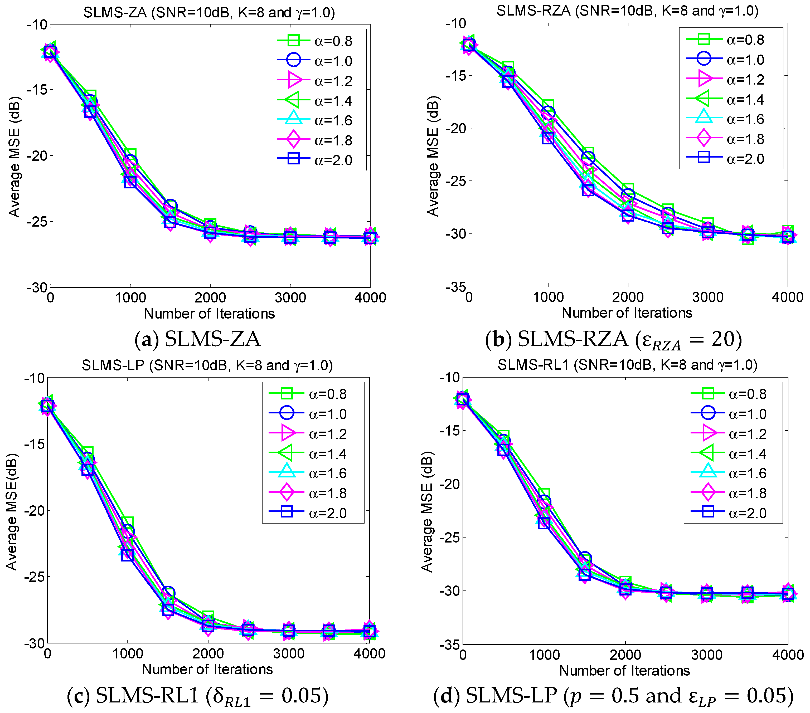
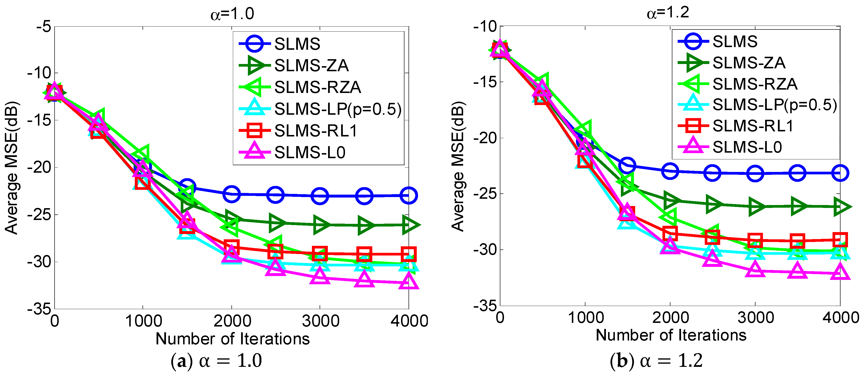
5.1. Experiment 1. MSE Curves of Proposed Algorithms vs. Different Alpha-Stable Noise

The proposed robust adaptive sparse channel estimation algorithms are evaluated with respect to α in the scenarios of K = 8 and SNR = 10 dB, as shown in Figure 2. Under different alpha-stable noise regimes, i.e., α { 1.0 , 1.2 , 1.4 , 1.6 , 1.8 } , our proposed algorithms can achieve much better MSE performance than standard SLMS. With different sparsity constraint functions, i.e., ZA, RZA, LP, RL1, and L0, different performance gain could be obtained. Since L0-norm constraint exploits channel sparsity most efficiently in these sparse constraint functions, Figure 2 shows that the lowest MSE of SLMS-L0 results in the lowest MSE. Indeed, Figure 2 implies that taking more channel sparse structure information can obtain more performance gain. Hence, selecting an efficient sparse constraint function is an important step in devising sparse SLMS algorithms. In addition, it is worth noting that the convergence speed of SLMS-RZA is slightly slower than other sparse SLMS algorithms while its steady-state MSE performance as good as SLMS-LP. According to Figure 2, proposed SLMS algorithms are confirmed by simulation results in different impulsive noise cases.

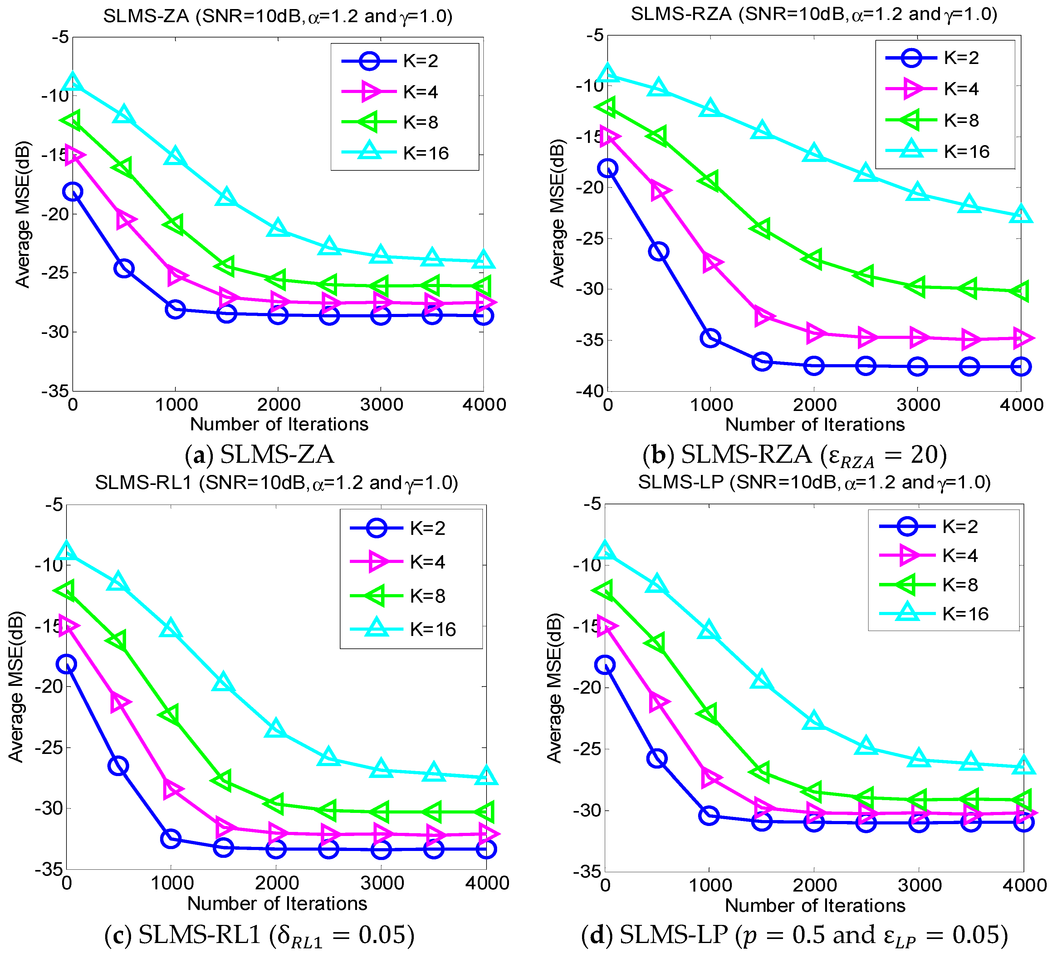
5.2. Experiment 2. MSE Curves of Proposed Algorithms vs. Channel Sparsity

Our proposed channel estimation algorithms are evaluated with channel sparsity K { 2 ,   4 ,   8 ,   16 } in the scenarios of α = 1.2 , γ = 1.0 , K = 8 and S N R = 10   dB , as shown in Figure 3. We can find that the proposed sparse SLMS algorithms depend on channel sparsity K , i.e., our proposed algorithms obtained correspondingly better MSE performance in a scenario of sparser channels. In other words, exploiting more channel sparsity information could produce more performance gain and vice versa. Hence, the proposed methods are effective to exploit channel sparsity as well as remove non-Gaussian α-stable noise.

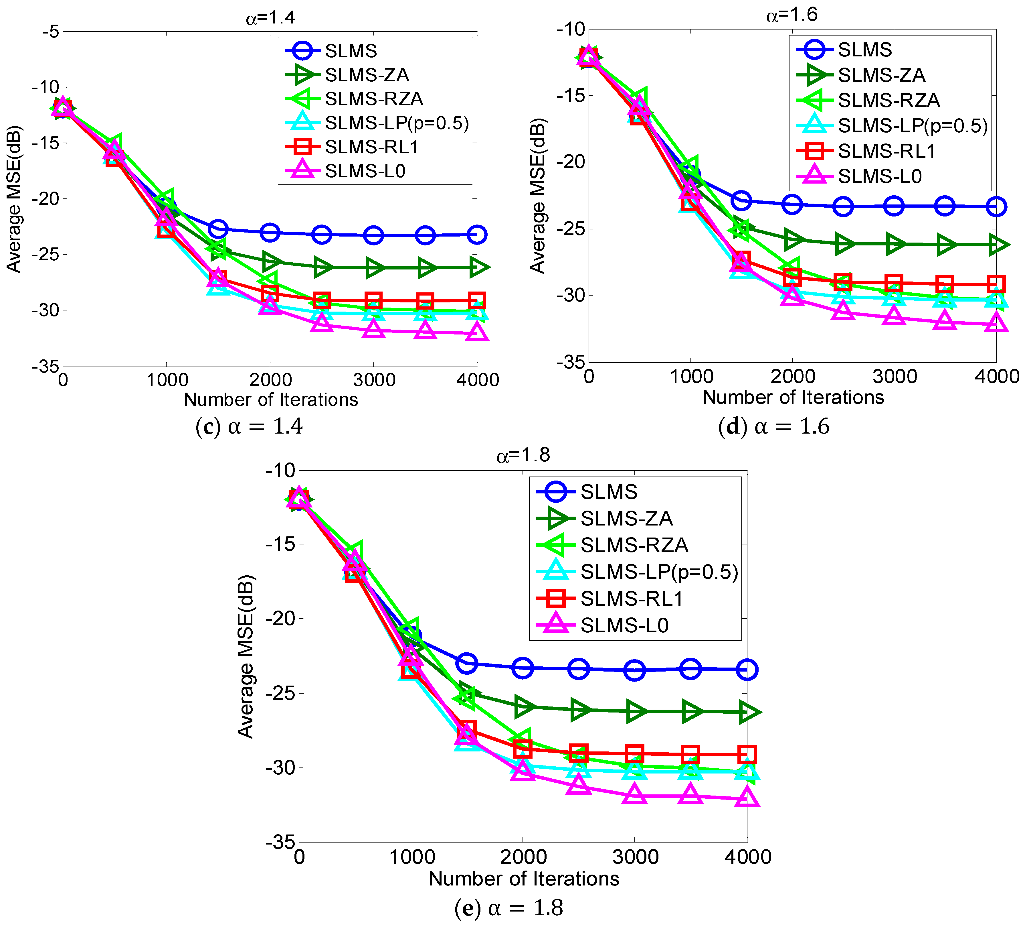
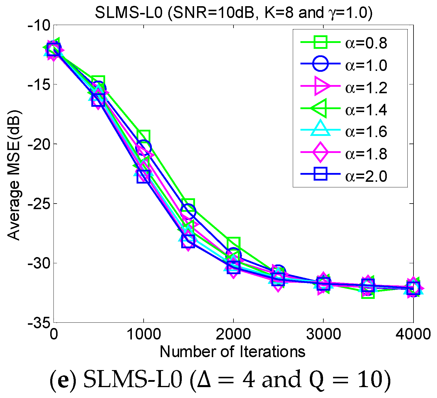
5.3. Experiment 3. MSE Curves of Proposed Algorithms vs. Characteristic Exponent

The average MSE curves of the proposed algorithm with respect to characteristic exponent α { 0.8 ,   1.0 ,   1.2 ,   1.4 ,   1.6 ,   1.8 ,   2.0 } in scenarios of dispersion parameter γ = 1.0 , channel length N = 128 , channel sparsity K = 8 and S N R = 10   dB , are depicted as shown in Figure 4. The proposed algorithm is very stable for the different strengths of impulsive noises that are controlled by the characteristic exponent α . In addition, it is very interesting that the convergence speed of the proposed SLMS algorithms may be reduced by the relatively small α . The main reason the proposed SLMS algorithm is utilized is that the sign function is stable at different values of α . Hence, the proposed algorithm can mitigate non-Gaussian α-stable noise.

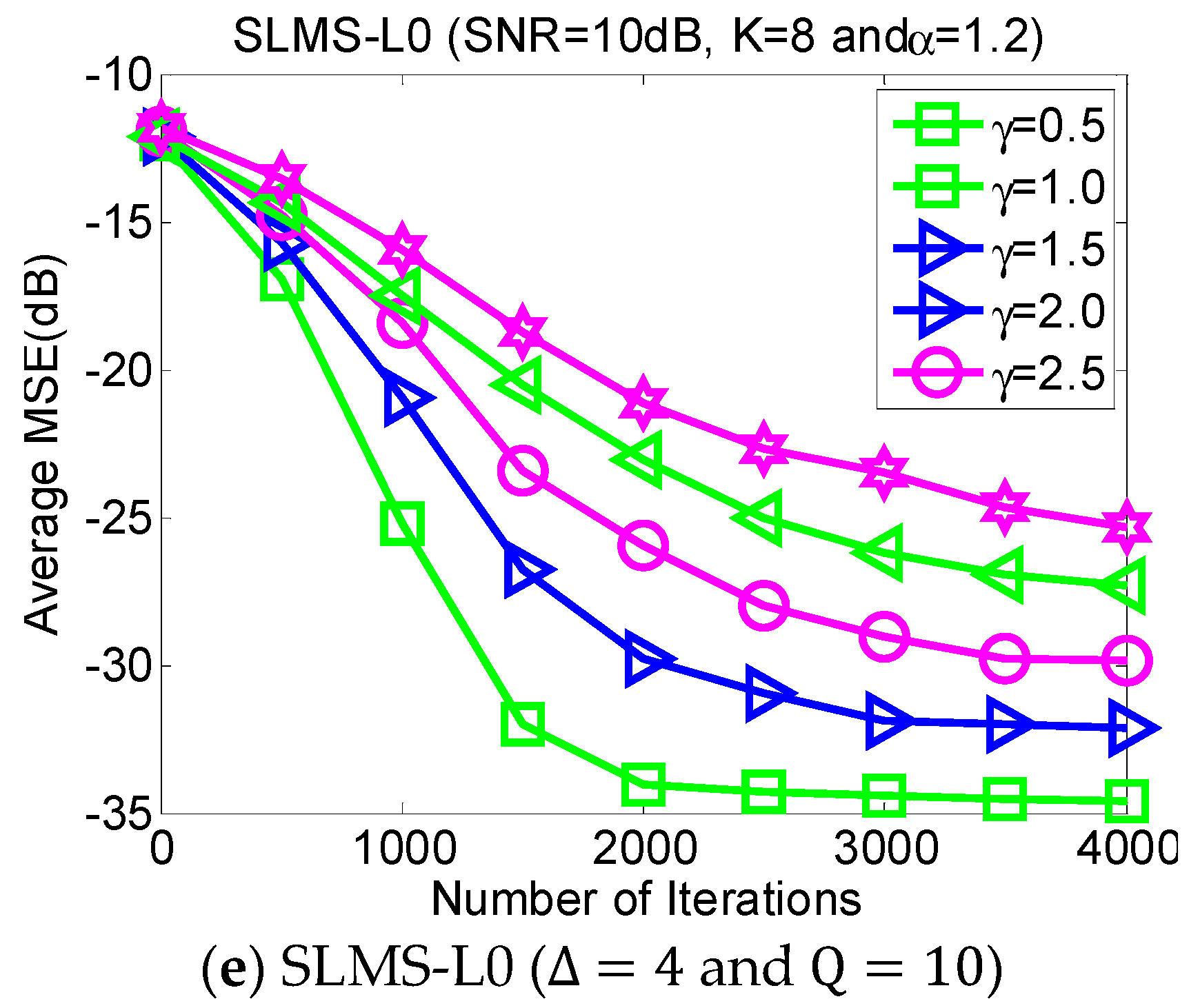
5.4. Experiment 4. MSE Curves of Proposed Algorithms vs. Dispersive Parameter

Dispersive distribution of α -stable noise has harmful effects. This experiment evaluates the MSE performance of proposed SLMS algorithms in different dispersive parameters γ { 0.5 ,   1.0 ,   1.5 ,   2.0 ,   2.5 } in the scenarios of α = 1.2 , K = 8 , and SNR = 10 dB, as shown in Figure 5. Larger γ means more serious dispersion of α-stable noise and a worse performance for the proposed algorithm and vice versa. Figure 5 implies that the proposed SLMS algorithms are deteriorated by γ rather than α . The main reason is that the proposed SLMS algorithm can mitigate the amplitude effect of the α -stable noise due to the fact that the sign function is utilized in the proposed SLMS algorithms.

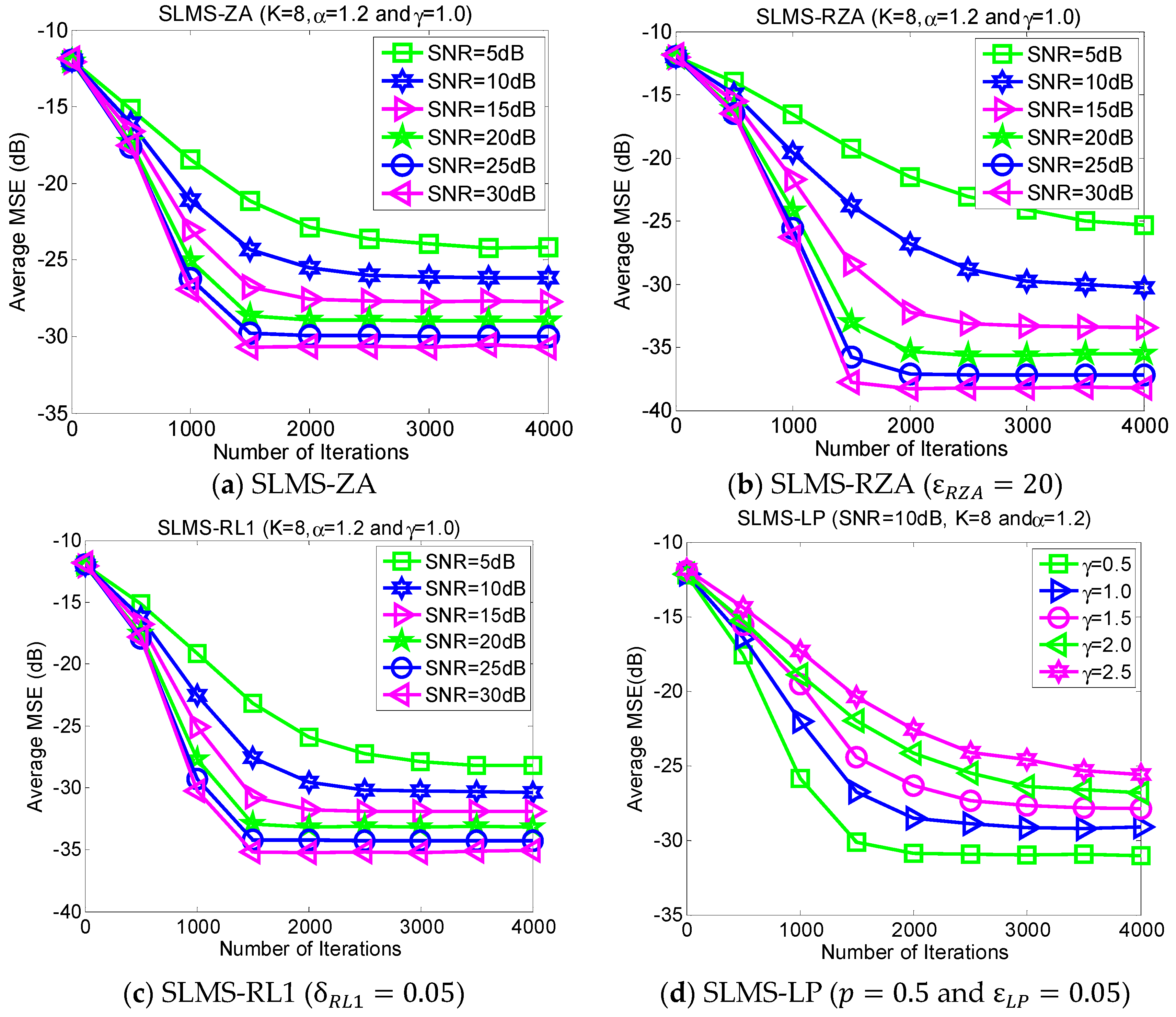
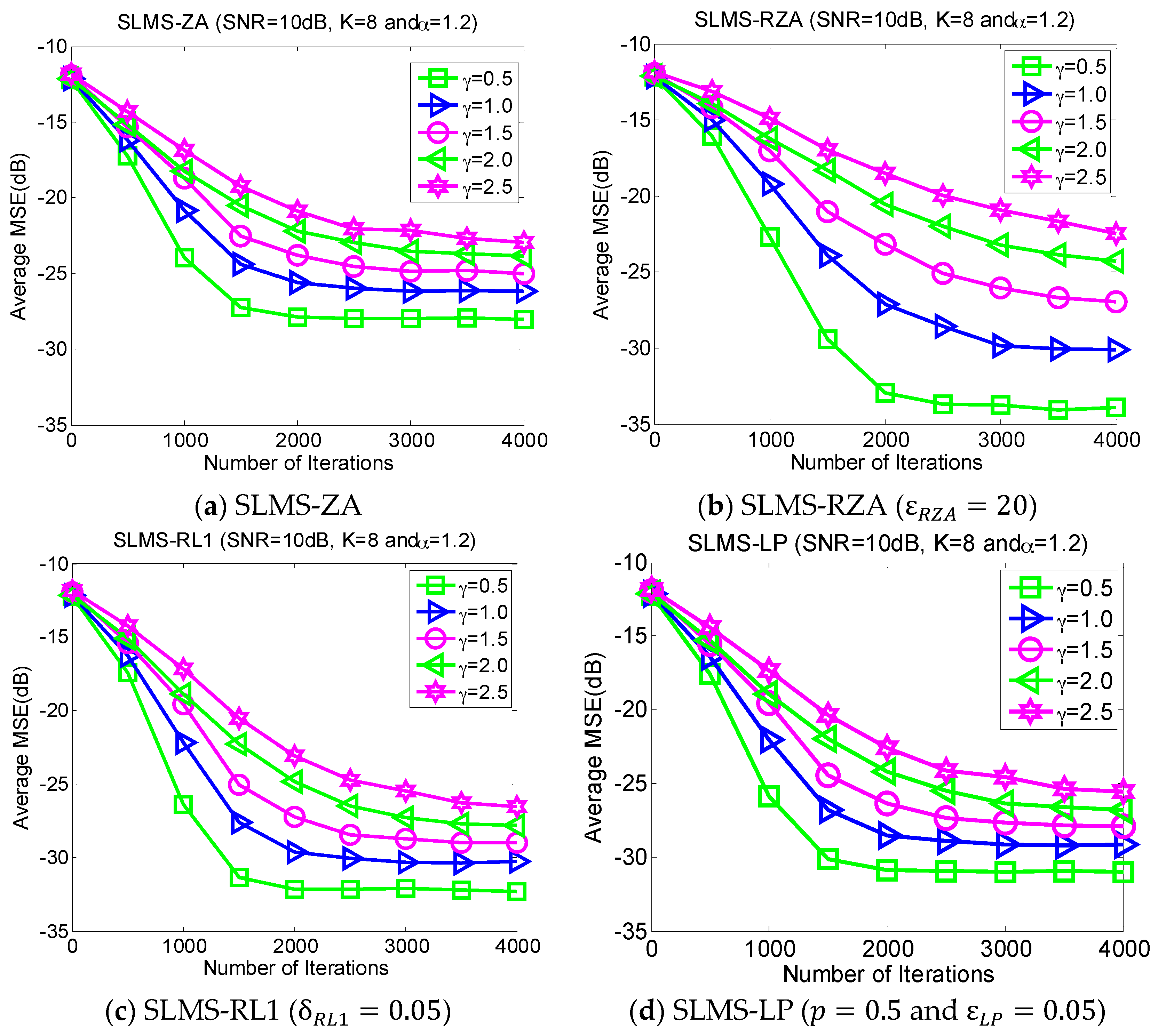
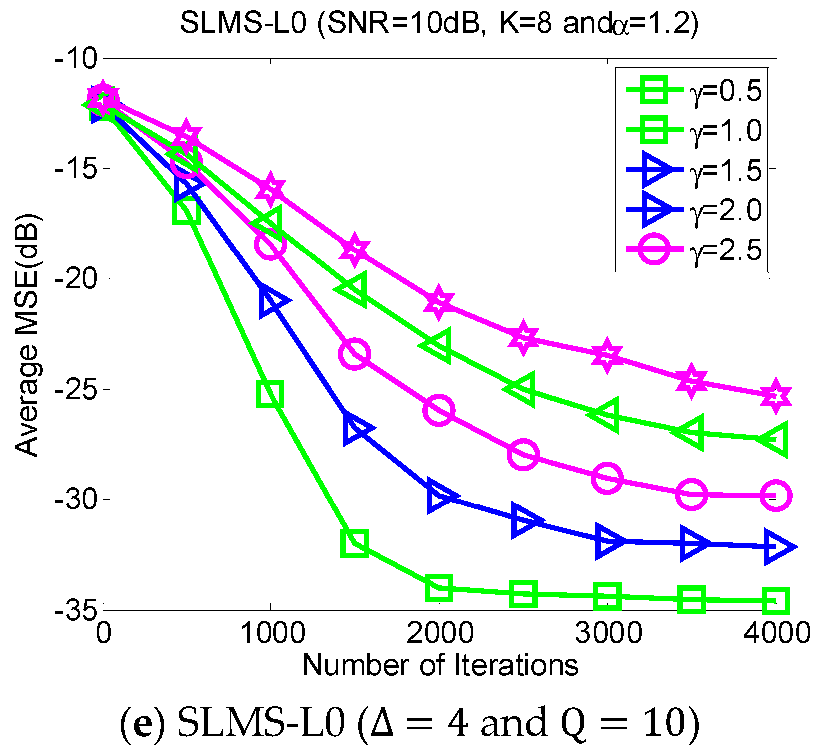
5.5. Experiment 5. MSE Curves of Proposed Algorithms vs. SNR

In the different SNR regimes, the average MSE curves of the proposed algorithms are demonstrated in Figure 6 in the scenarios of characteristic exponent α = 1.2 , dispersive parameter γ = 1.0 , channel length N = 128 , and channel sparsity K = 8 . The purpose of directing figures in Figure 6 is to further confirm the effectiveness of the proposed algorithms under different SNR regimes.

6. Conclusions

Based on SαS noise model, we have proposed five sparse SLMS algorithms for robust channel estimation in this paper by introducing sparsity-inducing penalty functions into the standard SLMS algorithm so that channel sparsity can be exploited to improve the channel estimation performance. Theoretical analysis verified the convergence of the proposed algorithms in terms of mean and excess MSE. Numerical simulations were provided to validate the performance gain of our proposed algorithm.

Acknowledgments

The authors would like to express their appreciation to the anonymous reviewers for their constructive comments and positive suggestions. This work was supported by a National Natural Science Foundation of China grant (61271240), the Scientific and Technological Research Program of Chongqing Municipal Education Commission (KJ1500515), and the project of the Fundamental and Frontier Research plan of Chongqing (cstc2016jcycA0022).

Author Contributions

Tingping Zhang derived the sparse channel estimation algorithms and wrote the paper; Guan Gui and Tingping Zhang performed the experiments; Tingping Zhang wrote the paper; and Guan Gui checked the paper.

Conflicts of Interest

The authors declare no conflict of interest.

References

  1. Adachi, F.; Garg, D.; Takaoka, S.; Takeda, K. Broadband CDMA techniques. IEEE Wirel. Commun. 2005, 12, 8–18. [Google Scholar] [CrossRef]
  2. Raychaudhuri, B.D.; Mandayam, N.B. Frontiers of wireless and mobile communications. Proc. IEEE 2012, 100, 824–840. [Google Scholar] [CrossRef]
  3. Dai, L.; Wang, Z.; Yang, Z. Next-generation digital television terrestrial broadcasting systems: Key technologies and research trends. IEEE Commun. Mag. 2012, 50, 150–158. [Google Scholar] [CrossRef]
  4. Haykin, S. Adaptive Filter Theory; Prentice-Hall: Englewood Cliffs (Upper Saddle River), NJ, USA, 1996. [Google Scholar]
  5. Taheri, O.; Vorobyov, S.A. Sparse channel estimation with Lp-norm and reweighted L1-norm penalized least mean squares. In Proceedings of the 2011 IEEE International Conference on Acoustics, Speech and Signal Processing (ICASSP), Prague, Czech Republic, 22–27 May 2011; pp. 2864–2867.
  6. Gui, G.; Peng, W.; Adachi, F. Improved adaptive sparse channel estimation based on the least mean square algorithm. In Proceedings of the 2013 IEEE Wireless Communications and Networking Conference (WCNC), Shanghai, China, 7–10 April 2013; pp. 3105–3109.
  7. Chen, Y.; Gu, Y.; Hero, A.O., III. Sparse LMS for system identification. In Proceedings of the 2009 IEEE International Conference on Acoustics, Speech and Signal Processing, Taipei, Taiwan, 19–24 April 2009; pp. 3125–3128.
  8. Chen, B.; Zhao, S.; Zhu, P.; Principe, J.C. Quantized kernel least mean square algorithm. IEEE Trans. Neural Netw. Learn. Syst. 2012, 23, 22–32. [Google Scholar] [CrossRef] [PubMed]
  9. Li, Y.; Hamamura, M. Zero-attracting variable-step-size least mean square algorithms for adaptive sparse channel estimation. Int. J. Adapt. Control Signal Process. 2015. [Google Scholar] [CrossRef]
  10. Li, Y.; Li, W.; Yu, W.; Wan, J.; Li, Z. Sparse adaptive channel estimation based on lp-norm-penalized affine projection algorithm. Int. J. Antennas Propag. 2014. [Google Scholar] [CrossRef]
  11. Lin, J.; Member, S.; Nassar, M.; Evans, B.L. Impulsive noise mitigation in powerline communications using sparse Bayesian learning. IEEE J. Sel. Areas Commun. 2013, 31, 1172–1183. [Google Scholar] [CrossRef]
  12. Shao, M.; Nikias, C.L. Signal processing with fractional lower order moments: Stable processes and their applications. Proc. IEEE 1993, 81, 986–1010. [Google Scholar] [CrossRef]
  13. Middleton, D. Non-Gaussian noise models in signal processing for telecommunications: New methods and results for Class A and Class B noise models. IEEE Trans. Inf. Theory 1999, 45, 1129–1149. [Google Scholar] [CrossRef]
  14. Li, Y.-P.; Lee, T.-S.; Wu, B.-F. A variable step-size sign algorithm for channel estimation. Signal Process. 2014, 102, 304–312. [Google Scholar] [CrossRef]
  15. Shao, T.; Zheng, Y.; Benesty, J. An affine projection sign algorithm robust against impulsive interferences. IEEE Signal Process. Lett. 2012, 17, 327–330. [Google Scholar] [CrossRef]
  16. Yoo, J.; Shin, J.; Park, P. Variable step-size affine projection aign algorithm. IEEE Trans. Circuits Syst. Express Briefs 2014, 61, 274–278. [Google Scholar]
  17. Dai, L.; Gui, G.; Wang, Z.; Yang, Z.; Adachi, F. Reliable and energy-efficient OFDM based on structured compressive sensing. In Proceedings of the IEEE International Conference on Communications (ICC), Sydney, Australia, 10–14 June 2014; pp. 1–6.
  18. Gui, G.; Peng, W.; Adachi, F. Sub-nyquist rate ADC sampling-based compressive channel estimation. Wirel. Commun. Mob. Comput. 2015, 15, 639–648. [Google Scholar] [CrossRef]
  19. Candes, E.J.; Wakin, M.B.; Boyd, S.P. Enhancing sparsity by reweighted L1 minimization. J. Fourier Anal. Appl. 2008, 14, 877–905. [Google Scholar] [CrossRef]
  20. Gu, Y.; Jin, J.; Mei, S. L0-norm constraint LMS algorithm for sparse system identification. IEEE Signal Process. Lett. 2009, 16, 774–777. [Google Scholar]
  21. Gui, G.; Xu, L.; Ma, W.; Chen, B. Robust adaptive sparse channel estimation in the presence of impulsive noises. In Proceedings of the IEEE International Conference on Digital Signal Processing (DSP), Singpore, 21–24 July 2015; pp. 1–5.
  22. Donoho, D.L.; Huo, X. Uncertainty principles and ideal atomic decomposition. IEEE Trans. Inf. Theory 2001, 47, 2845–2862. [Google Scholar] [CrossRef]
Figure 1. PDF comparisons of α-stable noise: (a) symmetric distribution; (b) skewed distribution; (c) scale distribution.
Algorithms 09 00054 g001
Figure 2. Monte Carlo based MSE curves averaging over 1000 runs with respect to different characteristic exponents α { 1.0 ,   1.2 ,   1.4 ,   1.6 ,   1.8 } , in scenarios of dispersion parameter γ = 1.0 , channel sparsity K = 8 , channel length N = 128 , and S N R = 10  dB .
Algorithms 09 00054 g002aAlgorithms 09 00054 g002b
Figure 3. Monte Carlo based MSE curves averaging over 1000 runs with respect to different channel sparsities K { 2 ,   4 ,   8 ,   16 } , in scenarios of characteristic exponent α = 1.2 , dispersion parameter γ = 1.0 , channl length N = 128 , and S N R = 10   dB .
Algorithms 09 00054 g003aAlgorithms 09 00054 g003b
Figure 4. Monte Carlo based MSE curves averaging over 1000 runs with respect to different characteristic exponents α { 0.8 ,   1.0 ,   1.2 ,   1.4 ,   1.6 ,   1.8 ,   2.0 } , in scenarios of dispersion parameter γ = 1.0 , channel length N = 128 , channel sparsity K = 8 , and S N R = 10   dB .
Algorithms 09 00054 g004aAlgorithms 09 00054 g004b
Figure 5. Monte Carlo based MSE curves averaging over 1000 runs with respect to different dispersion parameters γ { 0.5 , 1.0 , 1.5 ,   2.0 ,   2.5 } , in scenarios of characteristic exponent α = 1.2 , channel length N = 128 , channel sparsity K = 8 , and S N R = 10   dB .
Algorithms 09 00054 g005aAlgorithms 09 00054 g005b
Figure 6. Monte Carlo based MSE curves averaging over 1000 runs with respect to different SNR regimes S N R { 5   dB ,   10   dB ,   15   dB , 20   dB , 25   dB , 30   dB } in scenarios of characteristic exponent α = 1.2 , dispersive parameter γ = 1.0 , channel length N = 128 , and channel sparsity K = 8 .
Algorithms 09 00054 g006aAlgorithms 09 00054 g006b
Table 1. List of computer simulation parameters in robust adaptive sparse channel estimation.
ParametersValues
Training sequencePseudo-random binary sequence
Non-Gaussian noise level α { 1.0 , 1.2 , 1.4 , , 1.6 , 1.8 , 2.0 } , β = 0 ,   γ { 0.5 ,   1.0 ,   1.5 ,   2.0 ,   2.5 } , δ = 0
Channel length N = 128
No. of nonzero coefficients K { 2 , 4 , 8 , 16 }
Distribution of nonzero coefficientRandom Gaussian C N ( 0 , 1 )
Received SNR 5   dB ~ 30   dB
Gradient descend step size μ = 0.005
Sparsity-aware positive parameters (i.e., ρ Z A = μ λ Z A ) ρ Z A = 2 × 10 4 , ρ R Z A = 2 × 10 3
ρ R L 1 = 5 × 10 5 , ρ L P = 5 × 10 6 , ρ L P = 2 × 10 4
Reweight parameter of (S)LMS-RZA ε R Z A = 20
Threshold parameter of (S)LMS-RL1 δ R L 1 = 0.05
Threshold parameter of (S)LMS-LP ε L P = 0.05
Approximate parameters of (S)LMS-L0 = 4 , Q = 10

