Article

Control for Ship Course-Keeping Using Optimized Support Vector Machines

1
School of Mechanical Engineering and Automation, Fuzhou University, Fuzhou 350116, China
2
Fujian Province Key Laboratory of Structural Performances in Ship and Ocean Engineering, Fuzhou 350116, China
*
Author to whom correspondence should be addressed.
Algorithms 2016, 9(3), 52; https://doi.org/10.3390/a9030052
Submission received: 17 May 2016 / Revised: 30 July 2016 / Accepted: 1 August 2016 / Published: 10 August 2016
(This article belongs to the Special Issue Data Analytics and Optimization for Hybrid Communication Systems)

Abstract

:
Support vector machines (SVM) are proposed in order to obtain a robust controller for ship course-keeping. A cascaded system is constructed by combining the dynamics of the rudder actuator with the dynamics of ship motion. Modeling errors and disturbances are taken into account in the plant. A controller with a simple structure is produced by applying an SVM and L2-gain design. The SVM is used to identify the complicated nonlinear functions and the modeling errors in the plant. The Lagrangian factors in the SVM are obtained using on-line tuning algorithms. L2-gain design is applied to suppress the disturbances. To obtain the optimal parameters in the SVM, then particle swarm optimization (PSO) method is incorporated. The stability and robustness of the close-loop system are confirmed by Lyapunov stability analysis. Numerical simulation is performed to demonstrate the validity of the proposed hybrid controller and its superior performance over a conventional PD controller.

1. Introduction

Ship motion control plays an important role in guaranteeing the safety and economy of a ship in navigation. Well-designed control systems allow ships to sail and perform tasks with adequate reliability and economy in severe seas, which are usually due to uncertain environmental forces induced by wind, waves, and current. Since the ship dynamics are nonlinear essentially and often affected by uncertain environmental forces, it is challenging to achieve a robust and accurate control system for ship motion, which refers to course-keeping, roll stabilization, path following, dynamic positioning, vertical motion control, and station-keeping [1]. Conventional control strategies like PID control can no longer satisfy the requirement of navigation, guidance and control of ships. During recent decades, many advanced control schemes have been developed and successfully applied to ship motion control, including sliding mode variable structure control [2,3]; parameter adaptive control [4,5]; H-infinity robust control [6,7]; neural-network control [8,9]; fuzzy control [10,11]; neuro-fuzzy control [12,13]; line-of-sight based model control [14,15], etc.
To obtain a controller for ship motion, knowledge of the ship’s dynamic characteristics is necessary. This knowledge can be obtained through the mathematical model of ship motion. In ship motion control, usually two kinds of mathematical models are available, i.e., control-design models and high-fidelity models [1]. A precise mathematical model of the plant allows one to design a satisfactory controller by applying some conventional control strategies such as linearization feedback control [16], PID control [17], and adaptive control [18]. However, the ship dynamics is inevitably affected by some uncertainties, which might degrade the controller performance if the uncertainties are not properly compensated for or suppressed in the controller design. Such uncertainties include modeling errors and disturbances. For modeling errors, they refer to parameter errors, ignored high-order modes and unmodelled dynamics of ship motion. Examples of unmodelled dynamics are thrust and torque losses, cross-coupling drag, varying wake, air suction and interaction between the thruster and the hull [19]. For disturbances, they result from random noises in mechanical and electrical equipments, or the environmental forces induced by wind, waves and current. Usually, neither modeling errors nor disturbances can be described by precise mathematical expressions. Therefore, a robust and accurate control scheme is required. H-infinity control is one of the main choices [20,21]. However, there are two difficulties with this method. One is that prior knowledge about the bound of an uncertainty is required, which is challenging sometimes. The other is the difficulty in guaranteeing the control accuracy because of the absence of adaptation to the changing characteristics of uncertainties.
To deal with the uncertainties in a plant, an artificial intelligence (AI)-based controller provides another interesting and effective option. Such an AI-based controller is characterized by nonlinear mapping and on-line learning abilities, which make it possible to identify and compensate for the uncertainties in the plant. Commonly employed AI computing approaches include neural networks (NN), Bayesian probability, fuzzy logic, machine learning, evolutionary computation and genetic algorithms. Combined with AI computation, the controller performance can be greatly improved [22]. In the field of ship motion control, during last decades there have been many NN applications e.g., [8,9,23,24]. Comparatively, SVM is a novel technique of Artificial Intelligence. This kind of learning machine aims to achieve structural risk minimization (SRM) [25] that makes it outperform the algorithms based on empirical risk minimization (ERM) like NN. Better generalization ability can be guaranteed because not only prediction error but also model complexity is considered when performing SRM. Globally optimal solution can also be guaranteed in SVM since convex quadratic programming is performed. Additionally, by applying the kernel trick, the curse of dimensionality can be avoided in SVM, which is usually inevitable in NN. SVM has found wide applications in the field of control engineering and in the past years, there have been some SVM applications to ship motion control. For instance, Liu et al. applied fuzzy SVM to the course-keeping [26]. Jiang et al. proposed SVM based general predictive control (GPC) for ship course-keeping [27]. Luo et al. presented a robust SVM controller for the ship course-keeping [28].
This paper presents a robust controller for the ship course-keeping by using SVM identification and L2-gain design. The investigated plant is composed of the ship dynamics and the dynamics of rudder actuator. Uncertainties are taken account of in the cascaded system, which refer to modeling errors and external disturbance. In the controller design, the modeling errors are identified by SVM while the external disturbance is suppressed by using L2-gain design. To guarantee the robust stability of the controller, a Lyapunov recursive function method is adopted. The main novelty of our approach is the determination of the Lagrangian factors in SVM. Rather than calculate the Lagrangian factors through a matrix equation, one can obtain these factors by solving differential equations proposed. To improve the control accuracy, the parameters in SVM are optimized by incorporating particle swarm optimization (PSO). The rest of the paper is organized as follows. In Section 2, the mathematical model of ship steering, the methodologies of SVM and PSO are described; in Section 3, the details of the controller design and the stability analysis are given; in Section 4, a simulation example is presented to illustrate the validity of the controller designed; and the final section is the concluding remarks.

2. Problem Formulation

2.1. Mathematical Model of Ship Steering

A general six-degree-of-freedom (6DOF) model of ship motion can be described as [29]
η ˙ = J ( η ) v M R B v ˙ + C R B ( v ) v = τ }
where η is the generalized position vector with η = [ x , y , z , ϕ , θ , ψ ] T , defined in the North-East-Down geographical reference frame; v is the generalized velocity vector with v = [ u , v , w , p , q , r ] T , defined in the body-fixed reference frame; J ( η ) is the kinematic transformation matrix between the body-fixed reference frame and the North-East-Down geographical reference frame; M R B is the rigid-body mass matrix; C R B ( v ) is the Coriolis-centripetal matrix; τ denotes a generalized force vector.
System (1) gives a general description of the motion of a marine vessel, a surface ship or an underwater vehicle. In practical applications to ship motion control, this complicated model is often simplified to a model with less than 6DOF. Such a simplified model can be called as a control-design model in which the essential behavior of a dynamic system is captured [1]. More often than not, to study the yaw dynamics and control, a 1DOF model can be adopted. This model is usually named as the response model (sometimes named as Nomoto model or K-T model). Despite simplicity, this model reflects the important response characteristics of the yaw dynamics, from the control input (i.e., the rudder angle) to the system output (i.e., the yaw rate or the heading angle). Practically, this kind of model is commonly preferred in the studies on ship motion control. A first-order nonlinear response model has the form as
ψ ˙ = r T r ˙ + r + α r 3 = K δ }
where K , T are manoeuvring indices; ψ the heading angle; r the yaw rate; α the coefficient of nonlinear term; δ the rudder angle. If uncertainties are taken into account, the second subsystem of (2) can be written as
T ψ ¨ + ψ ˙ + α ψ ˙ 3 + Δ ( ψ , ψ ˙ ) + w = K δ
where Δ ( ψ , ψ ˙ ) is the modeling error, w is the external disturbance.
In many researches on ship course-keeping control, the actuator dynamics were ignored. It should be noted that if the time constant of the actuator is not much smaller than that of the ship, ignoring the actuator dynamics would result in degradation of the controller performance. Generally, the rudder actuator dynamics can be expressed as
T E δ ˙ = δ c δ
where T E is the time constant of rudder; δ c the demand or execution rudder angle. Combining (3) and (4) through an integrator, a cascaded system is derived as follows, in which δ c is the system control input; while the rudder angle δ is an interim state variable and the heading angle ψ is the system output.
T ψ ¨ + ψ ˙ + α ψ ˙ 3 + Δ ( ψ , ψ ˙ ) + w = K δ T E δ ˙ = δ c δ }

2.2. Support Vector Regression

SVM is a kind of machine learning algorithm for classification and regression. Since it was invented, it has been widely applied in scientific and engineering areas due to its powerful learning abilities. For a MISO system, support vector machines for regression (SVR) have a general form as
f ( x ) = w T Φ ( x ) + b , w R n , b
where Φ ( ) is a nonlinear function vector. The above calculation is performed in a so-called high-dimensional feature space to approximate the hidden mapping relationship contained in the original training samples:
( x × y R n × R , )   :   ( x 1 , y 1 ) , , ( x i , y i ) , , ( x l , y l ) , i = 1 , 2 , l
where l is the number of samples.
To improve feasibility, SVM has been developed during the last decade and some effective modified SVM versions have been proposed, one of which is the Least Squares SVM (LS-SVM). Rather than solve the problem of convex quadratic programming that is required in standard SVM, LS-SVM provides a simpler solution by solving a linear matrix equation [30,31]
[ 0 1 T 1 Q + C 1 I ] [ b α ] = [ 0 y ]
where
  • 1 = [ 1 , , 1 ] 1 × l T ;
  • I is a l -dimensional unit matrix;
  • Q = ( q i j ) l × l is the kernel matrix with the element q i j = Φ T ( x i ) Φ ( x j ) ;
  • C is the so-called regularization factor, an important hyperparameter that controls the tradeoff between empirical risk and generalization ability of SVM;
  • α = ( α i ) l × 1 ; y = ( y i ) l × 1 .
After the constant b and Lagrangian factors α i are calculated through (7), the estimated function in (6) can be determined by
f ( x ) = i = 1 N s α i K ( x i , x ) + b
where N s is the number of the support vectors associated with nonzero α i . K ( x i , x j ) is the kernel function defined by K ( x i , x j ) = ( Φ ( x i ) Φ ( x j ) ) .

2.3. Particle Swarm Optimization

Besides SVM, another AI technique, particle swarm optimization (PSO) is also applied in this paper. As a popular parameter optimization tool, PSO is introduced to obtain the optimal parameters in SVM, which exert a vital influence on the performance of SVM. Model selection is an important issue in machine learning, no matter for classifiers or regressors. For SVM, the main concern in model selection is the selection of SVM parameters. Those parameters include insensitivity factor, regularization factor, and kernel parameters. However, how to calculate their optimal values theoretically still remains unsolved. One reason is that it is difficult to determine the VC dimension [32]. A simple and commonly used way to obtain these parameters is the trial-and-error method despite some proposals, for instance analytic parameter selection directly from the training data [33], in-sample and out-of-sample method [34], dynamic particle filter [35], etc. To improve the performance of SVM, this paper makes use of PSO to determine SVM parameters.
The main idea of PSO is to optimize a problem from a population of candidate solutions (so-called particles). These particles are moved towards the optimal position (best solution) through iteration of velocity and position [36]. This optimization method is easy to use since few or no assumptions are required; for example the optimization problem is not required to be differentiable. Moreover, a globally optimal solution can be guaranteed even if the capacity of candidate solutions is very large. In practice, PSO has been proven an effective universal parameter optimizer. There have been some PSO applications to the parameter optimization of SVM, e.g., [37,38,39].
A standard PSO algorithm adopts the following iteration formulae about the particle’s velocity and position
V i d ( k + 1 ) = W V i d ( k ) + c 1 κ ( p i d ( k ) X i d ( k ) ) + c 2 η ( p g d ( k ) X i d ( k ) )
X i d ( k + 1 ) = X i d ( k ) + V i d ( k + 1 ) ,    i = 1 , 2 , n ; d = 1 , 2 , q
where V i d ( k ) is the velocity of a particle at the k-th step; n is the number of particles; q is the dimension of particle; X i d is the position of a particle; W is the inertia weight; c 1 and c 2 are acceleration coefficients; p i d is the best position of a individual particle while p g d is the swarm or social best position; κ , η are both random.

3. Controller Design and Stability Analysis

Usually, the problem of ship course-keeping control can be viewed as a tracking control issue. Without loss of generality, two general assumptions with respect to the continuous cascaded system described by (5) can be given as [A1]. The desired system output signal ψ d is differentiable and the cascaded system is controllable. [A2]. The external disturbance w ( t ) is bounded with | w ( t ) | w ¯ , t 0 , w ¯ > 0.

3.1. Controller Design

First of all, feedback control is applied to the certain terms in the System (3). A desired rudder angle can be defined as
δ d = 1 K ( T ψ ¨ d + f ( ψ , ψ ˙ ) ψ ˙ d + u 1 )
where f ( ψ , ψ ˙ ) = 1 + α ψ ˙ 2 , u 1 is introduced as an auxiliary controller to deal with the uncertainties in (3).
Three error signals are defined as
e = ψ d ψ
ξ = δ d δ
ζ = e ˙ + λ e ( λ > 0 )
Incorporating (11)–(14) into (3), it follows
T ζ ˙ = ( T λ f ( ψ , ψ ˙ ) ) e ˙ u 1 + Δ ( ψ , ψ ˙ ) + w + K ξ
For the actuator dynamics described by (4), the controller can be designed as
δ c = δ d + u 2
where u 2 is another auxiliary controller. By analogy to (15), it holds
T E ξ ˙ = T E δ ˙ d ξ u 2
Thus, based on (15) and (17), an error system can be obtained as
ζ ˙ = ( λ f ( ψ , ψ ˙ ) T ) e ˙ + Δ ( ψ , ψ ˙ ) T + w T + K T ξ 1 T u 1 ξ ˙ = δ ˙ d ξ T E 1 T E u 2 }
As can be seen, the above system is linear with respect to the error vector ( e ζ ξ ) T . Moreover, the convergence of the error system will depend on the design of two auxiliary controllers, i.e., u1 and u2. Lyapunov function method is adopted to obtain proper u1 and u2. This method has been widely used in control engineering since it provides an effective and systematic procedure to obtain a stable controller. For the control of a nonlinear complicated system, this method is usually preferred.
For the System (18), a definitely positive Lyapunov function candidate w.r.t. the error vector ( e ζ ξ ) T can be defined as
V 1 = 1 2 e 2 + 1 2 T ζ 2 + 1 2 T E ξ 2
Its derivative w.r.t. time is
V ˙ 1 = λ e 2 + ζ ( T λ e ˙ f ( ψ , ψ ˙ ) e ˙ u 1 + Δ ( ψ , ψ ˙ ) + e + w + K ξ ) + ξ ( T E δ ˙ d ξ u 2 )
As can be seen, to obtain the auxiliary controller u1, one has to deal with the uncertain terms, i.e., Δ ( ψ , ψ ˙ ) and w. For the disturbance w , L2-gain design is applied. This approach derives from H-infinity control strategy and is considered as an effective way to suppress uncertain disturbance. Using this method, an L2-gain performance index should be defined as
0 t z 2 d τ μ 1 2 0 t w 2 d τ + μ 2
where μ 1 , μ 2 are small positive constants, z is introduced as an evaluation signal.
An identity w.r.t. the evaluation signal z and the disturbance w can be obtained as
z 2 μ 1 2 w 2 1 4 μ 1 2 ζ 2 ( 1 2 μ 1 ζ μ 1 w ) 2 + z 2 ζ w
Let z = [ r 1 e , r 2 e ˙ ] T ( r 1 , r 2 > 0 ) , the above identity becomes the following inequality
z 2 μ 1 2 w 2 1 4 μ 1 2 ζ 2 + r 1 2 e 2 + r 2 2 ( ζ 2 + λ 2 e 2 2 λ ζ e ) ζ w
Combining the above inequality with the derivative (20), one has
V ˙ 1 + z 2 μ 1 2 w 2 ( r 1 2 + r 2 2 λ 2 λ ) e 2 + ζ ( T λ e ˙ f ( ψ , ψ ˙ ) e ˙ + Δ ( ψ , ψ ˙ ) + e + 1 4 μ 1 2 ζ + r 2 2 ζ 2 r 2 2 λ e u 1 ) + ξ ( T E δ ˙ d + K ζ ξ u 2 )
To obtain u1, one has to account for another uncertainty, i.e., Δ ( ψ , ψ ˙ ) . Different from the way used to deal with the disturbance w, the modeling error Δ ( ψ , ψ ˙ ) will be identified and compensated instead of being suppressed by using L2-gain design. This is because although both modeling error and disturbance are uncertainties, the modeling error is usually a continuous signal while the disturbance w might be instantaneous. In this paper SVM is proposed to approximate such a continuous uncertainty. Besides, the term T E δ ˙ d in (24) is also dealt with by SVM. As seen from (24), to obtain u2, it is necessary to calculate the derivative of δd. According to the Equation (11), one has
δ ˙ d = 1 K ( T ψ d + f ( ψ , ψ ˙ ) ψ ¨ d + 2 α ψ ˙ ψ ¨ ψ ˙ d + u ˙ 1 )
The main difficulty is to calculate the derivative of u1. Therefore, SVM is used to identify this complicated nonlinear function. One can define the two nonlinear functions in (24) and their SVM approximations as
f 1 = T λ e ˙ f ( ψ , ψ ˙ ) e ˙ + Δ ( ψ , ψ ˙ ) + e + 1 4 μ 1 2 ζ + r 2 2 ζ 2 r 2 2 λ e = i = 1 l 1 α i K ( x i , x ) + η 1
f 2 = T E δ ˙ d + K ζ ξ = j = 1 l 2 β j K ( x j , x ) + η 2
where η i ( i = 1 , 2 ) is the approximation error and contains the constant b that is defined in (6). Moreover, it is assumed that | η 1 | η 1 N , | η 2 | η 2 N ( η 1 N > 0 , η 2 N > 0 ) . α i and β j are Lagrangian factors. If the SVM approximates the nonlinear functions f1 and f2 very well, the prediction errors η 1 , 2 should be small enough. In that case, the Lagrangian factors, α i and β j , can be called “ideal” Lagrangian factors. However, these “ideal” factors are actually unable to be obtained in controller design because Δ ( ψ , ψ ˙ ) and δ ˙ d in (26) and (27) are unknown uncertainties. Suppose α i and β j are the updated approximations of their “ideal” values with high accuracy, the two nonlinear functions f1 and f2 can be approximated by
f 1 i = 1 l 1 α i K ( x i , x )
f 2 j = 1 l 2 β j K ( x j , x )
Thus, the two auxiliary controllers u1 and u2 in (24) can be designed as
u 1 = i = 1 l 1 α i K ( x i , x ) + λ 1 T ζ u 2 = j = 1 l 2 β j K ( x j , x ) + λ 2 T E ξ }
where λ 1 and λ 2 are positive control gains.
Combining the auxiliary controllers with (11) and (16), the command rudder angle to the cascaded System (5) can be expressed as
δ c = 1 K ( T ψ ¨ d + f ψ ˙ d + i = 1 l 1 α i K ( x i , x ) + λ 1 T ζ ) + j = 1 l 2 β j K ( x j , x ) + λ 2 T E ξ
Figure 1 shows the control framework.

3.2. Stability Analysis

Based on (26), (27) and (30), the inequality (24) becomes
V ˙ 1 + z 2 μ 1 2 w 2 ( r 1 2 + r 2 2 λ 2 λ ) e 2 + ζ η 1 + ζ H ˜ 1 T φ 1 ( x ) λ 1 T ζ 2 + ξ η 2 + ξ H ˜ 2 T φ 2 ( x ) λ 2 T E ξ 2
in which
  • H ˜ i = H i H i , ( i = 1 , 2 ) ,
  • H 1 = [ α 1 , α 2 , α l 1 ] T ; H 1 = [ α 1 , α 2 , α l 1 ] T ;
  • H 2 = [ β 1 , β 2 , β l 2 ] T ; H 2 = [ β 1 , β 2 , β l 2 ] T ;
  • φ 1 ( x ) = [ K ( x 1 , x ) , K ( x 2 , x ) , K ( x l 1 , x ) , ] T ; φ 2 ( x ) = [ K ( x 1 , x ) , K ( x 2 , x ) , K ( x l 2 , x ) , ] T .
To make sure the right hand side of (32) be negative, the estimates α i and β i are designed by adopting the following on-line tuning algorithms
H ˙ 1 ( t ) = ε 1 φ 1 ( x ) ζ ( t ) ε 2 | ζ | H 1 ( t ) H ˙ 2 ( t ) = ε 1 φ 2 ( x ) ξ ( t ) ε 2 ς H 2 ( t ) }
where ε 1 and ε 2 are positive constants. In addition, an augmented error signal is defined as
ς = [ ζ ξ ] T
Based on (19), another Lyapunov function candidate that involves the error vector H ˜ i can be defined as
V 2 = V 1 + 1 2 ε 1 ( t r { H ˜ 1 T H ˜ 1 } + t r { H ˜ 2 T H ˜ 2 } )
where t r { } represents the trace of a matrix. Combined with the definition given by (33), the following derivative can be obtained
d d t ( 1 2 ε 1 ( t r { H ˜ 1 T H ˜ 1 } + t r { H ˜ 2 T H ˜ 2 } ) ) = ζ H ˜ 1 T φ 1 ξ H ˜ 2 T φ 2 + ε 2 ε 1 | ζ | t r { H ˜ 1 T ( H 1 H ˜ 1 ) } + ε 2 ε 1 ς t r { H ˜ 2 T ( H 2 H ˜ 2 ) }
Let 0 λ 3 1 and
λ 0 = min { r 1 2 r 2 2 λ 2 + λ , ( 1 λ 3 ) λ 1 , ( 1 λ 3 ) λ 2 , ( 1 λ 3 ) ε 2 | ζ | , ( 1 λ 3 ) ε 2 ς }
the following inequality w.r.t. (35) holds
V ˙ 2 + z 2 μ 1 2 w 2 2 λ 0 V 2 λ 3 λ 1 ζ 2 + ζ η 1 λ 3 λ 2 ξ 2 + ξ η 2   + ε 2 ε 1 | ζ | t r { H ˜ 1 T ( H 1 λ 3 H ˜ 1 ) } + ε 2 ε 1 ς t r { H ˜ 2 T ( H 2 λ 3 H ˜ 2 ) }
Without loss of generality, the Lagrangian factor vectors H1 and H2 can be assumed bounded by H 1 F H 1 M , H 2 F H 2 M ( H 1 M , H 2 M > 0 ) where F represents the Frobenius norm with the definition A F = i = 1 m j = 1 n a i j 2 , A = ( a i j ) m × n . Thus, the inequality (37) evolves to
V ˙ 2 + z 2 μ 1 2 w 2 2 λ 0 V 2 + ς ( τ 1 + ε 2 4 λ 3 ε 1 ( H 1 M 2 + H 2 M 2 ) τ 2 ς λ 3 ε 2 ε 1 ( H ˜ 1 F 1 2 λ 3 H 1 M ) 2 λ 3 ε 2 ε 1 ( H ˜ 2 F 1 2 λ 3 H 2 M ) 2 ) , ( τ 1 , 2 > 0 )
Given a compact set U ς = { ς | ς b ς , b ς + } , if the tracking error ς ( t ) falls within the compact set at any time, the above inequality can be reduced to
V ˙ 2 + z 2 μ 1 2 w 2 2 λ 0 V 2 + b ς ( τ 1 + ε 2 4 λ 3 ε 1 ( H 1 M 2 + H 2 M 2 ) )
Let ε = b ς ( τ 1 + ε 2 4 λ 3 ε 1 ( W 1 M 2 + W 2 M 2 ) ) , in the case when the disturbance w = 0 , the above inequality can be simplified to
V ˙ 2 2 λ 0 V 2 + ε
The uniformly ultimately bounded (UUB) stability can be proven [40].
Back to (39), in the case when disturbance exists, i.e., w 0 , one has
V ˙ 2 + z 2 μ 1 2 w 2 ε
Integrating the above inequality yields
0 t z 2 d τ μ 1 2 0 t w 2 d τ + ε 0
where ε 0 is a small positive constant. Compared with the L2-gain performance index given by (21) it can be said that the disturbance w is suppressed. In other words, the robustness is guaranteed.
If the tracking error ς ( t ) falls outside the compact set, i.e., ς > b ς , the following inequality can be obtained
V ˙ 2 + z 2 μ 1 2 w 2 2 λ 0 V 2
by appropriately selecting parameters so that
b ς ( τ 1 + ε 2 4 λ 3 ε 1 ( H 1 M 2 + H 2 M 2 ) ) / τ 2
holds. By analogy to the analysis of (39), in cases either w = 0 or w 0 , the stability and robustness of (43) can be guaranteed.
From the above analysis, it can be concluded that the controller designed by (31) and the SVM algorithms given by (33) can guarantee the stability and robustness of the tracking system. It is noted that although only UUB stability can be guaranteed, the control accuracy can be improved by appropriate selection of the parameters in controller, including the control gains and the parameters in SVM. In the study, PSO is incorporated into SVM to obtain optimal SVM parameters.

4. Example Study

To confirm the validity of the controller designed, a numerical simulation is performed combined with a surface ship. Firstly, the state space equation form of (5) can be obtained as
X ˙ = g ( X ) + h ( X ) δ c
where X = [ ψ ψ ˙ δ ] T , g ( X ) = [ g 1 g 2 g 3 ] T , h ( X ) = [ 0 0 1 / T E ] T
g 1 = ψ ˙ , g 2 = ψ ˙ α ψ ˙ 3 Δ ( ψ , ψ ˙ ) w + K δ , g 3 = δ / T E
The model parameters are [41]
T = 10.31 ( s ) ,    α = 81.75 ( s / rad 2 ) K = 0.95 ( 1 / s ) , T E = 0.72 ( s )
From the point of view of ship manoeuvrability, this ship is unstable because K is negative. Therefore, an appropriate robust controller is required for the purpose of course-keeping. The controller gains in (31) are selected as λ 1 = λ 2 = 2. The constant in (14) is selected as λ = 0.1 .
For the SVM identification, a Gaussian kernel is adopted as
K ( x i ( j ) , x ) = exp ( x i ( j ) x 2 2 σ 2 )
where σ is the kernel width that has an impressive effect on SVM learning ability. The input variable is defined as
x = x ( t ) = [ e ( t ) , e ˙ ( t ) ] T
For the support vectors x i and x j , both of them are selected as two successive former input variables which means that l 1 = l 2 = 2 for identifiers in (30). Denote x ( t ) = x ( k ) , the support vectors can be expressed as
x 1 = [ e ( k 1 ) , e ˙ ( k 1 ) ] T x 2 = [ e ( k 2 ) , e ˙ ( k 2 ) ] T }
where k is the sampling time.
To obtain a optimized SVM, PSO is incorporated to obtain the optimal σ in (46). Moreover, the parameters ε 1 and ε 2 in the tuning algorithms of Lagrangian factors given by (33) are also determined by PSO. The fitness in PSO algorithm adopts the root of mean square error (RSME) as
RMSE = 1 n i = 1 n ( ψ ˙ d i ψ ˙ i ) 2
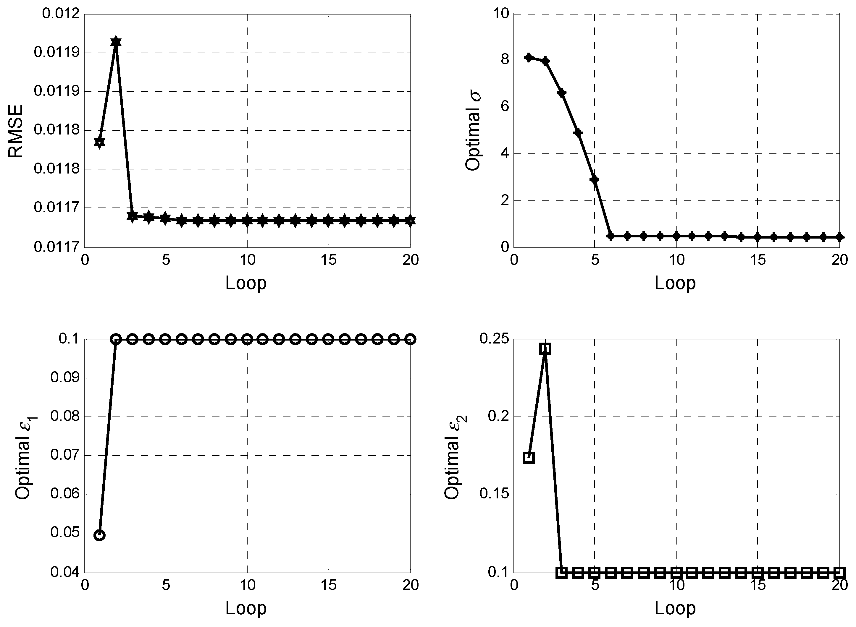
The number of particles in PSO is set to 20, as is the number of iteration. The initial particle’s positions and velocities are assumed randomly distributed within a given range. Figure 2 presents the results of RMSE, σ, ε1 and ε2. As can be seen from the results, the fitness and the parameters converge to stable values, obtained as RSME = 0.0117 , σ = 0.4356 , ε 1 = ε 2 = 0.1 . The three parameters, i.e., σ, ε1 and ε2, are used in the SVM based controller.
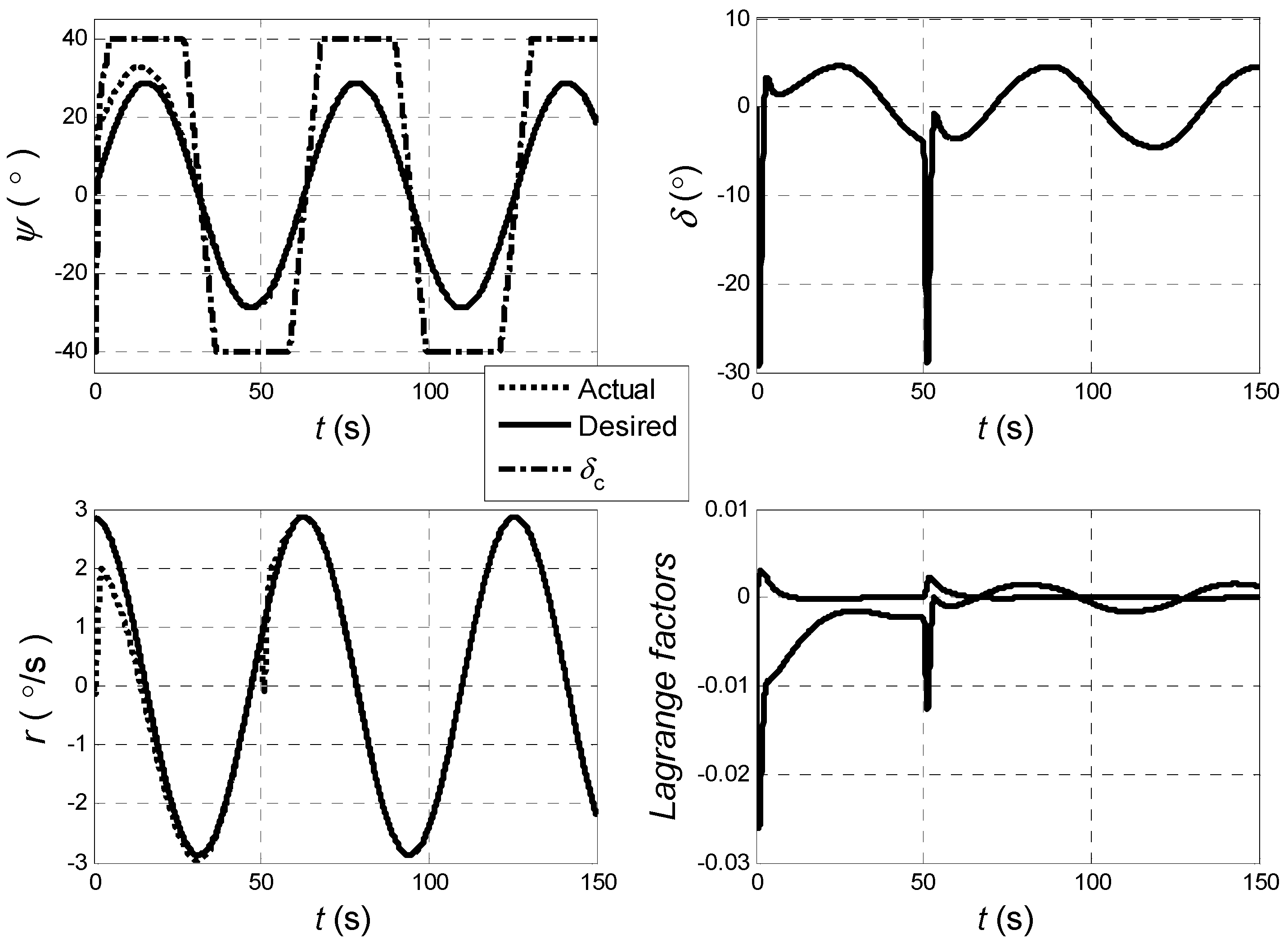
In the study, the control objective is to track a desired heading angle. Without loss of generality, the desired heading angle ψ d is assumed as a harmonic signal. To verify the stability and robustness of the controller designed, deviation of the heading angle is assumed at the start, which indicates that ψ ( t = 0 ) ψ d ( t = 0 ) . For uncertainties, the modeling error is assumed Δ ( ψ , ψ ˙ ) = ζ and the external disturbance is assumed as an instantaneous impulse with the amplitude of 1.5 (°/s) at the time 50 s t 51 s . Figure 3 presents the tracking results, including the histories of heading angle ψ , yaw rate r , demand rudder angle δ C , actual rudder angle δ , and Lagrangian factors ( α , β ) as well.
From the simulation results, it can be seen that both stability and robustness of the tracking system are achieved. The tracking accuracy is satisfactory as well. Moreover, the control inputs are reasonable and applicable from the point of view of operation.
As a comparison, a conventional PD controller is designed as follows,
δ c = k 1 e + k 2 e ˙
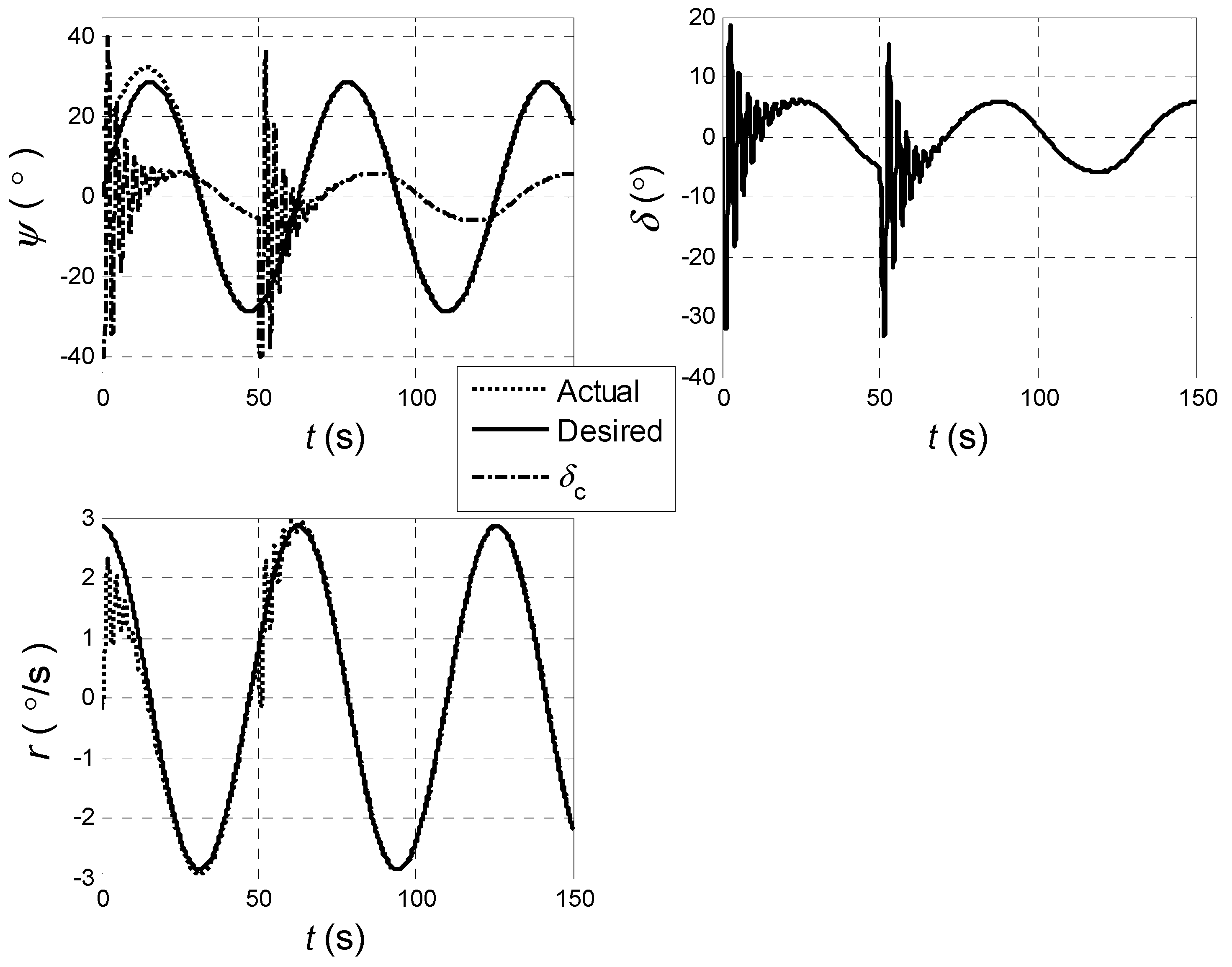
where k1,2 are control gains, selected as k1 = 5, k2 = 50. Figure 4 presents the simulation results using the PD controller designed. Compared with the performance of the SVM based controller as shown in Figure 3, it can be seen that obvious oscillation happens to the command rudder angle for a PD controller, which implies a limitation for the PD controller from an operational point of view despite the simple structure of the PD controller.
Further comparison is carried out by combining the SVM identification and inverse dynamic compensation that is commonly employed to obtain a feedback controller for a certain system (without uncertainties). By observing the inequality (24), the auxiliary controllers u1 and u2 can be designed as
u 1 = T λ e ˙ f ( ψ , ψ ˙ ) e ˙ + e + 1 4 μ 1 2 ζ + r 2 2 ζ 2 r 2 2 λ e + i = 1 2 α i K ( x i , x ) + λ 1 T ζ , ( λ 1 > 0 ) u 2 = K ζ ξ + i = 1 2 β i K ( x i , x ) + λ 2 T E ξ , ( λ 2 > 0 ) }
which indicates that only the modeling errors Δ ( ψ , ψ ˙ ) and the derivative of desired rudder angle δ d in the inequality (20) are approximated by SVM, i.e.,
Δ ( ψ , ψ ˙ ) = i = 1 l 1 α i K ( x i , x ) + η 1
T E δ ˙ d = i = 1 l 2 β i K ( x i , x ) + η 2
The terminal control input can be defined as
δ c = ( T ψ ¨ d + f ψ ˙ d + T λ e ˙ f ( ψ , ψ ˙ ) e ˙ + e + 1 4 μ 1 2 ζ + r 2 2 ζ 2 r 2 2 λ e + i = 1 2 α i K ( x i , x ) + λ 1 T ζ ) / K + K ζ ξ + i = 1 2 β i K ( x i , x ) + λ 2 T E ξ
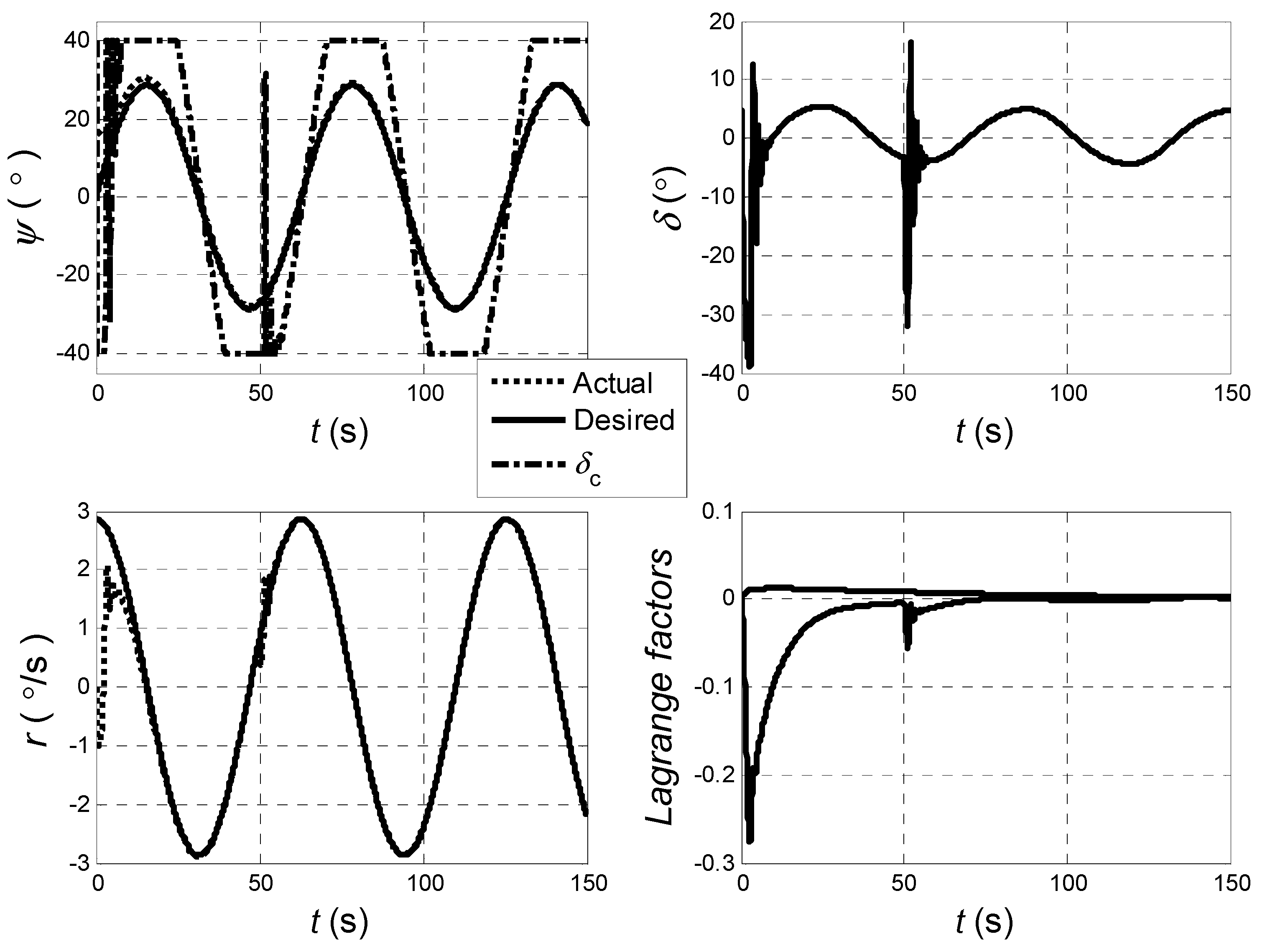
Comparing controller (54) with (31), one can find that the controller with inverse dynamic compensation in combination with SVM identification (given by (54)) is more complicated than the controller in which the complicated nonlinear function are indentified by SVM (given by (31)). Figure 5 presents the simulation results using controller (54). The parameters are selected as μ 1 = 0.25 , r 2 = 1 . In comparison with the results shown in Figure 3, it can be seen that oscillation of the command rudder angle happens at the initial stage and at the time of instantaneous external disturbance despite rapid convergence. Further remarks can be made as follows: (i) no matter whether inverse dynamic compensation is incorporated, the stability and robustness of the control system can be guaranteed due to the use of Lyapunov theory and L2-gain design; (ii) although the response rate of the controller in the case of inverse dynamic compensation (as described by (54)) is better than the case without compensation (as described by (31)), a moderate helming as shown in Figure 3, which can be achieved by using the controller (31), is preferable from the practical point of view. Moreover, as can be seen, the structure of the controller (31) is simpler than the controller (54), which makes sense in practice.

5. Conclusions

In this paper, SVM is applied to the control of a cascaded system with uncertainties with regard to ship course-keeping. The dynamics of the rudder actuator are considered in the plant. To guarantee the real-time performance of the controller, the Lagrangian factors in SVM are determined by on-line tuning algorithms. There are two advantages of the on-line SVM proposed in this paper over conventional on-line SVM. First, no supervised signal is required; second, the capacity of the training samples can be small, which improves the efficiency of the learning machine. Nonlinear functions and an uncertainty (modeling error) in the plant can be effectively identified by the proposed SVM, which helps obtain a controller with simple structure. Another method, L2-gain design, is applied to suppress the disturbance to the plant. The validity of the hybrid controller based on SVM and L2-gain design is confirmed by numerical simulation.
PSO is used to obtain the parameters in SVM. It should be noted that the optimal parameters are actually obtained in off-line way instead of on-line way, which limits its practical application to real-time control. In the next work, an on-line approach to the selection of SVM parameters will be studied.

Acknowledgments

This work was partially supported by the National Natural Science Foundation of China (No. 51505087), the Special Item supported by the Fujian Provincial Department of Ocean and Fisheries (No. MHGX-16), and the Special Item for University in Fujian Province supported by the Education Department (No. JK15003).

Author Contributions

Weilin Luo and Hongchao Cong analyzed the data; Weilin Luo wrote the paper.

Conflicts of Interest

The authors declare no conflict of interest.

References

  1. Perez, T. Ship Motion Control-Course Keeping and Roll Stabilization Using Rudder and Fins; Springer-Verlag London Ltd.: London, UK, 2005. [Google Scholar]
  2. Perera, L.P.; Guedes Soares, C. Pre-filtered Sliding Mode Control for Nonlinear Ship Steering Associated with Disturbances. Ocean Eng. 2012, 51, 49–62. [Google Scholar] [CrossRef]
  3. Carletti, C.; Gasparri, A.; Longhi, S.; UliviVapnik, G. Simultaneous Roll Damping and Course Keeping via Sliding Mode Control for a Marine Vessel in Seaway. In Proceedings of the 18th IFAC World Congress, Milano, Italy, 28 August–2 September 2011.
  4. Fossen, T.I. Guidance and Control of Ocean Vehicles; John Wiley & Sons: New York, NY, USA, 1994. [Google Scholar]
  5. Do, K.D. Global Robust and Adaptive Output Feedback Dynamic Positioning of Surface Ships. J. Mar. Sci. Appl. 2011, 10, 325–332. [Google Scholar] [CrossRef]
  6. Zwierzewicz, Z. On the ship course-keeping control system design by using robust and adaptive control. In Proceedings of the 19th International Conference on Methods and Models in Automation and Robotics (MMAR), Miedzyzdroje, Poland, 2–5 September 2014; pp. 189–194.
  7. Katebi, M.R.; Grimble, M.J.; Zhang, Y. H∞ Robust Control Design for Dynamic Ship Positioning. IEE Proc. Control Theory Appl. 2011, 114, 110–120. [Google Scholar] [CrossRef]
  8. Unar, M.A.; Murray-Smith, D.J. Automatic Steering of Ships Using Neural Networks. Int. J. Adapt. Control Signal Process. 1999, 13, 203–218. [Google Scholar] [CrossRef]
  9. Xu, H.; Li, W.; Yu, Y.; Liu, Y. A novel adaptive neural control scheme for uncertain ship course-keeping system. Sens. Transducers 2014, 178, 282–285. [Google Scholar]
  10. Ren, J.; Zhang, X. Ship course-keeping adaptive Fuzzy controller design using command filtering with minimal parametrization. In Proceedings of the 25th Chinese Control and Decision Conference (CCDC), Guiyang, China, 25–27 May 2013; pp. 243–247.
  11. Velagica, J.; Vukicb, Z.; Omerdic, E. Adaptive Fuzzy Ship Autopilot for Track-Keeping. Control Eng. Pract. 2007, 34, 2074–2085. [Google Scholar] [CrossRef]
  12. Borkowski, P. Ship course stabilization by feedback linearization with adaptive object model. Pol. Marit. Res. 2014, 21, 14–19. [Google Scholar] [CrossRef]
  13. Fang, M.C.; Lee, Z.Y. Application of neuro-fuzzy algorithm to portable dynamic positioning control system for ships. Int. J. Nav. Arch. Ocean Eng. 2016, 8, 38–52. [Google Scholar] [CrossRef]
  14. Moreiraa, L.; Fossen, T.I.; Guedes Soares, C. Path Following Control System for a Tanker Ship Model. Ocean Eng. 2007, 16, 479–489. [Google Scholar] [CrossRef]
  15. Oh, S.-R.; Sun, J. Path Following of Underactuated Marine Surface Vessels Using Line-of-Sight Based Model Predictive Control. Ocean Eng. 2010, 37, 289–295. [Google Scholar] [CrossRef]
  16. Zwierzewicz, Z. The Design of ship autopilot by applying observer-based feedback linearization. Pol. Marit. Res. 2015, 22, 16–21. [Google Scholar] [CrossRef]
  17. Le, M.D.; Nguyen, S.H.; Nguyen, L.A. Study on a new and effective fuzzy PID ship autopilot. Artif. Life Robot. 2004, 8, 197–201. [Google Scholar] [CrossRef]
  18. Sun, X.; Chen, W. Global generalised exponential/finite-time control for course-keeping of ships. Int. J. Control 2016, 89, 1169–1179. [Google Scholar] [CrossRef]
  19. Blank, M.; Lindegaard, K.P.; Fossen, T.I. Dynamic model for thrust generation of marine propellers. In Proceedings of the Conference on Manoeuvring Control Marine Craft, Aalborg, Denmark, 23–25 August 2000; pp. 363–368.
  20. Pend, X.; Jia, S.; Hu, Z. Nonlinear H-infinity inverse optimal output feedback control for ship course. Control Theory Appl. 2014, 31, 215–222. [Google Scholar]
  21. Alfi, A.; Shokrzadeh, A.; Asadi, M. Reliability analysis of H-infinity control for a container ship in way-point tracking. Appl. Ocean Res. 2015, 52, 309–316. [Google Scholar] [CrossRef]
  22. Zhao, J.; Li, P.; Wang, X.S. Intelligent PID controller design with adaptive criterion adjustment via least squares support vector machine. In Proceedings of the 21th Chinese Control and Decision Conference, Guilin, China, 17–19 June 2009.
  23. Ahmed, Y.A.; Kazuhiko, H. Automatic ship berthing using artificial neural network trained by consistent teaching data using nonlinear programming method. Eng. Appl. Artif. Intell. 2013, 26, 2287–2304. [Google Scholar] [CrossRef]
  24. Lisowski, J. Multi-stage safe ship control with neural state constraints. In Proceedings of the 2015 IEEE 2nd International Conference on Cybernetics (CYBCONF), Gdynia, Poland, 24–26 June 2015; pp. 56–61.
  25. Vapnik, V.N. Statistical Learning Theory; John Wiley & Sons: New York, NY, USA, 1998. [Google Scholar]
  26. Liu, S.; Wang, Y.C.; Fu, H.X. Variable universe fuzzy-least squares support-vector-machine compound control for ship course-keeping. Control Theory Appl. 2011, 28, 485–490. [Google Scholar]
  27. Jiang, S.Q.; Jin, H.Z.; Wei, F.M. LS-SVM application for ship course model predictive control. In Proceedings of the 2013 IEEE International Conference on Mechatroncis and Automation, Takamatsu, Japan, 4–7 August 2013; pp. 1615–1619.
  28. Luo, W.L.; Fu, B.; Guedes Soares, C.; Zou, Z.J. Robust control for ship course-keeping based on support vector machines: Particle swarm optimization and L2-gain. In Proceedings of the 32nd International Conference on Ocean, Offshore and Arctic Engineering, Nantes, France, 9–14 June 2013.
  29. Fossen, T.I. Handbook of Marine Craft Hydrodynamics and Motion Control; John Wiley & Sons: New York, NY, USA, 2011. [Google Scholar]
  30. Suykens, J.A.; Vandewalle, J.; De Moor, B. Optimal control by least squares support vector machines. Neural Netw. 2001, 14, 23–35. [Google Scholar] [CrossRef]
  31. Suykens, J.A.K.; De Brabanter, J.; Lukas, L.; Vandewalle, J. Weighted least squares support vector machines: Robustness and sparse approximation. Neurocomputing 2002, 48, 85–105. [Google Scholar] [CrossRef]
  32. Vapnik, V.N.; Esther, L.E.; Lecun, Y. Measuring the VC-Dimension of a Learning Machine. Neural Comput. 1994, 6, 851–876. [Google Scholar] [CrossRef]
  33. Cherkassky, V.; Ma, Y. Practical selection of SVM parameters and noise estimation for SVM regression. Neural Netw. 2004, 17, 113–126. [Google Scholar] [CrossRef]
  34. Anguita, D.; Oneto, L. In-sample and out-of-sample model selection and error estimation for support vector machines. IEEE Trans. Neural Netw. Learn. Syst. 2012, 23, 1390–1406. [Google Scholar] [CrossRef] [PubMed]
  35. Zhao, W.; Tao, T.; Ding, Z.; Zio, E. A dynamic particle filter-support vector regression method for reliability prediction. Reliab. Eng. Syst. Saf. 2013, 119, 109–116. [Google Scholar]
  36. Kennedy, J.; Eberhart, R. Particle Swarm Optimization. In Proceedings of the IEEE International Conference on Neural Networks, Perth, WA, USA, 27 November–1 December 1995; Volume 4, pp. 1942–1948.
  37. Ranaee, V.; Ebrahimzadeh, A.; Ghaderi, G. Application of the PSO-SVM model for recognition of control chart patterns. ISA Trans. 2010, 49, 577–586. [Google Scholar] [CrossRef] [PubMed]
  38. Selakova, A.; Cvijetinovic, D.; Milovic, L.; Mellonb, S.; Bekutc, D. Hybrid PSO–SVM method for short-term load forecasting during periods with significant temperature variations in city of Burbank. Appl. Soft Comput. 2014, 16, 80–88. [Google Scholar] [CrossRef]
  39. García Nieto, P.J.; García-Gonzalo, E.; Sánchez Lasheras, F.; de Cos Juez, F.J. Hybrid PSO–SVM-based method for forecasting of the remaining useful life for aircraft engines and evaluation of its reliability. Reliab. Eng. Syst. Safety 2015, 138, 219–231. [Google Scholar] [CrossRef]
  40. Wang, D.; Huang, J. Adaptive neural network control for a class of uncertain nonlinear systems in pure-feedback form. Automatica 2002, 38, 1365–1372. [Google Scholar] [CrossRef]
  41. Luo, W.L.; Zou, Z.J. Identification of response models of ship maneuvering motion using support vector machines. J. Ship Mech. 2007, 12, 832–838. [Google Scholar]
Figure 1. Control framework.
Algorithms 09 00052 g001
Figure 2. Parameter optimization by PSO.
Algorithms 09 00052 g002
Figure 3. Simulation results using an SVM-based controller.
Algorithms 09 00052 g003
Figure 4. Simulation results using PD controller.
Algorithms 09 00052 g004
Figure 5. Simulation results using SVM controller in combination of inverse dynamic compensation.
Algorithms 09 00052 g005