Abstract
Low-Rank Tensor Recovery (LRTR), the higher order generalization of Low-Rank Matrix Recovery (LRMR), is especially suitable for analyzing multi-linear data with gross corruptions, outliers and missing values, and it attracts broad attention in the fields of computer vision, machine learning and data mining. This paper considers a generalized model of LRTR and attempts to recover simultaneously the low-rank, the sparse, and the small disturbance components from partial entries of a given data tensor. Specifically, we first describe generalized LRTR as a tensor nuclear norm optimization problem that minimizes a weighted combination of the tensor nuclear norm, the l1-norm and the Frobenius norm under linear constraints. Then, the technique of Alternating Direction Method of Multipliers (ADMM) is employed to solve the proposed minimization problem. Next, we discuss the weak convergence of the proposed iterative algorithm. Finally, experimental results on synthetic and real-world datasets validate the efficiency and effectiveness of the proposed method.
1. Introduction
In the past decade, the low-rank property of some datasets has been explored skillfully to recover both the low-rank and the sparse components or complete the missing entries. The datasets to be analyzed are usually modeled by matrices and the corresponding recovery technique is named as Low-Rank Matrix Recovery (LRMR). LRMR has received a significant amount of attention in some fields of information science such as computer vision, machine learning, pattern recognition, data mining and linear system identification. There are several appealing types of LRMR including Matrix Completion (MC) [1], Robust Principal Component Analysis (RPCA) [2] and Low-Rank Representation (LRR) [3]. Mathematically, we customarily formulate LRMR as matrix nuclear norm minimization problems that can be effectively solved by several scalable methods. Diverse variants of LRMR derive from the aforementioned three models, for instance, MC with noise (or stable MC) [4], stable RPCA [5,6], incomplete RPCA [7], LRR with missing entries [8], and LRMR based on matrix factorization or tri-factorization [9,10].
The fields of image and signal processing usually require processing large amounts of multi-way data, such as video sequences, functional magnetic resonance imaging sequences and direct-sequence code-division multiple access (DS-CDMA) systems [11]. For the datasets with multi-linear structure, traditional matrix-based data analysis is prone to destroy the spatial and temporal structure, and can be affected by the curse of dimensionality. In contrast, tensor-based data representation can avoid or alleviate the above deficiencies to some extent. Furthermore, tensor decompositions can be used to obtain a low-rank approximation of an investigated data tensor. Two of the most popular tensor decompositions are the Tucker model and the PARAFAC (Parallel Factor Analysis) model, and they can be thought of as the higher order generalizations of Singular Value Decomposition (SVD) and Principal Component Analysis (PCA) [12].
Generally speaking, the traditional tensor decomposition models are very sensitive to missing entries, arbitrary outliers and gross corruptions. On the contrary, Low-Rank Tensor Recovery (LRTR) is very effective to recover simultaneously the low-rank component and the sparse noise, or complete the missing entries. As the higher order generalization of LRMR, LRTR is composed mainly of tensor completion [13] and Multi-linear RPCA (MRPCA) [14]. The task of tensor completion is to recover missing or unsampled entries according to the low-rank structure. The alternating least squares method based on the PARAFAC decomposition was originally proposed to complete missing entries [15]. Subsequently, the Tucker decomposition was applied to the problem of tensor completion [16,17,18]. The multi-linear rank is commonly used to describe the low-rank property, although it is hard to be properly estimated. The tensor nuclear norm generalizes the matrix nuclear norm and becomes a new standard for measuring the low-rank structure of a tensor. Hence, LRTR can usually be boiled down to a tensor nuclear norm minimization problem.
Liu et al. [13] established a tensor nuclear norm minimization model for tensor completion and proposed the Alternating Direction Method of Multipliers (ADMM) for efficiently solving this model. Gandy et al. [19] considered the low-n-rank tensor recovery problem with some linear constraints and developed the Douglas–Rachford splitting technique, a dual variant of the ADMM. To reduce the computational complexity of the tensor nuclear norm minimization problems, Liu et al. [20] introduced the matrix factorization idea into the minimization model and obtained a much smaller matrix nuclear norm minimization problem. Tan et al. [21] transformed tensor completion into a linear least squares problem and proposed a nonlinear Gauss–Seidel method to solve the corresponding optimization problem. In [14], Shi et al. extended RPCA to the case of tensors and presented the MRPCA model. MRPCA, also named robust low-rank tensor recovery [22], was described as a tensor nuclear norm minimization which can be solved efficiently by the ADMM.
This paper studies a generalized model of LRTR. In this model, the investigated data tensor is assumed to be the superposition of a low-rank component, a gross sparse tensor and a small dense error tensor. The Generalized Low-Rank Tensor Recovery (GLRTR) aims mainly to recover the low-rank and the sparse components from partially observed entries. For this purpose, we establish a tensor nuclear norm minimization model for GLRTR. In addition, the ADMM method is adopted to solve the proposed convex model.
The rest of this paper is organized as follows. Section 2 provides mathematical notations and introduces preliminaries on tensor algebra. In Section 3, we review related works on LRTR. We present a generalized LRTR model and develop an efficient iterative algorithm for solving the proposed model in Section 4. Section 5 discusses the weak convergence result on the proposed algorithm. We report the experimental results in Section 6. Finally, Section 7 draws the conclusions.
2. Notations and Preliminaries
This section will briefly introduce mathematical notations and review tensor algebra. We denote tensors by boldface Euclid Math One, e.g., , matrices by boldface capital letters, e.g., A, vectors by boldface letters, e.g., a, and scalars by italic letters, e.g., a or A. A tensor with order N indicates that its entries can be expressed via N indices. For an Nth-order real tensor , its entry is denoted by .
The n-mode matricization (unfolding) of tensor , denoted by , is an matrix obtained by rearranging n-mode fibers to be the columns of the resulting matrix. Furthermore, we define an opposite operation “fold” as . Given another tensor , the inner product between and is defined as . Then, the Frobenius norm (or l2-norm) of tensor can be induced by the above inner product, that is, . Moreover, we also give other norm definitions of a tensor, which will be needed in the following sections. The l1-norm of tensor is expressed as and the tensor nuclear norm is , where , named the nuclear norm of , is the sum of singular values of and . Due to the fact that the nuclear norm of one matrix is the tightest convex relaxation of the rank function on the unit ball in the spectral norm, it is easy to verify that the tensor nuclear norm is a convex function with respect to .
The n-mode product of tensor by a matrix , denoted as , is an Nth-order tensor with the dimensionality of , and its entry is calculated as . The multi-linear rank of tensor is stipulated as a vector , where indicates the rank function of a matrix. Tensor is low-rank if and only if for some n. Then, the Tucker decomposition of is defined as
where the core tensor , mode matrices and . The multi-linear rank of a tensor has superiority over other definitions (e.g., the rank used in PARAFAC decomposition) because it is easy to compute. Refer to the survey [12] for further understanding of tensor algebra.
Within the field of low-rank matrix/tensor recovery, two proximal minimization problems are extensively employed:
where and A are a given data tensor and matrix respectively, is a regularization factor. To address the above two optimization problems, we first define an absolute thresholding operator as below: . It has been proven that problems (2) and (3) have closed-form solutions denoted by [2] and [23] respectively, where and is the singular value decomposition of A.
3. Related Works
Tensor completion and MRPCA are two important and appealing applications of LRTR. In this section, we review the related works on the aforementioned two applications.
As the higher order generalization of matrix completion, tensor completion aims to recover all missing entries with the aid of the low-rank (or approximately low-rank) structure of a data tensor. Although low-rank tensor decompositions are practical in dealing with missing values [15,16,17,18], we have to estimate properly the rank of an incomplete tensor in advance. In the past few years, the matrix nuclear norm minimization model has been extended to the tensor case [13]. Given an incomplete data tensor and a corresponding sampling index set , we define a linear operator as follows: if , ; otherwise, , where . Then, the original tensor nuclear norm minimization model for tensor completion [13] is described as:
To tackle problem (4), Liu et al. [13] developed three different algorithms and demonstrated experimentally that the ADMM is the most efficient algorithm in obtaining a high accuracy solution. If we further take the dense Gaussian noise into consideration, then the stable version of tensor completion is given as below [19]:
or its corresponding unconstrained formulation:
where the regularized parameter is used to balance the low-rankness and the approximate error, and η is a known estimate of the noise level.
In RPCA, a data matrix is decomposed into the sum of a low-rank component and a sparse component, and it is possible to recover simultaneously the two components by principal component pursuit under some suitable assumptions [2]. Shi et al. [14] extended RPCA to the case of tensors and presented the framework of MRPCA, which regards the data tensor as the sum of a low-rank tensor and a sparse noise term . Mathematically, the low-rank and the sparse components can be simultaneously recovered by solving the following tensor nuclear norm minimization problem:
In [22], MRPCA is also called as robust low-rank tensor recovery.
4. Generalized Low-Rank Tensor Recovery
Both tensor completion and MRPCA do not consider dense Gaussian noise corruptions. In this section, we investigate the model of Generalized Low-Rank Tensor Recovery (GLRTR) and develop a corresponding iterative scheme.
4.1. Model of GLRTR
The datasets contaminated by Gaussian noise are very universal in practical engineering applications. In view of this, we assume the data tensor to be the superposition of the low-rank component , the large sparse corruption and the Gaussian noise . We also consider the case that some entries of are missing. To recover simultaneously the above three terms, we establish a convex GLRTR model as follows:
where the regularization coefficients λ and τ are nonnegative.
If we reinforce the constraints (or equivalently ) and (or equivalently ), then the GLRTR is transformed into the tensor completion model (4), where the zero tensor has the same dimensionality as . If only the constraint is considered, then the GLRTR is equivalent to Equation (6). Furthermore, if we take and , then the model of GLRTR becomes the model of MRPCA. In summary, the proposed model is the generalization of the existing LRTR.
For the convenience of using the splitting method, we discard and introduce N + 1 auxiliary tensor variables , where these auxiliary variables have the same dimensionality as . Let be the n-mode matricization of for each and . Hence, we have the equivalent formulation of Equation (8):
As a matter of fact, the discarded low-rank tensor can be represented by . Now, we explain the low-rankness of from two viewpoints. One is . The other is that a better solution to Equation (9) will satisfy . These viewpoints illustrate that is approximately low-rank along each mode. The aforementioned non-smooth minimization problem is distributed convex. Concretely speaking, the tensor variables can be split into several parts and the objective function is separable across this splitting.
4.2. Optimization Algorithm to GLRTR
As a special splitting method, the ADMM is very efficient to solve a distributed optimization problem with linear equality constraints. It takes the form of the decomposition–coordination procedure and blends the merits of dual decomposition and augmented Lagrangian methods. In this section, we will propose the method of ADMM to solve Equation (9).
We first construct the augmented Lagrangian function of the aforementioned convex optimization problem without considering the constraint :
where μ is a positive numerical constant, are Lagrangian multiplier tensors and . There are totally five blocks of variables in . The ADMM algorithm updates alternatively each block of variables while letting the other blocks of variables be fixed. If is given, one block of variables in can be updated by minimizing with respect to one argument. On the contrary, if are given, is updated by maximizing with respect to . The detailed iterative procedure is outlined as follows:
Computing . Fix and minimize with respect to :
where . In consideration of the constraint , the final update formulation of is revised as
where is the complement set of Ω.
Computing . If is unknown and other variables are fixed, we update by minimizing with respect to :
where and is the n-mode matricization of .
Computing . If is unknown and other variables are fixed, the calculation procedure of is given as follows:
Computing . The update formulation of is calculated as
Computing . If are fixed, we can update the Lagrangian multipliers as follows:
Once are updated, we will increase the value of μ by multiplying it with a constant during the procedure of iterations. The whole iterative procedure is outlined in Algorithm 1. The stopping condition of Algorithm 1 is set as or the maximum number of iterations is reached, where ε is a sufficiently small positive number.
| Algorithm 1. Solving GLRTR by ADMM |
| Input: Data tensor , sampling index set Ω, regularization parameters λ and τ. |
| Initialize: and ρ. |
| Output: and . |
While not converged do
|
| End while |
In our implementation, and are initialized to zeros tensors. The other parameters are set as follows: and Furthermore, the maximum number of iterations is set to 100.
5. Convergence Analysis
Because the number of block variables in Equation (9) is more than two, it is difficult for us to prove the convergence of Algorithm 1. Nevertheless, the experimental results in the next section demonstrate this algorithm has good convergence behavior. This section will discuss the weak convergence result on our ADMM algorithm.
We consider a special case of Algorithm 1, that is, there is no missing entries. In this case, it holds that . Thus, Equation (9) is transformed into
We can design a corresponding ADMM algorithm by revising Algorithm 1, namely, the update formulation of is replaced by . In fact, the revised algorithm is an inexact version of ADMM. Subsequently, we give the iterative formulations of exact ADMM for Equation (17):
In this circumstance, we have the following statement:
Theorem 1.
Let be the sequence produced by (18). If has a saddle point with respect to , then satisfy that the iterative sequence of objective function in Equation (17) converges to the minimum value.
Proof.
By matricizing each tensor along the one-mode, the constraints of Equation (17) can be rewritten as a linear equation:
or equivalently,
where I is an identity matrix of size I1 × I1. If we integrate and into one block of variables, then Equation (20) is re-expressed as below:
We denote and partition all variables in Equation (17) into two parts in form of matrices: M and . Essentially, and are the matricizations of and , respectively. Let . Then, the objective function in Equation (17) can be expressed as . It is obvious that and are two closed, proper and convex functions. According to the basic convergence result given in [24], we have , where is the minimum value of under the linear Constraint (21). This ends the proof. □
In the following, we discuss the detailed iterative procedure of or in Equation (18). It is easy to verify that the update formulation of in Equation (18) is equivalent to:
The block of variables can be solved in parallel because the objective function in Equation (22) is separable with respect to . Hence, the iterative formulation of is similar to that of Equation (13).
For fixed M and , we can get the optimal block of variables or by minimizing , where . The partial derivative of with respect to is
By letting , we have
where . By substituting Equation (24) into , we have the update formulation of :
A standard extension of the classic ADMM is to use varying parameter μ for each iteration. The goal of this extension is to improve the convergence and reduce the dependence on the initial choice of μ. In the context of the method of multipliers, this approach is proven to be superlinearly convergent if [25], which inspires us to adopt the non-decreasing sequence . Furthermore, large values of μ result in a large penalty on violations of primal feasibility and are thus inclined to produce small primal residuals. However, it is difficult to prove the convergence of ADMM [24]. A commonly-used choice for is , where and is the upper limit of μ. Due to the fact that is fixed after a finite number of iterations, the corresponding ADMM is convergent according to Theorem 1.
6. Experimental Results
We perform experiments on synthetic data and two real-world video sequences, and validate the feasibility and effectiveness of the proposed method. The experimental results of GLRTR are compared with that of MRPCA, where the missing values in MRCPA are replaced by zeros.
6.1. Synthetic Data
In this subsection, we synthesize data tensors with missing entries. First, we generate an Nth-order low-rank tensor as follows: with the core tensor and mode matrices . The entries of and are independently drawn from the standard normal distribution. Then, we generate randomly a dense noise tensor whose entries also obey the standard normal distribution. Next, we construct a sparse noise tensor , where is produced by a uniform distribution on the interval and the index set is produced by uniformly sampling on with probability p′%. Finally, the generation of the sampling index set Ω is similar to Ω′ and the corresponding sampling rate is set to be p%. Therefore, an incomplete data tensor is synthesized as .
For given data tensor with missing values, its low-rank component recovered by some method is denoted by . The Relative Error (RE) is employed to evaluate the recovery performance of the low-rank structure and its definition is given as follows: . Small relative error means good recovery performance. The experiments are carried out on 50 × 50 × 50 tensors and 20 × 20 × 20 × 20 tensors, respectively. Furthermore, we set a = 500 and .
For convenience of comparison, we design three groups of experiments. In the first group of experiments, we only consider the case that there are no missing entries, that is, or p = 100. The values of and are adopted to indicate the Inverse Signal-to-Noise Ratio (ISNR) with respect to the sparse and the Gaussian noise respectively. Three different degrees of sparsity are taken into account, that is, p′ = 5, 10 and 15. In addition, we take for 3rd-order tensors and for 4th-order tensors. For given parameters, we repeat the experiments ten times and report the average results. As a low-rank approximation method for tensors, the Higher-Order SVD (HOSVD) truncation [12] to rank- is not suitable for gross corruptions owing to the fact that its relative error reaches up to 97% or even 100%. Hence, we do not compare this method with our GLRTR in subsequent experiments. The experimental results are shown in Table 1 and Table 2, respectively.

Table 1.
Comparison of experimental results on 50 × 50 × 50 tensors.
Table 2.
Comparison of experimental results on 20 × 20 × 20 × 20 tensors.
From the above two tables, we have the following observations: (I) Although the values of ISNR on sparse noise are very large, both MRPCA and GLRTR remove efficiently sparse noise to some extent. Meanwhile, large values of ISNR on Gaussian noise are disadvantageous for recovering the low-rank components; (II) GLRTR has better recovery performance than MRPCA. In an average sense, the relative error of GLRTR is 2.68% smaller than that of MRPCA for 50 × 50 × 50 tensors, and 14.17% for 20 × 20 × 20 × 20 tensors; (III) For 3rd-order tensors, GLRTR removes effectively Gaussian noise, and, on average, its relative error is 5.96% smaller than the value of ISNR on Gaussian noise; for 4th-order tensors, GLRTR effectively removes Gaussian noise only in the case r = 2. In summary, GLRTR is more effective than MRPCA in recovering the low-rank components.
The second group of experiments considers four different sampling rates for Ω and one fixed degree of sparsity for Ω′, that is, and p′ = 5. We set τ = 0.02 for both 3rd-order and 4th-order tensors, and choose the superior tradeoff parameter λ for each p. The comparisons of experimental results between MRPCA and GLRTR are shown in Table 3 and Table 4, respectively. We can see from these two tables that MRPCA is very sensitive to the sampling rate p%, and it hardly recovers the low-rank components. In contrast, GLRTR achieves better recovery performance for 3rd-order tensors. As for 4th-order tensors, it also has smaller relative error when the sampling rate p% is relatively large. These observations show that GLRTR is more robust to missing values than MRPCA.
Table 3.
Comparison of experimental results on incomplete 50 × 50 × 50 tensors for r = 5.
Table 4.
Comparison of experimental results on incomplete 20 × 20 × 20 × 20 tensors for r = 4.
We will evaluate the sensitivity of GLRTR to the choice of λ and τ in the last group of experiments. For convenience of designing experiments, we only perform experiments on 50 × 50 × 50 tensors and consider the case that p = 100. The values of λ and τ are set according to the following manner: we vary the value of one parameter while letting the other be fixed. In the first case, the parameter τ is chosen as 0.01. Under this circumstance, the relative errors versus different λ of MRPCA and GLRTR are shown in Figure 1. We take λ = 0.01 in the second case and the relative errors versus different τ of GLRTR are shown in Figure 2.
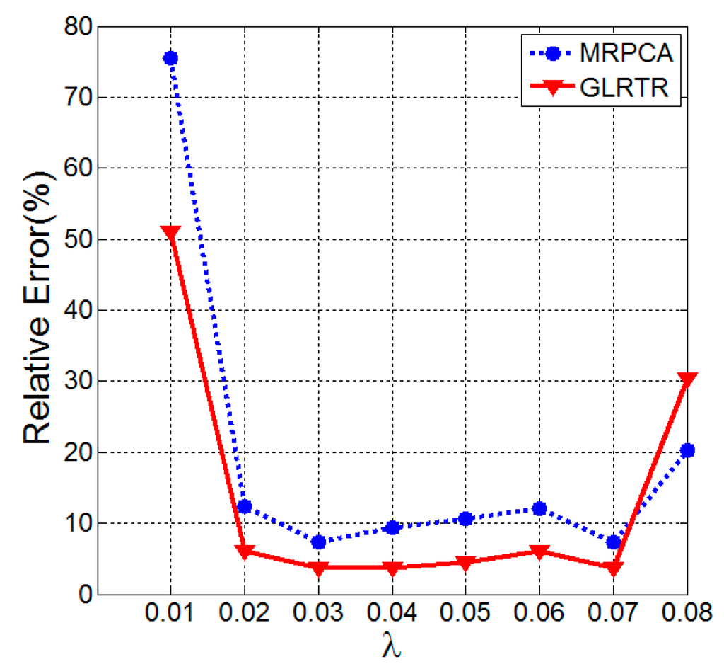
Figure 1.
Comparison of relative errors between Multi-linear Robust Principal Component Analysis (MRPCA) and Generalized Low-Rank Tensor Recovery (GLRTR) with varying λ.
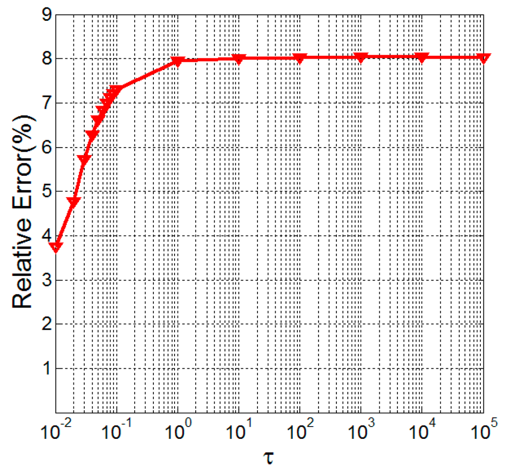
Figure 2.
Relative errors of Generalized Low-Rank Tensor Recovery (GLRTR) with varying τ.
It can be seen from Figure 1 that the relative errors of MRPCA and GLRTR are about 9.90% and 4.62%, respectively, if 0.02 ≤ λ ≤ 0.07, which means the latter has better recovery performance than the former. Furthermore, their relative errors are relatively stable when λ lies within a certain interval. Figure 2 illustrates that the relative error has the tendency to increase monotonically, and it becomes almost stationary when τ ≥ 1. At this moment, the relative errors lie in the interval (0.037, 0.080). This group of experiments implies that, for our synthetic data, GLRTR is not very sensitive to the choice of λ and τ.
6.2. Influence of Noise and Sampling Rate on the Relative Error
This subsection will evaluate the influence of noise and sampling rate on the relative error. For this purpose, we design four groups of experiments and use the synthetic data generated in the same manner as in the previous subsection. For the sake of convenience, we only carry out experiments on 50 × 50 × 50 tensors.
The first group of experiments aims to investigate the influence of noise on the recovery performance. In the data generation process, we only change the manner for generating , that is, each entry of is drawn independently from the normal distribution with mean zero and standard deviation b. Let and b = 0.2j, where . For different combinations of a and b, the relative errors of GLRTR are shown in Figure 3. We can draw two conclusions from this figure. For given b, the relative error is relatively stable with the increasing of a, which means the relative error is not very sensitive to the magnitude of sparse noise. The relative error monotonically increases with the increasing of Gaussian noise level, which validates that large Gaussian noise is disadvantageous for recovering the low-rank component.
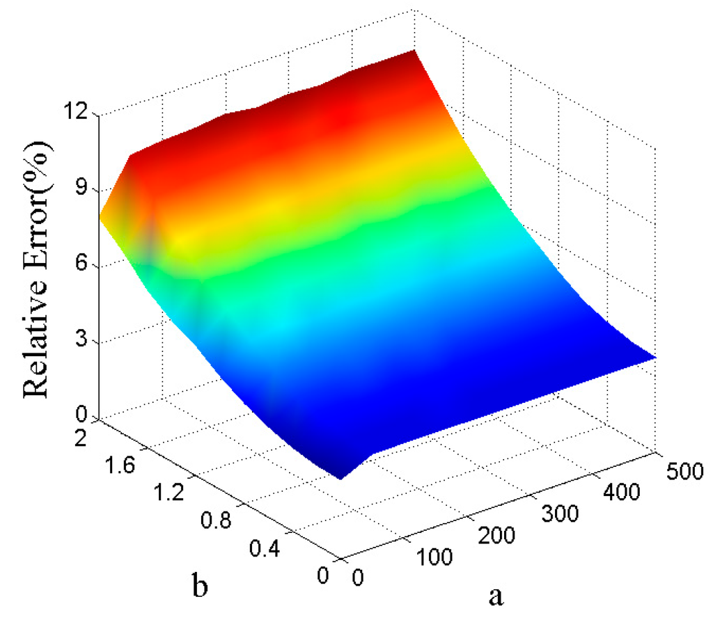
Figure 3.
Relative errors for different a and b.
Next, we study the influence of sampling rate p% on the relative error for different r. Set and vary the value of p% from 30 to 100 in steps of size 10. For fixed r and p, we obtain the low-rank component according to GLRTR and then plot the relative errors in Figure 4. From the 3-D colored surface in Figure 4, we can see that both r and p have significant influence on the relative error. This observation indicates that small r or large p is conducive to the recovery of low-rank term.
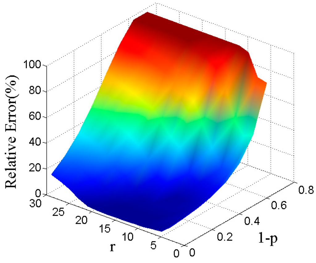
Figure 4.
Relative errors for different r and p.
The third group of experiments will validate the robustness of GLRTR to sparse noise. Concretely speaking, we investigate the recovery performance under different ISNR on sparse noise without consideration of Gaussian noise. Set , . The experimental results are shown in Figure 5, where the horizontal and the vertical coordinates represent the ISNR on sparse noise and the relative error, respectively. This figure illustrates that the relative error is less than 4.5% for synthetic 3rd-order tensors, which verifies experimentally that our method is very robust to sparse noise.
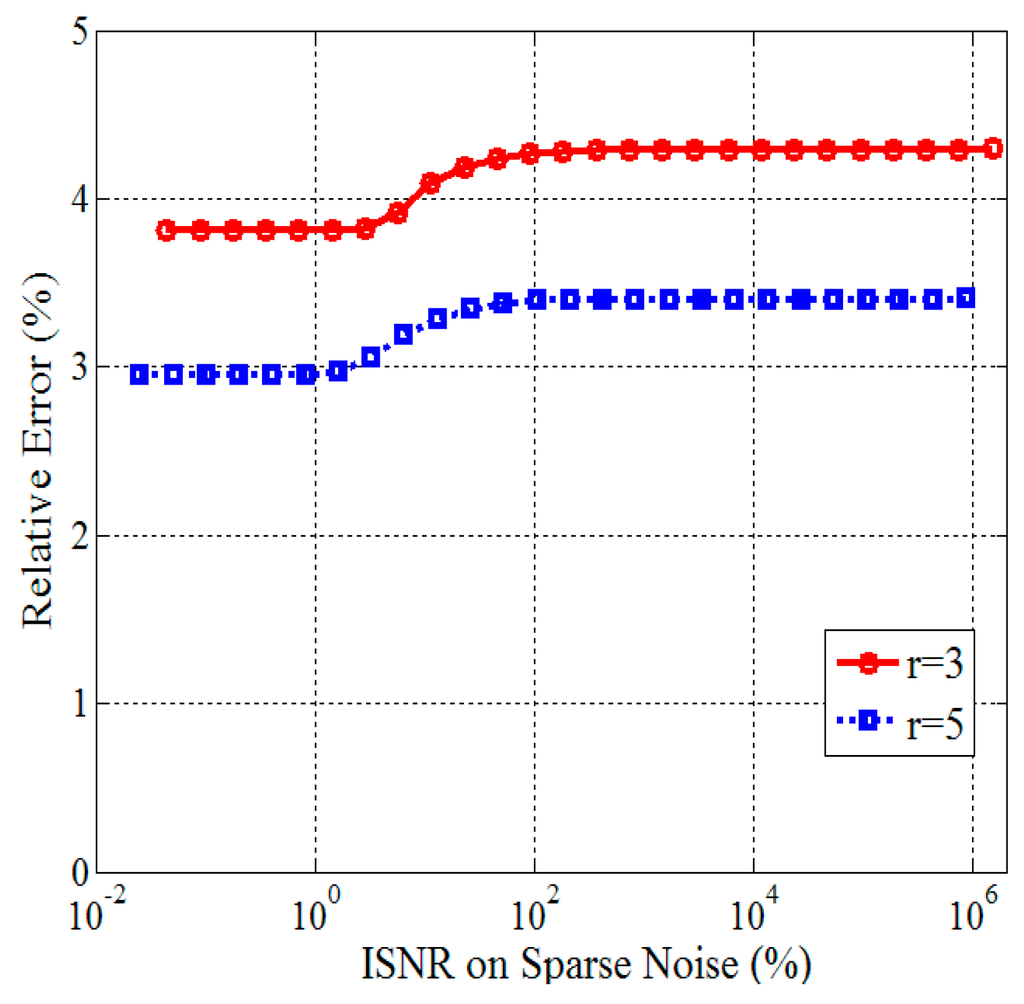
Figure 5.
Relative errors versus different Inverse Signal-to-Noise Ratio (ISNR) on sparse noise.
In the last group of experiments, we discuss the performance of GLRTR in removing the small dense noise for given large sparse noise. We also propose a combination strategy: GLRTR + HOSVD, that is, GLRTR is followed by HOSVD. The goal of this new method is to improve the denoising performance of GLRTR. Let and . Different values for b lead to different ISNR on Gaussian noise. We draw four curves to reflect the relationship between the relative error and ISNR on Gaussian noise, as shown in Figure 6, where the black dashed line is a reference line. We have two observations from this figure. When ISNR on Gaussian noise is larger than 3.5%, GLRTR not only successfully separates the sparse noise to some extent but also effectively removes the Gaussian noise. The GLRTR+HOSVD method has better denoising performance than GLRTR in the presence of large Gaussian noise.
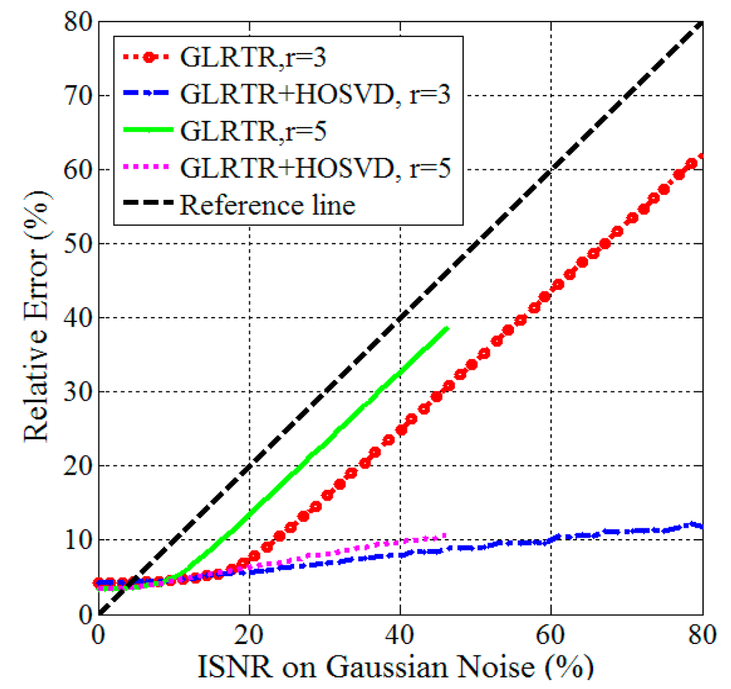
Figure 6.
Relative errors versus different Inverse Signal-to-Noise Ratio (ISNR) on Gaussian noise.
6.3. Applications in Background Modeling
In this subsection, we test our method on two real-world surveillance videos for object detection and background subtraction: Lobby and Bootstrap datasets [26]. For convenience of computation, we only consider the first 200 frames for each dataset and transform the color images into the gray-level images. The resolutions of each image in the Lobby and Bootstrap datasets are 128 × 160 and 120 × 160, respectively. We add Gaussian noise with mean zero and standard deviation 5 to each image. Hence, we obtain two data tensors of order 3 and their sizes are 128 × 160 × 200 and 120 × 160 × 200, respectively. For two given tensors, we execute random sampling on them with a probability of 50%.
Considering the fact that MRPCA fails in recovering the low-rank components on the synthetic data with missing values, we only implement the method of GLRTR on the video datasets. Two tradeoff parameters are set as follows: λ = 0.0072 and τ = 0.001. We can obtain the low-rank, the sparse and the completed components from the incomplete data tensors according to the proposed method. Actually, the low-rank terms are the backgrounds and the sparse noise terms correspond to the foregrounds. The experimental results are partially shown in Figure 7 and Figure 8, respectively, where the missing entries in incomplete images are shown in white. From Figure 7 and Figure 8, we can see that GLRTR can recover efficiently the low-rank images and the sparse noise images. Moreover, we observe from the recovered images that a large proportion of missing entries are effectively completed.
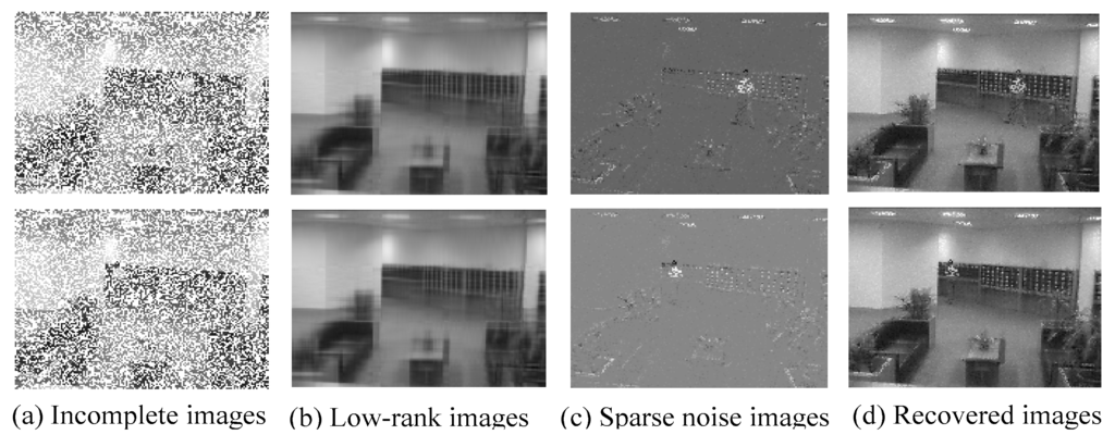
Figure 7.
Background modeling from lobby video. (a) draws the images with missing entries, (b) plots the recovered background, i.e., the low-rank images, (c) shows the recovered foreground, i.e., the sparse noised images, and (d) displays the recovered images.
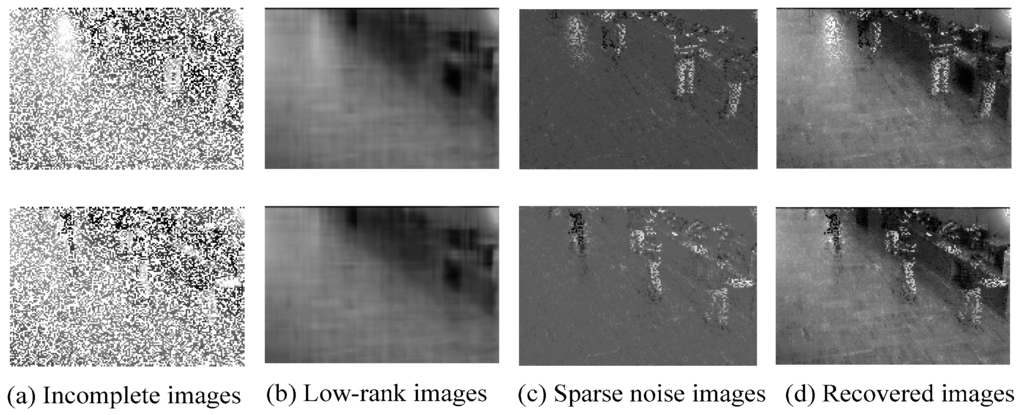
Figure 8.
Background modeling from bootstrap video. (a) draws the images with missing entries, (b) plots the recovered background, i.e., the low-rank images, (c) shows the recovered foreground, i.e., the sparse noised images, and (d) diplays the recovered images.
To evaluate the completion performance of GLRTR, we define the Relative Approximate Error (RAE) as , where is the original video tensor without Gaussian noise corruptions and missing entries, and is the approximated term of . The RAE of the Lobby dataset is 8.94% and that of the Bootstrap dataset is 20.11%. These results demonstrate GLRTR can complete approximately the missing entries to a certain degree. There are two reasons for that the Bootstrap dataset has relatively large RAE: one is its more complex foreground and the other is that the entries of the foreground can not be recovered when they are missing. In summary, GLRTR is robust to gross corruption, Gaussian noise and missing values.
7. Conclusions
In this paper, we investigate a generalized model of LRTR in which large sparse corruption, missing entries and Gaussian noise are taken into account. For the generalized LRTR, we establish an optimization problem that minimizes the weighted combination of the tensor nuclear norm, the l1 norm and the Frobenius norm. To address this minimization problem, we present an iterative scheme based on the technique of ADMM. The experimental results on synthetic data and real-world video datasets illustrate that the proposed method is efficient and feasible in recovering the low-rank components and completing missing entries. In the future, we will consider the theoretical conditions for exact recoverability and other scalable algorithms.
Acknowledgments
This work is partially supported by the National Natural Science Foundation of China (No. 61403298, No. 11526161 and No. 11401357), and the Natural Science Basic Research Plan in Shaanxi Province of China (No. 2014JQ8323).
Author Contributions
Jiarong Shi constructed the model, developed the algorithm and wrote the manuscript. Qingyan Yin designed the experiments. Xiuyun Zheng and Wei Yang implemented all experiments. All four authors were involved in organizing and refining the manuscript. All authors have read and approved the final manuscript.
Conflicts of Interest
The authors declare no conflicts of interest.
References
- Candès, E.J.; Recht, B. Exact matrix completion via convex optimization. Found. Comput. Math. 2009, 9, 717–772. [Google Scholar] [CrossRef]
- Candès, E.J.; Li, X.; Ma, Y.; Wright, J. Robust principal component analysis? J. ACM. 2011, 58, 37. [Google Scholar] [CrossRef]
- Liu, G.; Lin, Z.; Yan, S.; Sun, J.; Yu, Y.; Ma, Y. Robust recovery of subspace structures by low-rank representation. IEEE Trans. Pattern Anal. Mach. Intell. 2013, 35, 171–184. [Google Scholar] [CrossRef] [PubMed]
- Candès, E.J.; Plan, Y. Matrix completion with noise. P. IEEE. 2010, 98, 925–936. [Google Scholar] [CrossRef]
- Zhou, Z.; Li, X.; Wright, J.; Candès, E.J.; Ma, Y. Stable principal component pursuit. In Proceedings of the 2010 IEEE International Symposium on Information Theory Proceedings (ISIT), Austin, TX, USA, 13–18 June 2010.
- Xu, H.; Caramanis, C.; Sanghavi, S. Robust PCA via outlier pursuit. IEEE Trans. Inf. Theory. 2012, 58, 3047–3064. [Google Scholar] [CrossRef]
- Shi, J.; Zheng, X.; Yong, L. Incomplete robust principal component analysis. ICIC Express Letters, Part B Appl. 2014, 5, 1531–1538. [Google Scholar]
- Shi, J.; Yang, W.; Yong, L.; Zheng, X. Low-rank representation for incomplete data. Math. Probl. Eng. 2014, 10. [Google Scholar] [CrossRef]
- Liu, Y.; Jiao, L.C.; Shang, F.; Yin, F.; Liu, F. An efficient matrix bi-factorization alternative optimization method for low-rank matrix recovery and completion. Neural Netw. 2013, 48, 8–18. [Google Scholar] [CrossRef] [PubMed]
- Liu, Y.; Jiao, L.C.; Shang, F. A fast tri-factorization method for low-rank matrix recovery and completion. Pattern Recogn. 2013, 46, 163–173. [Google Scholar] [CrossRef]
- De Lathauwer, L.; Castaing, J. Tensor-based techniques for the blind separation of DS–CDMA signals. Signal Process. 2007, 87, 322–336. [Google Scholar] [CrossRef]
- Kolda, T.G.; Bader, B.W. Tensor decompositions and applications. SIAM Rev. 2009, 51, 455–500. [Google Scholar] [CrossRef]
- Liu, J.; Musialski, P.; Wonka, P.; Ye, J. Tensor completion for estimating missing values in visual data. IEEE Trans. Patt. Anal. Mach. Intel. 2013, 35, 208–220. [Google Scholar] [CrossRef] [PubMed]
- Shi, J.; Zhou, S.; Zheng, X. Multilinear robust principal component analysis. Acta Electronica Sinica. 2014, 42, 1480–1486. [Google Scholar]
- Tomasi, G.; Bro, R. PARAFAC and missing values. Chemom. Intell. Lab. Syst. 2005, 75, 163–180. [Google Scholar] [CrossRef]
- Shi, J.; Jiao, L.C.; Shang, F. Tensor completion algorithm and its applications in face recognition. Pattern Recognit. Artif. Intell. 2011, 24, 255–261. [Google Scholar]
- Kressner, D.; Steinlechner, M.; Vandereycken, B. Low-rank tensor completion by Riemannian optimization. BIT Numer. Math. 2014, 54, 447–468. [Google Scholar] [CrossRef]
- Shi, J.; Yang, W.; Yong, L.; Zheng, X. Low-rank tensor completion via Tucker decompositions. J. Comput. Inf. Syst. 2015, 11, 3759–3768. [Google Scholar]
- Gandy, S.; Recht, B.; Yamada, I. Tensor completion and low-n-rank tensor recovery via convex optimization. Inv. Probl. 2011, 27, 19. [Google Scholar] [CrossRef]
- Liu, Y.; Shang, F. An efficient matrix factorization method for tensor completion. IEEE Signal Process. Lett. 2013, 20, 307–310. [Google Scholar] [CrossRef]
- Tan, H.; Cheng, B.; Wang, W.; Zhang, Y.J.; Ran, B. Tensor completion via a multi-linear low-n-rank factorization model. Neurocomputing. 2014, 133, 161–169. [Google Scholar] [CrossRef]
- Goldfarb, D.; Qin, Z. Robust low-rank tensor recovery: Models and algorithms. SIAM J. Matrix Anal. Appl. 2014, 35, 225–253. [Google Scholar] [CrossRef]
- Cai, J.F.; Candès, E.J.; Shen, Z. A singular value thresholding algorithm for matrix completion. SIAM J. Optimiz. 2010, 20, 1956–1982. [Google Scholar] [CrossRef]
- Boyd, S.; Parikh, N.; Chu, E.; Peleato, B.; Eckstein, J. Distributed optimization and statistical learning via the alternating direction method of multipliers. Found. Trends Mach. Learn. 2011, 3, 1–122. [Google Scholar] [CrossRef]
- Rockafellar, R.T. Monotone operators and the proximal point algorithm. SIAM J. Control Optim. 1976, 14, 877–898. [Google Scholar] [CrossRef]
- Databases of Lobby and Bootstrap. Available online: http://perception.i2r.a-star.edu.sg/bk_ model/bk_index.html (accessed on 1 November 2015).
© 2016 by the authors; licensee MDPI, Basel, Switzerland. This article is an open access article distributed under the terms and conditions of the Creative Commons Attribution (CC-BY) license (http://creativecommons.org/licenses/by/4.0/).