1. Introduction
The problem of finding a simple zero of a nonlinear equation
is an often discussed problem in many applications of science and technology. The most commonly used method is the Newton-Raphson method (simply called as Newton’s method). Many higher order variants of Newton’s method have been developed and rediscovered in the last 15 years. Recently, the order of convergence of many variants of Newton’s method has been improved using the same number of functional evaluations by means of weight functions (see [
1,
2,
3,
4,
5,
6] and the references therein). The aim of such research is to develop optimal methods which satisfy Kung-Traub’s conjecture. In this paper, we develop 2-point methods with 1 function and 2 first derivative evaluations for solving quadratic equations and study Kung-Traub’s conjecture for these methods. We extend these methods to systems of quadratic equations and conduct some numerical experiments to test the efficiencies of the methods.
2. Developments of the Methods
Let define an Iterative Function (I.F.).
Definition 1. [7] If the sequence tends to a limit in such a way thatfor , then the order of convergence of the sequence is said to be p, and C is known as the asymptotic error constant. If ,
or , the convergence is said to be linear, quadratic or cubic, respectively. Let , then the relationis called the error equation. The value of p is called the order of convergence of the method. Definition 2. [8] The Efficiency Index is given bywhere d is the total number of new function evaluations (the values of f and its derivatives) per iteration. Let be determined by new information at
No old information is reused. Thus,
Then
ψ is called a multipoint I.F without memory.
Kung-Traub’s Conjecture [
9]
Let
ψ be an I.F. without memory with
d evaluations. Then
where
is the maximum order.
The second order Newton I.F. (2
ndNR) is given by
The 2
ndNR I.F. is a 1-point I.F. with 2 functions evaluations and it satisfies the Kung-Traub conjecture with
. Thus,
. The 2-point fourth order Jarratt I.F. (4
thJM) [
10] is given by
The 4thJM I.F. with 3 function evaluations satisfies the Kung-Traub conjecture with .
According to Kung-Traub’s conjecture, it is not possible to obtain an I.F. with three function evaluations reaching an order greater than four. We show that this conjecture fails for quadratic functions.
We consider the quadratic function
, where
are constants. Consider the following I.F. for quadratic function:
where
where
’s are constants.
The error equation of the I.F. defined by Equation (
7) for
is given by
where
.
Eliminating the terms in
,
we obtain a system of 6 linear equations with 6 unknowns:
where
whose solutions are given by
We note that is a lower triangular matrix and the solutions are easily obtained once the first solution is obtained from the first equation.
In this way, we obtain a family of higher order I.F.s which we term as higher order 2-point Babajee’s Quadratic Iterative Methods for solving quadratic equations (thBQIM).
The first six members of
thBQIM’s family in Equation (
7) with their error equation are
: 2-point 3
rdBQIM I.F.
: 2-point 4
thBQIM I.F.
: 2-point 5
thBQIM I.F.
: 2-point 6
thBQIM I.F.
: 2-point 7
thBQIM I.F.
: 2-point 8
thBQIM I.F.
We note that the maximum order reached by optimal methods with four function evaluations is eight. We have obtained an eighth order 2-point method with only three function evaluations for solving quadratic equations. This implies that the Kung-Traub conjecture fails for quadratic equations.
3. Convergence Analysis
Theorem 3. Let a sufficiently smooth function has a simple root in the open interval D. Then the six members of 2-pointthBQIM
’s family in Equation (
7)
() are of local 3rd to 8th order convergence, respectively. Proof. We will prove the 3rd order convergence of the 2-point 3rdBQIM I.F. and 8th order convergence of the 2-point 8thBQIM I.F.
The proofs for the 2-point 4th to 7th order I.F.s follow on similar lines.
It is easy to see that for a quadratic function,
and
By Taylor expansion and using computer algebra software as Maple
so that
Using Equations (
8) and (
10), we have
which leads to the error equation for the 2-point 3
rdBQIM I.F.
Using Equations (
8) and (
11), we have
which leads to the error equation for the 2-point 8
thBQIM I.F.
☐
We next prove the local convergence of the 2-point thBQIM’s family for any r.
Theorem 4. Let a sufficiently smooth function has a simple root in the open interval D. Then the members of 2-pointthBQIM
’s family in Equation (
7)
are of local th order convergence. Proof. We prove this result by induction.
The case corresponds to the 3rdBQIM I.F.
Assume the 2-point
thBQIM family has order of convergence of
. Then it satisfies the error equation
where
is the asymptotic error constant.
Assume that Equation (
12) holds for
.
Now from Equation (
9), we have
so that
For the case
,
which shows that the 2-point
thBQIM family has
th order of convergence if we choose
☐
From Equation (
14), we can obtain higher order I.F. if we know the asymptotic error constant of the previous I.F.
For example, for the 2-point 3
rdBQIM I.F.,
and from Equation (
14),
and we can obtain the 4
thBQIM I.F.
Similarly, for the 2-point 8
thBQIM I.F.,
and from Equation (
14),
and we can obtain the 2-point 9
thBQIM I.F. with
From Theorem 4, we conclude that we can have a family of order , with only 3 function evaluations.
The Efficiency Index of the 2-point
thBQIM family is given by
In the following section, we extend our methods to systems of equations.
4. Extension to Systems of Equations
Consider the system of nonlinear equations
where
,
,
defined as
and
is a smooth map and
is an open and convex set, where we assume that
is a zero of the system and
is an initial guess sufficiently close to
.
We define the 2-point
thBQIM’s family for systems of quadratic equations as:
where
Using the notations in [
11], it is noted that
.
The error at the th iteration is , where is a p-linear function , is called the error equation and p is the order of convergence.
Observe that is .
The first six members of
thBQIM’s family in Equation (
16) with their error equation are
: 2-point 3
rdBQIM I.F.
: 2-point 4
thBQIM I.F.
: 2-point 5
thBQIM I.F.
: 2-point 6
thBQIM I.F.
: 2-point 7
thBQIM I.F.
: 2-point 8
thBQIM I.F.
4.1. Convergence Analysis
Theorem 5. Let be twice Frechet differentiable at each point of an open convex neighborhood of , that is a solution of the quadratic system . Let us suppose that is continuous and nonsingular in , and is close enough to . Then the sequence obtained using the iterative expressions Equation (16), converge to with order 3 to 8, respectively. Proof. We will prove for the case
. The other cases follow along similar lines. Since
is a quadratic function of several variables, we have
and
Using Equations (
17) and (
19), we have
and the expression for
is given by
The Taylor expansion of Jacobian matrix
is then given by
Therefore, using Equation (
19), we obtain
so that
Using Equations (
20) and (
21), we have, after simplifications,
and, thus,
☐
Theorem 6. Let be twice Frechet differentiable at each point of an open convex neighborhood of , that is a solution of the quadratic system . Let us suppose that is continuous and nonsingular in , and is close enough to . Then the sequence obtained using the iterative expressions Equation (16), converges to with order with the error equation The proof is by induction and follows along similar lines.
Similarly as in the case of scalar equations, we can obtain higher order I.F. for systems if we know the asymptotic error constant of the previous I.F. using
5. Numerical Experiments
5.1. Scalar Equation
We consider the Test problem 1 (TP1) of finding the positive zero of the quadratic function to compare the efficiency of the proposed methods. Numerical computations have been carried out in the MATLAB software rounding to 1000 significant digits. Depending on the precision of the computer, we use the stopping criteria for the iterative process where . Let N be the number of iterations required for convergence. For simplicity, we denote .
The computational order of convergence is given by
We choose
. The results in
Table 1 show that, as the order of the
thBQIM I.F. (r = 1,2,3,4,5,6), the methods converge in less iterations. The computational order of convergence agree with the theoretical order of convergence confirming that Kung-Traub’s conjecture fails for quadratic functions.
Table 1.
Results of the quadratic function for the 3rdBQIM, 4thBQIM, 5thBQIM, 6thBQIM, 7thBQIM and 8thBQIM I.F.s.
Table 1.
Results of the quadratic function for the 3rdBQIM, 4thBQIM, 5thBQIM, 6thBQIM, 7thBQIM and 8thBQIM I.F.s.
| Error |
3 |
4 |
5 |
6 |
7 |
8 |
|---|
| 5.6e−1 | 5.8e−1 | 5.8e−1 | 5.8e−1 | 5.9e−1 | 5.9e−1 |
| 2.3e−2 | 7.7e−3 | 2.8e−3 | 1.1e−3 | 4.3e-4 | 1.8e−4 |
| 3.0e−6 | 7.5e−10 | 3.6e−14 | 3.5e−19 | 6.9e−25 | 2.9e−31 |
| 7.0e−18 | 6.9e−38 | 1.3e−68 | 4.0e−112 | 1.8e−170 | 1.3e−245 |
| 8.7e−53 | 4.9e−150 | - | - | - | - |
| - | - | - | - | - | - |
| ρ | 3 | 4 | 5 | 6 | 7 | 8 |
5.2. Dynamic Behaviour in the Complex Plane
Consider our Test problem 2 (TP2) based on the quadratic function where z is a complex number. We let and which are the roots of unity for . We study the dynamic behaviour of higher order thBQIM I.F.s (). We take a square of points and we apply our iterative methods starting in every in the square. If the sequence generated by the iterative method attempts a zero of the polynomial with a tolerance and a maximum of 100 iterations, we decide that is in the basin of attraction of this zero.
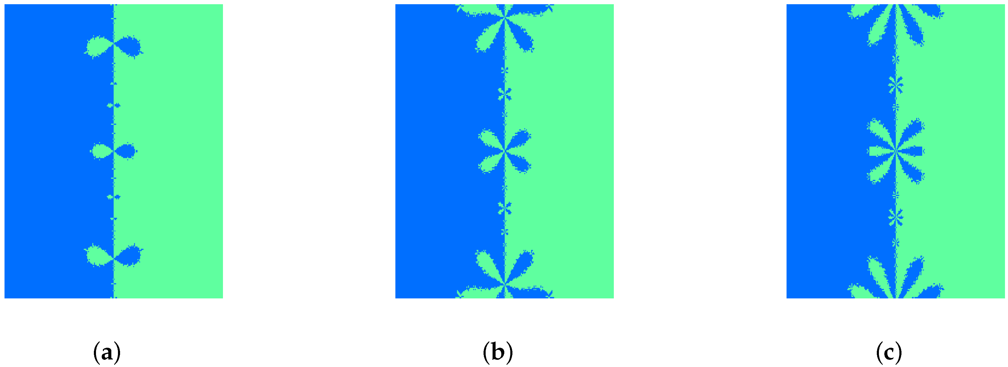
If the iterative method starting in reaches a zero in N iterations (), then we mark this point with a blue color if or green color if . If we conclude that the starting point has diverged and we assign a dark blue color. Let be number of diverging points and we count the number of starting points which converge in 1, 2, 3, 4, 5 or above 5 iterations.
Table 2 shows that all 6 methods are globally convergent and as the order of the method increases, the number of starting points converging to a root in 1 or 2 iterations increases. This is the advantage of higher order methods.
Table 2.
Results of the quadratic function for the 3rdBQIM, 4thBQIM, 5thBQIM, 6thBQIM, 7thBQIM and 8thBQIM I.F.s.
Table 2.
Results of the quadratic function for the 3rdBQIM, 4thBQIM, 5thBQIM, 6thBQIM, 7thBQIM and 8thBQIM I.F.s.
| I.F. | | | | | | | |
|---|
|
3rdBQIM | 56 | 6536 | 28,736 | 16,240 | 5428 | 8540 | 0 |
|
4thBQIM | 232 | 16,908 | 27,532 | 7780 | 3700 | 9564 | 0 |
|
5thBQIM | 528 | 23,348 | 23,196 | 5928 | 3340 | 9196 | 0 |
|
6thBQIM | 928 | 27,880 | 19,680 | 5272 | 3072 | 8704 | 0 |
|
7thBQIM | 1392 | 31,304 | 16,736 | 4856 | 2864 | 8394 | 0 |
|
8thBQIM | 1892 | 33,924 | 14,220 | 4564 | 2788 | 8184 | 0 |
Figure 1.
Polynomiographs of 3rdBQIM, 4thBQIM and 5thBQIM I.F.s. for . (a) 3rdBQIM; (b) 4thBQIM; (c) 5thBQIM.
Figure 1.
Polynomiographs of 3rdBQIM, 4thBQIM and 5thBQIM I.F.s. for . (a) 3rdBQIM; (b) 4thBQIM; (c) 5thBQIM.
Bahman Kalantari coined the term “polynomiography” to be the art and science of visualization in the approximation of roots of polynomial using I.F. [
12].
Figure 1 and
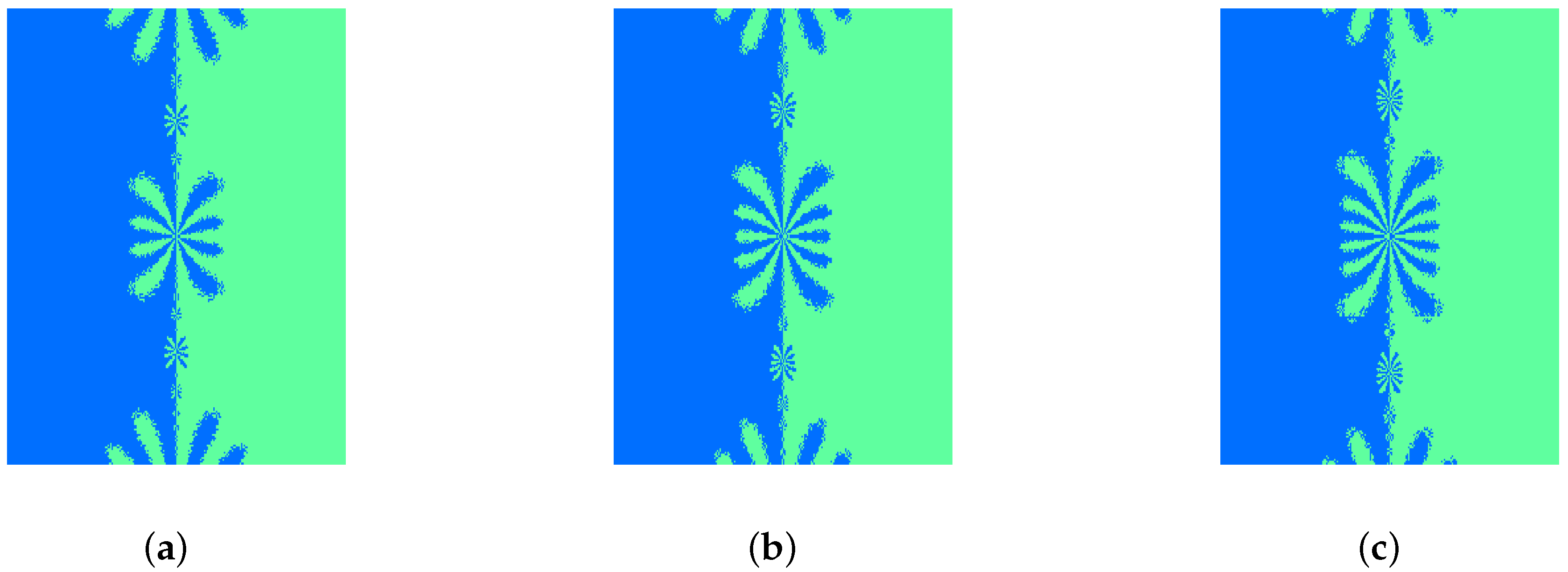
Figure 2 show the polynomiography of the six methods. It can be observed as the order of the method increases, the methods behave more chaotically (the size of the “petals” become larger).
Figure 2.
Polynomiographs of 6thBQIM, 7thBQIM and 8thBQIM I.F.s. for . (a) 6thBQIM; (b) 7thBQIM; (c) 8thBQIM.
Figure 2.
Polynomiographs of 6thBQIM, 7thBQIM and 8thBQIM I.F.s. for . (a) 6thBQIM; (b) 7thBQIM; (c) 8thBQIM.
5.3. Systems of Quadratic Equations
For our numerical experiments in this section, the approximate solutions are calculated correct to 1000 digits by using variable precision arithmetic in MATLAB. We use the following stopping criterion for the numerical scheme:
For a system of equations, we used the approximated computational order of convergence
given by (see [
13])
We consider the
Test Problem 3 (TP3) which is a system of 2 equations:
Using the substitution method, Equation (
25) reduces to the quadratic equation
whose positive root is given by
Therefore
We use
as starting vector and apply our Equation (
16),
to calculate the approximate solutions of Equation (
25).
Table 3.
Results of the TP3 for the 3rdBQIM, 4thBQIM, 5thBQIM, 6thBQIM, 7thBQIM and 8thBQIM I.F.s.
Table 3.
Results of the TP3 for the 3rdBQIM, 4thBQIM, 5thBQIM, 6thBQIM, 7thBQIM and 8thBQIM I.F.s.
| Error |
3 |
4 |
5 |
6 |
7 |
8 |
|---|
| 4.2e−1 | 4.3e−1 | 4.3e−1 | 4.3e−1 | 4.3e−1 | 4.3e−1 |
| 9.2e−3 | 2.5e−3 | 7.6e−4 | 2.5e−4 | 8.6e−5 | 3.1e−5 |
| 6.0e−8 | 1.4e−12 | 5.1e−18 | 2.9e−24 | 2.7e−31 | 4.0e−39 |
| 1.6e−23 | 1.5e−49 | 7.5e−89 | 7.4e−144 | 7.0e−217 | 3.0e−310 |
| 3.4e−70 | 1.9e−197 | - | - | - | - |
| 3 | 4 | 5 | 6 | 7 | 8 |
Table 3 shows that as the order of the methods increase the methods converge in less iterations (4 iterations) and with a smaller error. Similarly, as in the case for scalar equations, the computational order of convergence for this system of 2 equations agree with the theoretical one.
We next consider the
Test Problem 4 (TP4) [
14]
Using the elimination method, Equation (
26) reduces to the simple quadratic equation
whose positive root is given by
and therefore
.
Using
as starting vector far from the root, we apply our methods (
16),
to find the numerical solutions of Equation (
26).
Table 4.
Results of TP4 for the 3rdBQIM, 4thBQIM, 5thBQIM, 6thBQIM, 7thBQIM and 8thBQIM I.F.s.
Table 4.
Results of TP4 for the 3rdBQIM, 4thBQIM, 5thBQIM, 6thBQIM, 7thBQIM and 8thBQIM I.F.s.
| Error |
3 |
4 |
5 |
6 |
7 |
8 |
|---|
| 2.0e0 | 2.2e0 | 2.3e0 | 2.4e0 | 2.4e0 | 2.5e0 |
| 5.3e−1 | 3.8e−1 | 2.8e−1 | 2.2e−1 | 1.7e−1 | 1.4e−1 |
| 3.5e−2 | 5.0e−3 | 6.3e−4 | 6.8e−5 | 6.2e−6 | 4.5e−7 |
| 3.1e−5 | 1.5e−9 | 9.2e−16 | 3.5e−24 | 4.1e−35 | 6.9e−49 |
| 5.2e−14 | 2.3e−35 | 9.0e−75 | 8.3e−140 | 2.5e−239 | 0 |
| 2.7e−40 | 1.3e−138 | - | - | - | - |
| 4.2e−119 | - | - | - | - | - |
| 3.00 | 4.00 | 4.98 | 6.00 | 7.00 | 7.63 |
In
Table 4, with the starting vector distant from the root, we observe that the methods take more iterations to converge. As from the third iteration, the iterate of the methods are close to the root and they converge to the root at their respective rate of convergence.
We next consider the
Test Problem 5 (TP5) which is a system of 4 equations [
15].
Using the substitution method, Equation (
27) reduces to the simple quadratic equation
whose positive root is given by
Therefore
and
Using
as starting vector, we apply our Equation (
16),
to find the numerical solutions of Equation (
27).
In
Table 5, we deduce that similar observations on computational order of convergence can be made for this system of four equations.
Table 5.
Results of TP5 for the 3rdBQIM, 4thBQIM, 5thBQIM, 6thBQIM, 7thBQIM and 8thBQIM I.F.s.
Table 5.
Results of TP5 for the 3rdBQIM, 4thBQIM, 5thBQIM, 6thBQIM, 7thBQIM and 8thBQIM I.F.s.
| Error |
3 |
4 |
5 |
6 |
7 |
8 |
|---|
| 1.4e−1 | 1.4e−1 | 1.4e−1 | 1.4e−1 | 1.4e−1 | 1.4e−1 |
| 1.7e−3 | 3.5e−4 | 8.1e−5 | 2.0e−5 | 5.2e−6 | 1.4e−6 |
| 2.4e−9 | 8.6e−15 | 2.6e−21 | 7.1e−29 | 1.7e−37 | 3.9e−47 |
| 6.5e−27 | 3.1e−57 | 9.7e−104 | 1.4e−169 | 7.9e−258 | 0 |
| 1.3e−79 | - | - | - | - | - |
| 3 | 4 | 5 | 6 | 7 | 8.1 |
5.4. Application
As an application, we consider the quadratic integral equation of the type:
Equation (
28) appears in [
16] and is known as Chandrasekhar’s integral equation. It arises from the study of the radiative transfer theory, the transport of neutrons and the kinetic theory of the gases. It is studied in [
17] and, under certain conditions for the kernel, in [
18,
19].
We define the kernel
as a continuous function in
such that
and
. Moreover, we assume that
is a given function and
λ is a real constant. The solution of Equation (
28) is equivalent to solving the equation
, where
and
We choose
and
so that we are required to solve the following equation:
If we discretize the integral given in Equation (
29) using the Mid-point Integration Rule with
n grid points
we obtain the resulting system of non-linear equations:
The λ are equally spaced with in the interval . We choose and as the starting vector. In this case, for each λ, we let be the minimum number of iterations for which the infinity norm between the successive approximations , where the approximation is calculated correct to 16 digits (double precision in MATLAB). Let be the mean of iteration number for the 49 λ’s.
All methods converge for all 49 values of
λ. The results are given in
Table 6 which shows that all methods converge in less than five iterations. It is the 8
thBQIM I.F. which has the greatest number of
λ converging in two or three iterations and the smallest mean iteration number. We also observe that there is a small difference in the mean iteration number between the 7
thBQIM and 8
thBQIM I.F.s. Developing 9th or higher order I.F.s would not be necessary for this application.
Table 6.
Results of the Chandrasekhar’s integral equation for the 3rdBQIM, 4thBQIM, 5thBQIM, 6thBQIM, 7thBQIM and 8thBQIM I.F.s.
Table 6.
Results of the Chandrasekhar’s integral equation for the 3rdBQIM, 4thBQIM, 5thBQIM, 6thBQIM, 7thBQIM and 8thBQIM I.F.s.
| Method | | | | | | |
|---|
|
3rdBQIM | 0 | 21 | 23 | 5 | 0 | 3.67 |
|
4thBQIM | 1 | 34 | 13 | 1 | 0 | 3.29 |
|
5thBQIM | 3 | 38 | 8 | 0 | 0 | 3.10 |
|
6thBQIM | 3 | 40 | 6 | 0 | 0 | 3.06 |
|
7thBQIM | 3 | 41 | 5 | 0 | 0 | 3.04 |
|
8thBQIM | 3 | 42 | 4 | 0 | 0 | 3.02 |
6. Conclusions and Future Work
In this work, we have shown that Kung-Traub’s conjecture fails for quadratic functions, that is, we can obtain iterative methods for solving quadratic equations with three functions evaluations reaching order of convergence greater than four. Furthermore, using weight functions, we showed that it is possible to develop methods with three function evaluations of any order. These methods are extended to systems involving quadratic equations. We have developed 3rd to 8th order methods and applied them in some numerical experiments including an application to Chandrasekhar’s integral equation. The dynamic behaviour of the methods were also studied. This research will open
the door to new avenues. For example, for solving quadratic equations numerically, we can improve the order of fourth order method with two function and one first derivative evaluations (Ostrowski’s method [
8]) or fourth order derivative-free method with three function evaluations (higher order Steffensen’s method (see [
20])). The question we now pose: Is it possible to develop fifth order methods with three function evaluations for solving cubic or higher order polynomials? This is for future considerations.


