On Some Improved Harmonic Mean Newton-Like Methods for Solving Systems of Nonlinear Equations

Abstract

In this work, we have developed a fourth order Newton-like method based on harmonic mean and its multi-step version for solving system of nonlinear equations. The new fourth order method requires evaluation of one function and two first order Fréchet derivatives for each iteration. The multi-step version requires one more function evaluation for each iteration. The proposed new scheme does not require the evaluation of second or higher order Fréchet derivatives and still reaches fourth order convergence. The multi-step version converges with order $2r+4$, where r is a positive integer and $r\ge 1$. We have proved that the root α is a point of attraction for a general iterative function, whereas the proposed new schemes also satisfy this result. Numerical experiments including an application to 1-D Bratu problem are given to illustrate the efficiency of the new methods. Also, the new methods are compared with some existing methods.

1. Introduction

An often discussed problem in many applications of science and technology is to find a real zero of a system of nonlinear equations $F\left(x\right)=0$, where $F\left(x\right)={(f_1\left(x\right),f_2\left(x\right),...,f_n\left(x\right))}^T$, $x={(x_1,x_2,...,x_n)}^T$, $f_i:{\mathbb{R}}^n\to \mathbb{R},\forall i=1,2,\dots ,n$ and $F:D\subset {\mathbb{R}}^n\to {\mathbb{R}}^n$ is a smooth map and D is an open and convex set, where we assume that $\alpha ={({\alpha }_1,{\alpha }_2,...,{\alpha }_n)}^T$ is a zero of the system and $x^{\left(0\right)}={\left(x_1^{\left(0\right)},x_2^{\left(0\right)},...,x_n^{\left(0\right)}\right)}^T$ is an initial guess sufficiently close to α. For example, problems of the above type arise while solving boundary value problems for differential equations. The differential equations are reduced to system of nonlinear equations, which are in turn solved by the familiar Newton’s iteration method having convergence order two [1]. The Newton method (2^ndNM) is given by

$$x^{(k+1)}=G_{2^{nd}NM}\left(x^{\left(k\right)}\right)=x^{\left(k\right)}-u\left(x^{\left(k\right)}\right),u\left(x^{\left(k\right)}\right)={\left[F^{\prime }\left(x^{\left(k\right)}\right)\right]}^{-1}F\left(x^{\left(k\right)}\right)$$

(1)

Homeier [2] has proposed a third order iterative method called Harmonic Mean Newton’s method for solving a single nonlinear equation. Analogous to this method [2], we consider the following extension to solve a system of nonlinear equation $F\left(x\right)=0$, henceforth called as $3^{rd}HM$:

$$x^{(k+1)}=G_{3^{rd}HM}\left(x^{\left(k\right)}\right)=x^{\left(k\right)}-\frac{1}{2}\left({\left[F^{\prime }\left(x^{\left(k\right)}\right)\right]}^{-1}+{\left[F^{\prime }(x^{\left(k\right)}-u\left(x^{\left(k\right)}\right))\right]}^{-1}\right)F\left(x^{\left(k\right)}\right)$$

(2)

We note that ${\displaystyle \frac{1}{2}\left({\left[F^{\prime }\left(x^{\left(k\right)}\right)\right]}^{-1}+{\left[F^{\prime }(x^{\left(k\right)}-u\left(x^{\left(k\right)}\right))\right]}^{-1}\right)}$ is the average of the inverses of two Jacobians. In general, such third order methods free of second derivatives like Equation (2) can be used for solving system of nonlinear equations. These methods require one function evaluation and two first order Fréchet derivative evaluations. The convergence analysis of a few such methods using point of attraction theory can be found in [3]. This $3^{rd}HM$ method is more efficient than Halley’s method because it does not require the evaluation of a third order tensor of $n^3$ values while finding the number of function evaluations.

Furthermore, the $3^{rd}HM$ methods are less efficient than two-step fourth order Newton’s method ($4^{th}NR$)

$$x^{(k+1)}=G_{4^{th}NR}\left(x^{\left(k\right)}\right)=G_{2^{nd}NM}\left(x^{\left(k\right)}\right)-F^{\prime }{\left(G_{2^{nd}NM}\left(x^{\left(k\right)}\right)\right)}^{-1}F\left(G_{2^{nd}NM}\left(x^{\left(k\right)}\right)\right)$$

(3)

which was recently rediscovered by Noor et al. [4] using the variational iteration technique. Recently Sharma et al. [5] developed the fourth order method, which is given by

$$\begin{array}{c}{x}^{(k+1)}=G_{4^{th}SGS}\left(x^{\left(k\right)}\right)=x^{\left(k\right)}-W\left(x^{\left(k\right)}\right)u\left(x^{\left(k\right)}\right),\hfill \\ W\left(x^{\left(k\right)}\right)=-\frac{1}{2}I+\frac{9}{8}{\left[F^{\prime }\left(y\left(x^{\left(k\right)}\right)\right)\right]}^{-1}{F}^{\prime }\left(x^{\left(k\right)}\right)+\frac{3}{8}{\left[F^{\prime }\left(x^{\left(k\right)}\right)\right]}^{-1}{F}^{\prime }\left(y\left(x^{\left(k\right)}\right)\right)\hfill \\ y\left(x^{\left(k\right)}\right)=x^{\left(k\right)}-\frac{2}{3}u\left(x^{\left(k\right)}\right)\hfill \end{array}$$

(4)

Cordero et al. [6] presented a sixth order method, which is given by

$$\begin{array}{c}{x}^{(k+1)}=G_{6^{th}CHMT}\left(x^{\left(k\right)}\right)=z\left(x^{\left(k\right)}\right)-{\left[F^{\prime }(x^{\left(k\right)}-u\left(x^{\left(k\right)}\right))\right]}^{-1}F\left(z\left(x^{\left(k\right)}\right)\right)\hfill \\ z\left(x^{\left(k\right)}\right)=x^{\left(k\right)}-u(x^{\left(k\right)}-\left[2I-F^{\prime }{\left(x^{\left(k\right)}\right)}^{-1}{F}^{\prime }(x^{\left(k\right)}-u\left(x^{\left(k\right)}\right))\right]{\left[F^{\prime }\left(x^{\left(k\right)}\right)\right]}^{-1}F(x^{\left(k\right)}-u\left(x^{\left(k\right)}\right))\hfill \end{array}$$

(5)

Recently, an improved fourth order version from a third order method for solving a single nonlinear equation is found in [7]. In the current paper, similar to the method found in [7], a multivariate version having fourth order convergence is proposed. The rest of this paper is organized as follows. In Section 2, we present a new algorithm (optimal) that has fourth order convergence by using only three function evaluations and a multi-step version with order $2r+4$, where r is a positive integer and $r\ge 1$ for solving systems of nonlinear equations. In Section 3, we study the convergence analysis of the new methods using the point of attraction theory. Section 4 presents numerical examples and comparison with some existing methods. Furthermore, we also study an application problem, i.e., the 1-D Bratu problem [8]. A brief conclusion is given in Section 5.

2. Development of the Methods

Babajee [7] has recently improved the $3^{rd}HM$ method to get a fourth order method for single equation

$$\left\{\begin{array}{c}{y}_k=x_k-\frac{2}{3}\frac{f\left(x_k\right)}{f^{\prime }\left(x_k\right)}\hfill \\ x_{k+1}=x_k-\frac{1}{2}\left[\frac{f\left(x_k\right)}{f^{\prime }\left(x_k\right)}+\frac{f\left(x_k\right)}{f^{\prime }\left(y_k\right)}\right]\left[1-\frac{1}{4}\left(\frac{f^{\prime }\left(y_k\right)}{f^{\prime }\left(x_k\right)}-1\right)+\frac{1}{2}{\left(\frac{f^{\prime }\left(y_k\right)}{f^{\prime }\left(x_k\right)}-1\right)}^2\right]\hfill \end{array}\right.$$

This method is one of the member in the family of higher order multi-point iterative methods based on power mean for solving single nonlinear equation by Babajee et al. [9].

We next extend the above idea to the multivariate case. For the method given in Equation (2), we propose an improved fourth order Harmonic Mean Newton’s method ($4^{th}HM$) for solving systems of nonlinear equations as follows:

$$\begin{array}{c}{x}^{(k+1)}=G_{4^{th}HM}\left(x^{\left(k\right)}\right)=x^{\left(k\right)}-H_1\left(x^{\left(k\right)}\right)A\left(x^{\left(k\right)}\right)F\left(x^{\left(k\right)}\right)\hfill \\ H_1\left(x^{\left(k\right)}\right)=I-\frac{1}{4}(\tau \left(x^{\left(k\right)}\right)-I)+\frac{1}{2}{(\tau \left(x^{\left(k\right)}\right)-I)}^2,\tau \left(x^{\left(k\right)}\right)={\left[F^{\prime }\left(x^{\left(k\right)}\right)\right]}^{-1}{F}^{\prime }\left(y\left(x^{\left(k\right)}\right)\right)\hfill \\ A\left(x^{\left(k\right)}\right)=\frac{1}{2}\left({\left[F^{\prime }\left(x^{\left(k\right)}\right)\right]}^{-1}+{\left[F^{\prime }\left(y\left(x^{\left(k\right)}\right)\right)\right]}^{-1}\right),y\left(x^{\left(k\right)}\right)=x^{\left(k\right)}-\frac{2}{3}u\left(x^{\left(k\right)}\right)\hfill \end{array}$$

(6)

where I is the $n\times n$ identity matrix. We further improve the $4^{th}HM$ method by additional function evaluations to get a multi-step version called ${(2r+4)}^{th}$HM method given by

$$\begin{array}{c}{x}^{(k+1)}=G_{{(2r+4)}^{th}HM}\left(x^{\left(k\right)}\right)={\mu }_r\left(x^{\left(k\right)}\right)\hfill \\ {\mu }_j\left(x^{\left(k\right)}\right)={\mu }_{j-1}\left(x^{\left(k\right)}\right)-H_2\left(x^{\left(k\right)}\right)A\left(x^{\left(k\right)}\right)F\left({\mu }_{j-1}\left(x^{\left(k\right)}\right)\right)\hfill \\ H_2\left(x^{\left(k\right)}\right)=2I-\tau \left(x^{\left(k\right)}\right),j=1,2,...,r,r\ge 1\hfill \\ {\mu }_0\left(x^{\left(k\right)}\right)=G_{4^{th}HM}\left(x^{\left(k\right)}\right)\hfill \end{array}$$

(7)

Note that this multi-step version has order $2r+4$, where r is a positive integer and $r\ge 0$. The case $r=0$ is the $4^{th}HM$ method.

3. Convergence Analysis

The main theorem is going to be demonstrated by means of the n-dimensional Taylor expansion of the functions involved. In the following, we use certain notations and results found in [10]:

Let $F:D\subseteq {\mathbb{R}}^n⟶{\mathbb{R}}^n$ be sufficiently Fréchet differentiable in D. Suppose the qth derivative of F at $u\in {\mathbb{R}}^n$, $q\ge 1$, is the q-linear function $F^{\left(q\right)}\left(u\right):{\mathbb{R}}^n\times \cdots \times {\mathbb{R}}^n⟶{\mathbb{R}}^n$ such that $F^{\left(q\right)}\left(u\right)(v_1,\dots ,v_q)\in R^n$. Given $\alpha +h\in {\mathbb{R}}^n$, which lies in a neighborhood of a solution α of the nonlinear system $F\left(x\right)=0$, Taylor’s expansion can be applied (assuming Jacobian matrix $F^{\prime }\left(\alpha \right)$ is nonsingular) to obtain

$$F(\alpha +h)=F^{\prime }\left(\alpha \right)\left[h+\sum _{q=2}^{p-1}{C}_q{h}^q\right]+O\left(h^p\right)$$

(8)

where $C_q=(1/q!){\left[F^{\prime }\left(\alpha \right)\right]}^{-1}{F}^{\left(q\right)}\left(\alpha \right)$, $q\ge 2$. It is noted that $C_q{h}^q\in {\mathbb{R}}^n$ since $F^{\left(q\right)}\left(\alpha \right)\in \mathcal{L}({\mathbb{R}}^n\times \cdots \times {\mathbb{R}}^n,{\mathbb{R}}^n)$ and ${\left[F^{\prime }\left(\alpha \right)\right]}^{-1}\in \mathcal{L}\left({\mathbb{R}}^n\right)$. Also, we can expand $F^{\prime }(\alpha +h)$ in Taylor series

$$F^{\prime }(\alpha +h)=F^{\prime }\left(\alpha \right)\left[I+\sum _{q=2}^{p-1}q{C}_q{h}^{q-1}\right]+O\left(h^p\right)$$

(9)

where I is the identity matrix. It is also noted that $q{C}_q{h}^{q-1}\in \mathcal{L}\left({\mathbb{R}}^n\right)$. Denote $e^{\left(k\right)}=x^{\left(k\right)}-\alpha$, so the error at the $(k+1)$th iteration is $e^{(k+1)}=L{e^{\left(k\right)}}^p+O\left({e^{\left(k\right)}}^{p+1}\right)$, where L is a p-linear function $L\in \mathcal{L}({\mathbb{R}}^n\times \cdots \times {\mathbb{R}}^n,{\mathbb{R}}^n)$ is called the error equation and p is the order of convergence. Observe that ${e^{\left(k\right)}}^p$ is $(e^{\left(k\right)},e^{\left(k\right)},\cdots ,e^{\left(k\right)})$.

In order to prove the convergence order for the Equation (6), we need to recall some important definitions and results from the theory of point of attraction.

Definition (Point of Attraction). [11] Let $G:D\subset {\mathbb{R}}^n\to {\mathbb{R}}^n$. Then α is a point of attraction of the iteration

$$x^{(k+1)}=G\left(x^{\left(k\right)}\right),k=0,1,...$$

(10)

if there is an open neighborhood S of α defined by

$$S\left(\alpha \right)=\{x\in {\mathbb{R}}^n|\parallel x-\alpha \parallel <\delta \},\delta >0,$$

such that $S\subset D$ and, for any $x^{\left(0\right)}\in S$, the iterating $\left\{x^{\left(k\right)}\right\}$ defined by Equation (10) all lie in D and converge to α.

Theorem 1 (Ostrowski Theorem). [11] Assume that $G:D\subset {\mathbb{R}}^n\to {\mathbb{R}}^n$ has a fixed point $\alpha \in int\left(D\right)$ and $G\left(x\right)$ is Fréchet differentiable on α. If

$$\rho \left(G^{\prime }\left(\alpha \right)\right)=\sigma <1$$

(11)

then α is a point of attraction for $x^{(k+1)}=G\left(x^{\left(k\right)}\right)$.

We now prove a general result that shows α is a point of attraction of a general iteration function $G\left(x\right)=P\left(x\right)-Q\left(x\right)R\left(x\right)$.

Theorem 2. Let $F:D\subset {\mathbb{R}}^n⟶{\mathbb{R}}^n$ be sufficiently Fréchet differentiable at each point of an open convex neighborhood D of $\alpha \in D$, which is a solution of the system $F\left(x\right)=0$. Suppose that $P,Q,R:D\subset {\mathbb{R}}^n\to {\mathbb{R}}^n$ are sufficiently Fréchet differentiable functionals (depending on F) at each point in D with $P\left(\alpha \right)=\alpha$, $Q\left(\alpha \right)\ne 0$ and $R\left(\alpha \right)=0$. Then, there exists a ball

$$S=\overline{S}(\alpha ,\delta )=\left\{\parallel \alpha -x\parallel \le \delta \right\}\subset S_0,\delta >0,$$

on which the mapping

$$G:S\to {\mathbb{R}}^n,G\left(x\right)=P\left(x\right)-Q\left(x\right)R\left(x\right),\text{for}\text{all} x\in S$$

is well-defined; moreover, G is Fréchet differentiable at α, thus

$$G^{\prime }\left(\alpha \right)=P^{\prime }\left(\alpha \right)-Q\left(\alpha \right)R^{\prime }\left(\alpha \right).$$

Proof: Clearly, $G\left(\alpha \right)=\alpha$.

$$\begin{array}{c}\parallel G\left(x\right)-G\left(\alpha \right)-G^{\prime }\left(\alpha \right)(x-\alpha )\parallel \hfill \\ =\parallel P\left(x\right)-Q\left(x\right)R\left(x\right)-\alpha -(P^{\prime }\left(\alpha \right)-Q\left(\alpha \right)R^{\prime }\left(\alpha \right))(x-\alpha )\parallel \hfill \\ \le \parallel P\left(x\right)-\alpha -P^{\prime }\left(\alpha \right)(x-\alpha )\parallel +\parallel -Q\left(x\right)R\left(x\right)+Q\left(\alpha \right)R^{\prime }\left(\alpha \right)(x-\alpha )\parallel ,\text{using}\text{triangle}\text{inequality}.\hfill \end{array}$$

Since $P\left(x\right)$ is differentiable in α and $P\left(\alpha \right)=\alpha$, we can assume that δ was chosen sufficiently small such that

$$\parallel P\left(x\right)-\alpha -P^{\prime }\left(\alpha \right)(x-\alpha )\parallel \le ϵ\parallel x-\alpha \parallel ,$$

for all $x\in S$ with $ϵ>0$ depending on δ and $ϵ=0$ in case $P\left(x\right)=x$.

Since P, Q and R are continuously differentiable functions, then $Q^{\prime }$, $R^{\prime }$ and $R^{″}$ are bounded:

$$\parallel Q^{\prime }\left(x\right)\parallel \le K_1,\parallel R^{\prime }\left(x\right)\parallel \le K_2,\parallel R^{\prime \prime }\left(x\right)\parallel \le K_3.$$

Now by mean value theorem for integrals

$$Q\left(x\right)=Q\left(\alpha \right)+{\int }_0^1{Q}^{\prime }(\alpha +t(x-\alpha ))dt(x-\alpha )$$

and

$$R\left(x\right)={\int }_0^1{R}^{\prime }(\alpha +s(x-\alpha ))ds(x-\alpha ),$$

so that

$$\begin{array}{c}\parallel Q\left(x\right)R\left(x\right)-Q\left(\alpha \right)R^{\prime }\left(\alpha \right)(x-\alpha )\parallel \hfill \\ =\parallel Q\left(\alpha \right)\left({\int }_0^1{R}^{\prime }(\alpha +s(x-\alpha ))-R^{\prime }\left(\alpha \right)ds\right){(x-\alpha )}^2\hfill \\ +{\int }_0^1{\int }_0^1{Q}^{\prime }(\alpha +t(x-\alpha ))R^{\prime }(\alpha +s(x-\alpha ))dtds{(x-\alpha )}^2\parallel \hfill \\ \le \parallel Q\left(\alpha \right)\left({\int }_0^1{\int }_0^1{R}^{\prime \prime }(\alpha +s\lambda (x-\alpha ))dsd\lambda \right)s{(x-\alpha )}^2\hfill \\ +{\int }_0^1{\int }_0^1{Q}^{\prime }(\alpha +t(x-\alpha ))R^{\prime }(\alpha +s(x-\alpha ))dtds{(x-\alpha )}^2\parallel ,\text{using}\text{triangle}\text{inequality},\hfill \end{array}$$

$$\begin{array}{c}\le \parallel Q\left(\alpha \right)\parallel {\int }_0^1{\int }_0^1\parallel R^{″}{(\alpha +s\lambda (x-\alpha ))\parallel dsd\lambda \left|s\right|\parallel x-\alpha \parallel }^2\hfill \\ +{\int }_0^1{\int }_0^1\parallel Q^{\prime }(\alpha +t(x-\alpha ))\parallel \parallel R^{\prime }{(\alpha +s(x-\alpha ))\parallel dtds\parallel x-\alpha \parallel }^2,\text{using}\text{Schwartz}\text{inequality},\hfill \\ \le \left(\frac{K_3}{2}\parallel Q\left(\alpha \right)\parallel +K_1{K}_2\right){\parallel x-\alpha \parallel }^2,\text{since}{Q}^{\prime },R^{\prime }\text{and}{R}^{″}\text{are}\text{bounded},\hfill \\ \le \delta \left(\frac{K_3}{2}\parallel Q\left(\alpha \right)\parallel +K_1{K}_2\right)\parallel x-\alpha \parallel ,\text{since}\parallel x-\alpha \parallel \le \delta .\hfill \end{array}$$

Combining, we have

$$\parallel G\left(x\right)-G\left(\alpha \right)-G^{\prime }\left(\alpha \right)(x-\alpha )\parallel \le \delta \left(ϵ+\frac{K_3}{2}\parallel Q\left(\alpha \right)\parallel +K_1{K}_2\right)\parallel x-\alpha \parallel$$

which shows that $G\left(x\right)$ is differentiable in α since δ and ϵ are arbitrary and $\parallel Q\left(\alpha \right)\parallel$, $K_1$, $K_2$ and $K_3$ are constants. Thus $G^{\prime }\left(\alpha \right)=P^{\prime }\left(\alpha \right)-Q\left(\alpha \right)R^{\prime }\left(\alpha \right)$.

Theorem 3. Let $F:D\subseteq {\mathbb{R}}^n⟶{\mathbb{R}}^n$ be sufficiently Fréchet differentiable at each point of an open convex neighborhood D of $\alpha \in {\mathbb{R}}^n$ that is a solution of the system $F\left(x\right)=0$. Let us suppose that $x\in S=\overline{S}(\alpha ,\delta )$ and $F^{\prime }\left(x\right)$ is continuous and nonsingular in α, and $x^{\left(0\right)}$ is close enough to α. Then α is a point of attraction of the sequence $\left\{x^{\left(k\right)}\right\}$ obtained using the iterative expression Equation (6). Furthermore, the sequence converges to α with order 4, where the error equation obtained is

$$e^{(k+1)}=G_{4^{th}HM}\left(x^{\left(k\right)}\right)-\alpha =L_1{e^{\left(k\right)}}^4+O\left({e^{\left(k\right)}}^5\right),L_1=\frac{79}{27}{C}_2^3-\frac{8}{9}{C}_2{C}_3-\frac{1}{9}{C}_3{C}_2+\frac{1}{9}{C}_4$$

(12)

Proof: We first show that α is a point of attraction using Theorem 2. In this case,

$$P\left(x\right)=x,Q\left(x\right)=H_1\left(x\right)A\left(x\right),R\left(x\right)=F\left(x\right).$$

Now, since $F\left(\alpha \right)=0$, we have

$$\begin{array}{c}y\left(\alpha \right)=\alpha -\frac{2}{3}{\left[F^{\prime }\left(\alpha \right)\right]}^{-1}F\left(\alpha \right)=\alpha ,\hfill \\ \tau \left(\alpha \right)=F^{\prime }{\left(\alpha \right)}^{-1}{F}^{\prime }\left(y\left(\alpha \right)\right)={\left[F^{\prime }\left(\alpha \right)\right]}^{-1}{F}^{\prime }\left(y\left(\alpha \right)\right)=I,H_1\left(\alpha \right)=I,\hfill \\ A\left(\alpha \right)=\frac{1}{2}\left({\left[F^{\prime }\left(\alpha \right)\right]}^{-1}+{\left[F^{\prime }\left(y\left(\alpha \right)\right)\right]}^{-1}\right)={\left[F^{\prime }\left(\alpha \right)\right]}^{-1},\hfill \\ Q\left(\alpha \right)=H_1\left(\alpha \right)A\left(\alpha \right)=I{\left[F^{\prime }\left(\alpha \right)\right]}^{-1}={\left[F^{\prime }\left(\alpha \right)\right]}^{-1}\ne 0,\hfill \\ R\left(\alpha \right)=F\left(\alpha \right)=0,R^{\prime }\left(\alpha \right)=F^{\prime }\left(\alpha \right),\hfill \\ P\left(\alpha \right)=\alpha ,P^{\prime }\left(\alpha \right)=I,\hfill \end{array}$$

$$G^{\prime }\left(\alpha \right)=P^{\prime }\left(\alpha \right)-Q\left(\alpha \right)R^{\prime }\left(\alpha \right)=I-{\left[F^{\prime }\left(\alpha \right)\right]}^{-1}{F}^{\prime }\left(\alpha \right)=0,$$

so that $\rho \left(G^{\prime }\left(\alpha \right)\right)=0<1$ and by Ostrowski’s theorem, α is a point of attraction of Equation (6).

We next establish the fourth order convergence of this method. From Equation (8) and Equation (9) we obtain

$$F\left(x^{\left(k\right)}\right)=F^{\prime }\left(\alpha \right)\left[e^{\left(k\right)}+C_2{e^{\left(k\right)}}^2+C_3{e^{\left(k\right)}}^3+C_4{e^{\left(k\right)}}^4\right]+O\left({e^{\left(k\right)}}^5\right)$$

(13)

and

$$F^{\prime }\left(x^{\left(k\right)}\right)=F^{\prime }\left(\alpha \right)\left[I+2C_2{e}^{\left(k\right)}+3C_3{e^{\left(k\right)}}^2+4C_4{e^{\left(k\right)}}^3+5C_5{e^{\left(k\right)}}^4\right]+O\left({e^{\left(k\right)}}^5\right),$$

where $e^{\left(k\right)}=x^{\left(k\right)}-\alpha$.

We have

$${\left[F^{\prime }\left(x^{\left(k\right)}\right)\right]}^{-1}=\left[I+X_1{e}^{\left(k\right)}+X_2{e^{\left(k\right)}}^2+X_3{e^{\left(k\right)}}^3\right]{\left[F^{\prime }\left(\alpha \right)\right]}^{-1}+O\left({e^{\left(k\right)}}^4\right)$$

(14)

where $X_1=-2C_2$, $X_2=4C_2^2-3C_3$ and $X_3=-8C_2^3+6C_2{C}_3+6C_3{C}_2-4C_4$.

Then

$${\left[F^{\prime }\left(x^{\left(k\right)}\right)\right]}^{-1}F\left(x^{\left(k\right)}\right)=e^{\left(k\right)}-C_2{e^{\left(k\right)}}^2+2(C_2^2-C_3){e^{\left(k\right)}}^3+O\left({e^{\left(k\right)}}^4\right),$$

and the expression for $y\left(x^{\left(k\right)}\right)$ is

$$\begin{array}{cc}\hfill y\left(x^{\left(k\right)}\right)=& \alpha +\frac{1}{3}{e}^{\left(k\right)}+\frac{2}{3}{C}_2{e^{\left(k\right)}}^2-\frac{4}{3}(C_2^2-C_3){e^{\left(k\right)}}^3\hfill \\ & +(2C_4-\frac{8}{3}{C}_2{C}_3-2C_3{C}_2+8C_2^3){e^{\left(k\right)}}^4+O\left({e^{\left(k\right)}}^5\right).\hfill \end{array}$$

The Taylor expansion of the Jacobian matrix $F^{\prime }\left(y\left(x^{\left(k\right)}\right)\right)$ is

$$\begin{array}{cc}\hfill F^{\prime }\left(y\left(x^{\left(k\right)}\right)\right)& =F^{\prime }\left(\alpha \right)[I+2C_2(y\left(x^{\left(k\right)}\right)-\alpha )+3C_3{(y\left(x^{\left(k\right)}\right)-\alpha )}^2+4C_4{(y\left(x^{\left(k\right)}\right)-\alpha )}^3\hfill \\ & +5C_5{(y\left(x^{\left(k\right)}\right)-\alpha )}^4]+O\left({e^{\left(k\right)}}^5\right)\hfill \\ & =F^{\prime }\left(\alpha \right)\left[I+N_1{e}^{\left(k\right)}+N_2{e^{\left(k\right)}}^2+N_3{e^{\left(k\right)}}^3\right]+O\left({e^{\left(k\right)}}^4\right),\hfill \\ & N_1=\frac{2}{3}{C}_2,N_2=\frac{4}{3}{C}_2^2+\frac{1}{3}{C}_3,N_3=-\frac{8}{3}{C}_2^3+\frac{8}{3}{C}_2{C}_3+\frac{4}{3}{C}_3{C}_2+\frac{4}{27}{C}_4.\hfill \end{array}$$

Therefore,

$$\begin{array}{cc}\hfill \tau \left(x^{\left(k\right)}\right)& ={\left[F^{\prime }\left(x^{\left(k\right)}\right)\right]}^{-1}{F}^{\prime }\left(y\left(x^{\left(k\right)}\right)\right)\hfill \\ & =I+(N_1+X_1)e^{\left(k\right)}+(N_2+X_1{N}_1+X_2){e^{\left(k\right)}}^2\hfill \\ & +(N_3+X_1{N}_2+X_2{N}_1+X_3){e^{\left(k\right)}}^3+O\left({e^{\left(k\right)}}^4\right)\hfill \\ & =I-\frac{4}{3}{C}_2{e}^{\left(k\right)}+(4C_2^2-\frac{8}{3}{C}_3){e^{\left(k\right)}}^2+\left(-\frac{32}{3}{C}_2^3+8C_2{C}_3+\frac{16}{3}{C}_3{C}_2-\frac{104}{27}{C}_4\right){e^{\left(k\right)}}^3\hfill \\ & +O\left({e^{\left(k\right)}}^4\right)\hfill \end{array}$$

and then

$$\begin{array}{cc}\hfill H_1\left(x^{\left(k\right)}\right)& =I-\frac{1}{4}\left(\tau \left(x^{\left(k\right)}\right)-I\right)+\frac{1}{2}{\left(\tau \left(x^{\left(k\right)}\right)-I\right)}^2\hfill \\ & =I+\frac{1}{3}{C}_2{e}^{\left(k\right)}+\left(-\frac{1}{9}{C}_2^2+\frac{2}{3}{C}_3\right){e^{\left(k\right)}}^2\hfill \\ & +\left(-\frac{8}{3}{C}_2^3+\frac{14}{9}{C}_2{C}_3-\frac{4}{3}{C}_3{C}_2+\frac{26}{27}{C}_4\right){e^{\left(k\right)}}^3+O\left({e^{\left(k\right)}}^4\right)\hfill \end{array}$$

(15)

Also,

$$\begin{array}{c}{\left[F^{\prime }\left(y\left(x^{\left(k\right)}\right)\right)\right]}^{-1}\hfill \\ =\left[I-N_1{e}^{\left(k\right)}+(N_1^2-N_2){e^{\left(k\right)}}^2+\left(N_1{N}_2+N_2{N}_1-N_1^3-N_3\right){e^{\left(k\right)}}^3\right]{\left[F^{\prime }\left(\alpha \right)\right]}^{-1}+O\left({e^{\left(k\right)}}^4\right)\hfill \\ =\left[I+Y_1{e}^{\left(k\right)}+Y_2{e^{\left(k\right)}}^2+Y_3{e^{\left(k\right)}}^3\right]{\left[F^{\prime }\left(\alpha \right)\right]}^{-1}+O\left({e^{\left(k\right)}}^4\right),\hfill \end{array}$$

(16)

where $Y_1=-\frac{2}{3}{C}_2,Y_2=-\frac{8}{9}{C}_2^2-\frac{1}{3}{C}_3,Y_3=\frac{112}{27}{C}_2^3-\frac{22}{9}{C}_2{C}_3-\frac{10}{9}{C}_3{C}_2-\frac{4}{27}{C}_4$

On the other hand, using Equation (14) and Equation (16), the harmonic mean can be expressed as

$$\begin{array}{c}\hfill \begin{array}{cc}\hfill A\left(x^{\left(k\right)}\right)=& [I-\frac{4}{3}{C}_2{e}^{\left(k\right)}+\left(\frac{14}{9}{C}_2^2-\frac{5}{3}{C}_3\right){e^{\left(k\right)}}^2\hfill \\ & +\left(-\frac{52}{27}{C}_2^3+\frac{16}{9}{C}_2{C}_3+\frac{22}{9}{C}_3{C}_2-\frac{56}{27}{C}_4\right){e^{\left(k\right)}}^3]{\left[F^{\prime }\left(\alpha \right)\right]}^{-1}+O\left({e^{\left(k\right)}}^4\right)\hfill \end{array}\end{array}$$

(17)

Using Equation (15) and Equation (17), we have

$$\begin{array}{c}{H}_1\left(x^{\left(k\right)}\right)A\left(x^{\left(k\right)}\right)\hfill \\ =\left[I-C_2{e}^{\left(k\right)}+(C_2^2-C_3){e^{\left(k\right)}}^2+\left(-\frac{106}{27}{C}_2^3+\frac{17}{9}{C}_2{C}_3+\frac{10}{9}{C}_3{C}_2-\frac{10}{9}{C}_4\right){e^{\left(k\right)}}^3\right]{\left[F^{\prime }\left(\alpha \right)\right]}^{-1}\hfill \\ +O\left({e^{\left(k\right)}}^4\right)\hfill \end{array}$$

(18)

Finally, by using Equation (13) and Equation (18) in Equation (6) with some simplifications, the error equation can be expressed as:

$$\begin{array}{cc}\hfill e^{(k+1)}& =x^{\left(k\right)}-\alpha -H_1\left(x^{\left(k\right)}\right)A\left(x^{\left(k\right)}\right)F\left(x^{\left(k\right)}\right)\hfill \\ & =\left(\frac{79}{27}{C}_2^3-\frac{8}{9}{C}_2{C}_3-\frac{1}{9}{C}_3{C}_2+\frac{1}{9}{C}_4\right){e^{\left(k\right)}}^4+O\left({e^{\left(k\right)}}^5\right)\hfill \end{array}$$

(19)

Thus from Equation (19), it can be concluded that the order of convergence of the $4^{th}HM$ method is four.   ☐

For the case $r\ge 1$ we state and prove the following theorem.

Theorem 4. Let $F:D\subseteq {\mathbb{R}}^n⟶{\mathbb{R}}^n$ be sufficiently Fréchet differentiable at each point of an open convex neighborhood D of $\alpha \in {\mathbb{R}}^n$ that is a solution of the system $F\left(x\right)=0$. Let us suppose that $x\in S=\overline{S}(\alpha ,\delta )$ and $F^{\prime }\left(x\right)$ is continuous and nonsingular in α, and $x^{\left(0\right)}$ is close enough to α. Then α is a point of attraction of the sequence $\left\{x^{\left(k\right)}\right\}$ obtained using the iterative expression Equation (7). Furthermore the sequence converges to α with order $2r+4$, wherer is a positive integer and $r\ge 1$.

Proof: In this case,

$$P\left(x\right)={\mu }_{j-1}\left(x\right),Q\left(x\right)=H_2\left(x\right)A\left(x\right),R\left(x\right)=F\left({\mu }_{j-1}\left(x\right)\right),j=1,...,r.$$

We can show by induction that

$${\mu }_{j-1}\left(\alpha \right)=\alpha ,{\mu }_{j-1}^{\prime }\left(\alpha \right)=0,\forall j=1,...,r$$

so that

$$\begin{array}{c}P\left(\alpha \right)={\mu }_{j-1}\left(\alpha \right)=\alpha ,H_2\left(\alpha \right)=I,Q\left(\alpha \right)=H_2\left(\alpha \right)A\left(\alpha \right)=I{\left[F^{\prime }\left(\alpha \right)\right]}^{-1}={\left[F^{\prime }\left(\alpha \right)\right]}^{-1}\ne 0,\hfill \\ R\left(\alpha \right)=F\left({\mu }_{j-1}\left(\alpha \right)\right)=F\left(\alpha \right)=0,\hfill \\ P^{\prime }\left(\alpha \right)={\mu }_{j-1}^{\prime }\left(\alpha \right)=0,R^{\prime }\left(\alpha \right)=F^{\prime }\left({\mu }_{j-1}\left(\alpha \right)\right){\mu }_{j-1}^{\prime }\left(\alpha \right)=0,\hfill \\ G^{\prime }\left(\alpha \right)=P^{\prime }\left(\alpha \right)-Q\left(\alpha \right)R^{\prime }\left(\alpha \right)=0.\hfill \end{array}$$

So $\rho \left(G^{\prime }\left(\alpha \right)\right)=0<1$ and by Ostrowski’s theorem, α is a point of attraction of Equation (7). A Taylor expansion of $F\left({\mu }_{j-1}\left(x^{\left(k\right)}\right)\right)$ about α yields

$$F\left({\mu }_{j-1}\left(x^{\left(k\right)}\right)\right)=F^{\prime }\left(\alpha \right)\left[({\mu }_{j-1}\left(x^{\left(k\right)}\right)-\alpha )+C_2{({\mu }_{j-1}\left(x^{\left(k\right)}\right)-\alpha )}^2+...\right]$$

(20)

Also, let

$$\begin{array}{ccc}\hfill H_2\left(x^{\left(k\right)}\right)& =& I+\frac{4}{3}{C}_2{e}^{\left(k\right)}+\left(-4C_2^2+\frac{8}{3}{C}_3\right){e^{\left(k\right)}}^2+...\hfill \end{array}$$

(21)

Using Equation (17) and Equation (21), we have

$$H_2\left(x^{\left(k\right)}\right)A\left(x^{\left(k\right)}\right)=\left[I+L_2{e^{\left(k\right)}}^2+...\right]{\left[F^{\prime }\left(\alpha \right)\right]}^{-1},L_2=-\frac{38}{9}{C}_2^2+C_3$$

(22)

Using Equation (20) and Equation (22), we obtain

$$\begin{array}{c}{\mu }_j\left(x^{\left(k\right)}\right)-\alpha ={\mu }_{j-1}\left(x^{\left(k\right)}\right)-\alpha -H_2\left(x^{\left(k\right)}\right)A\left(x^{\left(k\right)}\right)F\left({\mu }_{j-1}\left(x^{\left(k\right)}\right)\right)\hfill \\ ={\mu }_{j-1}\left(x^{\left(k\right)}\right)-\alpha -\left[I+L_2{e^{\left(k\right)}}^2+...\right]\left[({\mu }_{j-1}\left(x^{\left(k\right)}\right)-\alpha )+C_2{({\mu }_{j-1}\left(x^{\left(k\right)}\right)-\alpha )}^2+...\right]\hfill \\ =L_2{e^{\left(k\right)}}^2({\mu }_{j-1}\left(x^{\left(k\right)}\right)-\alpha )+...\hfill \end{array}$$

(23)

Proceeding by induction of Equation (23) and using Equation (12), we have

$${\mu }_r\left(x^{\left(k\right)}\right)-\alpha =L_1{L_2}^r{e^{\left(k\right)}}^{(2r+4)}+O\left({e^{\left(k\right)}}^{(2r+5)}\right),r\ge 1$$

        ☐

4. Numerical Examples

In this section, we compare the performance of the contributed Equation (6) and Equation (7) with different methods given in Equations (1)–(5). The numerical experiments have been carried out using MATLAB 7.6 software for the test problems given below. The approximate solutions are calculated correct to 1000 digits by using variable precision arithmetic. We use the following stopping criterion for the iterations:

$$er{r}_{min}={\parallel x^{(k+1)}-x^{\left(k\right)}\parallel }_2<{10}^{-100}$$

(24)

We have used the approximated computational order of convergence $p_c$ given by (see [12])

$$p_c\approx \frac{log(\parallel x^{(k+1)}-x^{\left(k\right)}{\parallel }_2/\parallel x^{\left(k\right)}-x^{(k-1)}{\parallel }_2)}{log(\parallel x^{\left(k\right)}-x^{(k-1)}{\parallel }_2/\parallel x^{(k-1)}-x^{(k-2)}{\parallel }_2)}$$

(25)

Let M be the number of iterations required for reaching the minimum residual $er{r}_{min}$.

4.1. Test Problems

Test Problem 1 (TP1) We consider the following system given in [13]: $F(x_1,x_2)=0$, where $F:(4,6)\times (5,7)\to {\mathbb{R}}^2$ and

$$F(x_1,x_2)=(x_1^2-x_2-19,x_2^3/6-x_1^2+x_2-17).$$

The Jacobian matrix is given by $F^{\prime }\left(x\right)=\left(\begin{array}{cc}2x_1& -1\\ -2x_1& \frac{1}{2}{x}_2^2+1\end{array}\right).$ The starting vector is $x^{\left(0\right)}={(5.1,6.1)}^T$ and the exact solution is $\alpha ={(5,6)}^T$.

Test Problem 2 (TP2) We consider the following system given in [3]:

$$\left\{\begin{array}{c}cos{x}_2-sin{x}_1=0,\hfill \\ {\displaystyle x_3^{x_1}}-{\displaystyle \frac{1}{x_2}}=0,\hfill \\ exp{x}_1-x_3^2=0.\hfill \end{array}\right.$$

The solution is $\alpha \approx {(0.909569,0.661227,1.575834)}^T$. We choose the starting vector $x^{\left(0\right)}={(1,0.5,1.5)}^T$. The Jacobian matrix has 7 non-zero elements and it is given by

$$F^{\prime }\left(x\right)=\left(\begin{array}{ccc}-cos{x}_1& -sin{x}_2& 0\\ x_3^{x_1}ln{x}_3& 1/x_2^2& x_3^{x_1}{x}_1/x_3\\ exp{x}_1& 0& -2x_3\end{array}\right).$$

Test Problem 3 (TP3) We consider the following system given in [3]:

$$\begin{array}{c}{x}_2{x}_3+x_4(x_2+x_3)=0,\hfill \\ x_1{x}_3+x_4(x_1+x_3)=0,\hfill \\ x_1{x}_2+x_4(x_1+x_2)=0,\hfill \\ x_1{x}_2+x_1{x}_3+x_2{x}_3=1.\hfill \end{array}$$

We solve this system using the initial approximation $x^{\left(0\right)}={(0.5,0.5,0.5,-0.2)}^T$. The solution of this system is $\alpha \approx {(0.577350,0.577350,0.577350,-0.288675)}^T.$ The Jacobian matrix that has 12 non-zero elements is given by

$$F^{\prime }\left(x\right)=\left(\begin{array}{cccc}0& x_3+x_4& x_2+x_4& x_2+x_3\\ x_3+x_4& 0& x_1+x_4& x_1+x_3\\ x_2+x_4& x_1+x_4& 0& x_1+x_2\\ x_2+x_3& x_1+x_3& x_1+x_2& 0\end{array}\right).$$

Table 1. Comparison of different methods for system of nonlinear equations.

Methods	TP1			TP2			TP3
	M	$er{r}_{min}$	$p_c$	M	$er{r}_{min}$	$p_c$	M	$er{r}_{min}$	$p_c$
$2^{nd}NM$ Equation (1)	7	4.6e−114	2.00	9	1.7e−107	2.00	8	3.9e−145	2.02
$3^{rd}HM$ Equation (2)	5	1.4e−174	2.99	6	4.5e−139	3.00	5	2.9e−291	4.10
$4^{th}NR$ Equation (3)	4	4.6e−114	4.02	5	1.7e−107	4.00	5	2.9e−291	4.11
$4^{th}SGS$ Equation (4)	4	7.1−108	3.99	6	0	3.99	5	8.8e−257	4.03
$4^{th}HM$ Equation (6)	4	1.4e−105	3.99	6	0	4.00	5	5.5e−247	4.12
$6^{th}CHMT$ Equation (5)	4	0	5.91	5	0	5.98	4	4.6e−199	6.12
$6^{th}HM$ Equation (7)	4	0	5.90	5	0	5.98	4	6.1e−194	6.13
$8^{th}HM$ Equation (7)	4	0	7.90	4	1.9e−133	7.99	4	0	8.64
${10}^{th}HM$ Equation (7)	3	1.1e−154	9.90	4	2.2e−248	9.99	4	0	10.76

Table 1. Comparison of different methods for system of nonlinear equations.

Methods	TP1			TP2			TP3
	M	$er{r}_{min}$	$p_c$	M	$er{r}_{min}$	$p_c$	M	$er{r}_{min}$	$p_c$
$2^{nd}NM$ Equation (1)	7	4.6e−114	2.00	9	1.7e−107	2.00	8	3.9e−145	2.02
$3^{rd}HM$ Equation (2)	5	1.4e−174	2.99	6	4.5e−139	3.00	5	2.9e−291	4.10
$4^{th}NR$ Equation (3)	4	4.6e−114	4.02	5	1.7e−107	4.00	5	2.9e−291	4.11
$4^{th}SGS$ Equation (4)	4	7.1−108	3.99	6	0	3.99	5	8.8e−257	4.03
$4^{th}HM$ Equation (6)	4	1.4e−105	3.99	6	0	4.00	5	5.5e−247	4.12
$6^{th}CHMT$ Equation (5)	4	0	5.91	5	0	5.98	4	4.6e−199	6.12
$6^{th}HM$ Equation (7)	4	0	5.90	5	0	5.98	4	6.1e−194	6.13
$8^{th}HM$ Equation (7)	4	0	7.90	4	1.9e−133	7.99	4	0	8.64
${10}^{th}HM$ Equation (7)	3	1.1e−154	9.90	4	2.2e−248	9.99	4	0	10.76

Table 1 shows the results for the test problems (TP1, TP2, TP3), from which we conclude that the ${10}^{th}HM$ method is the most efficient method with least number of iterations and residual error.

Table 2. Comparison of CPU time (s).

Methods	TP1	TP2	TP3
$2^{nd}NM$	1.161405	1.734549	1.758380
$3^{rd}HM$	0.950678	2.445676	1.969176
$4^{th}NR$	0.808851	1.569021	1.452089
$4^{th}SGS$	1.052950	2.649530	2.571427
$4^{th}HM$	1.001148	2.170088	2.456138
$6^{th}CHMT$	1.132364	2.117847	2.405149
$6^{th}HM$	0.944062	2.137319	2.528262
$8^{th}HM$	0.986300	2.328460	2.071641
${10}^{th}HM$	1.029707	2.482167	2.213744

Table 2. Comparison of CPU time (s).

Methods	TP1	TP2	TP3
$2^{nd}NM$	1.161405	1.734549	1.758380
$3^{rd}HM$	0.950678	2.445676	1.969176
$4^{th}NR$	0.808851	1.569021	1.452089
$4^{th}SGS$	1.052950	2.649530	2.571427
$4^{th}HM$	1.001148	2.170088	2.456138
$6^{th}CHMT$	1.132364	2.117847	2.405149
$6^{th}HM$	0.944062	2.137319	2.528262
$8^{th}HM$	0.986300	2.328460	2.071641
${10}^{th}HM$	1.029707	2.482167	2.213744

In Table 2, we have given CPU time for the proposed methods and some existing methods.

Next, we consider the ${(2r+4)}^{th}$HM family of methods for finding the least value of r and thus the value of p in order to get the number of iteration $M=2$ and $er{r}_{min}=0$. To achieve this, TP1 requires $r=6$ ($p=16$), TP2 requires $r=18$ ($p=40$) and TP3 requires $r=8$ ($p=20$). Furthermore, it is observed that the order of convergence p depends on the test problem and its starting vector.

4.2. 1-D Bratu Problem

The 1-D Bratu problem [8] is given by

$$\frac{d^{2}U}{d{x}^2}+\lambda expU\left(x\right)=0,\lambda >0,0<x<1,$$

(26)

with the boundary conditions $U\left(0\right)=U\left(1\right)=0$. The 1-D planar Bratu problem has two known, bifurcated, exact solutions for values of $\lambda <{\lambda }_c$, one solution for $\lambda ={\lambda }_c$ and no solution for $\lambda >{\lambda }_c$.

The critical value of ${\lambda }_c$ is simply $8({\eta }^2-1)$, where η is the fixed point of the hyperbolic cotangent function $coth\left(x\right)$. The exact solution to Equation (26) is known and can be presented here as

$$U\left(x\right)=-2ln\left[\frac{cosh(x-\frac{1}{2})\frac{\theta }{2}}{cosh\left(\frac{\theta }{4}\right)}\right],$$

(27)

where θ is a constant to be determined, which satisfies the boundary conditions and is carefully chosen and assumed to be the solution of the differential Equation (26). Using a similar procedure as in [14], we show how to obtain the critical value of λ. Substitute Equation (27) in Equation (26), simplify and collocate at the point ${\displaystyle x=\frac{1}{2}}$ because it is the midpoint of the interval. Another point could be chosen, but low order approximations are likely to be better if the collocation points are distributed somewhat evenly throughout the region. Then, we have

$${\theta }^2=2\lambda {cosh}^2\left(\frac{\theta }{4}\right).$$

(28)

Differentiating Equation (28) with respect to θ and setting ${\displaystyle \frac{d\lambda }{d\theta }=0}$, the critical value ${\lambda }_c$ satisfies

$$\theta =\frac{1}{2}{\lambda }_{c}cosh\left(\frac{\theta }{4}\right)sinh\left(\frac{\theta }{4}\right).$$

(29)

By eliminating λ from Equation (28) and Equation (29), we have the value of ${\theta }_c$ for the critical ${\lambda }_c$ satisfying

$$\frac{{\theta }_c}{4}=coth\left(\frac{{\theta }_c}{4}\right)$$

(30)

for which ${\theta }_c=4.798714560$ can be obtained using an iterative method. We then get ${\lambda }_c=3.513830720$ from Equation (28). Figure 1 illustrates this critical value of λ.

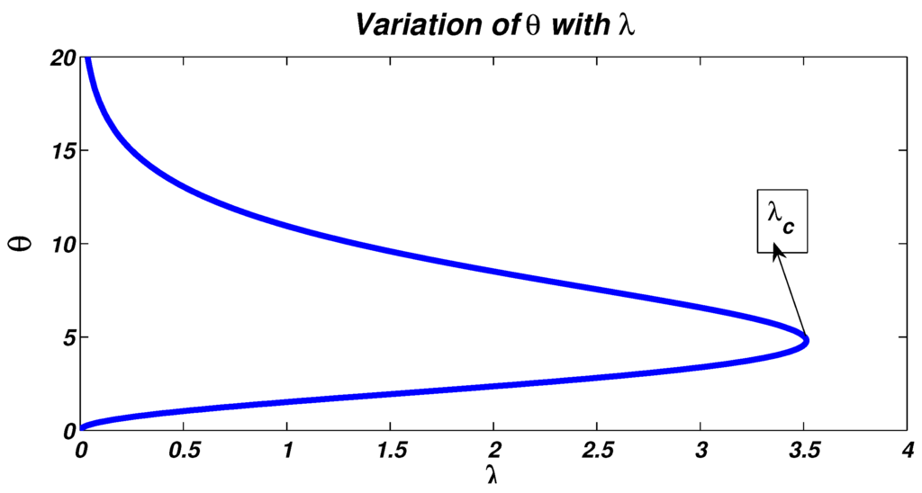
Figure 1. Variation of θ for different values of λ.

The finite dimensional problem using standard finite difference scheme is given by

$$F_j\left(U_j\right)=\frac{U_{j+1}-2U_j+U_{j-1}}{h^2}+\lambda exp{U}_j=0,j=1..N-1$$

(31)

with discrete boundary conditions $U_0=U_N=0$ and the step size $h=1/N$. There are $N-1$ unknowns ($n=N-1$). The Jacobian is a sparse matrix and its typical number of nonzero per row is three. It is known that the finite difference scheme converges to the lower solution of the 1-D Bratu using the starting vector $U^{\left(0\right)}={(0,0,..,0)}^T$.

We use $N=101$ ($n=100$) and test for 350 λ’s in the interval $(0,3.5]$ (interval width = 0.01). For each λ, we let $M_{\lambda }$ be the minimum number of iterations for which $\parallel U_j^{(k+1)}-U_j^{\left(k\right)}{\parallel }_2<1e-13$, where the approximation $U_j^{\left(k\right)}$ is calculated correct to 14 decimal places. Let $\overline{M_{\lambda }}$ be the mean of iteration number for the 350 λ’s.

Table 3. Comparison of number of λ’s in different methods for 1-D Bratu problem.

Method	$M=2$	$M=3$	$M=4$	$M=5$	$M>5$	$\overline{M_{\lambda }}$
$2^{nd}NM$	0	12	114	143	81	4.92
$3^{rd}HM$	0	140	206	2	2	3.62
$4^{th}SGS$	4	237	100	8	1	3.33
$4^{th}HM$	4	234	103	7	2	3.35
$6^{th}CHMT$	3	213	124	8	2	3.42
$6^{th}HM$	35	281	32	1	1	3.00

Table 3. Comparison of number of λ’s in different methods for 1-D Bratu problem.

Method	$M=2$	$M=3$	$M=4$	$M=5$	$M>5$	$\overline{M_{\lambda }}$
$2^{nd}NM$	0	12	114	143	81	4.92
$3^{rd}HM$	0	140	206	2	2	3.62
$4^{th}SGS$	4	237	100	8	1	3.33
$4^{th}HM$	4	234	103	7	2	3.35
$6^{th}CHMT$	3	213	124	8	2	3.42
$6^{th}HM$	35	281	32	1	1	3.00

Figure 2 and Table 3 give the results for the 1-D Bratu problem, where M represents number of iterations for convergence. It can be observed from the six methods considered in Table 3 that as λ increases to its critical value, the number of iterations required for convergence increase. However, as the order of method increases, the mean of iteration number decreases. The $6^{th}HM$ is the most efficient method among the six methods because it has the lowest mean iteration number and the highest number of λ converging in 2 iterations.

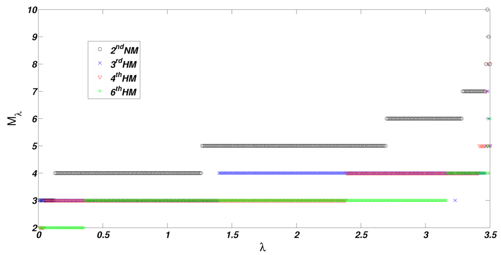
Figure 2. Variation of number of iteration with λ for the $2^{nd}NM$, $3^{rd}HM$, $4^{th}HM$ and $6^{th}HM$ methods.

For each λ, we find the minimum order of the ${(2r+4)}^{th}$HM family so that we reach convergence in 2 iterations and the results are shown in Figure 3. It can be observed that as the value of λ increases, the value of p required for convergence in 2 iterations also increases. For $\lambda \in [0.01,0.04]$, we require $p=4$ ($4^{th}HM$). For $\lambda \in [0.05,0.35]$, we require $p=6$ ($6^{th}HM$). For $\lambda \in [0.36,0.83]$, we require $p=8$ ($8^{th}HM$). For $\lambda \in [0.84,1.29]$, we require $p=10$ (${10}^{th}HM$). For $\lambda \in [1.30,1.66]$, we require $p=12$ (${12}^{th}HM$). For $\lambda \in [1.66,1.95]$, we require $p=14$ (${14}^{th}HM$). For $\lambda \in [1.96,2.19]$, we require $p=16$ (${16}^{th}HM$). For $\lambda \in [2.20,2.37]$, we require $p=18$ (${18}^{th}HM$). For $\lambda \in [2.38,2.52]$, we require $p=20$ (${20}^{th}HM$). For $\lambda \in [2.53,2.64]$, we require $p=22$ (${22}^{th}HM$) and so on. We notice that the width of the interval decrease and the order of the family is very high as λ tends to its critical value. Finally, for $\lambda =3.5$, we require $p=260$ to reach convergence in 2 iterations.

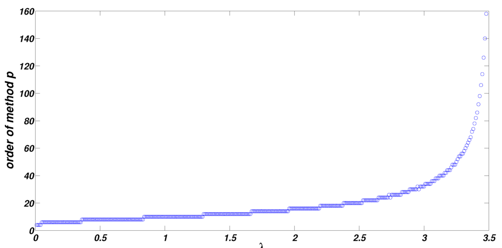
Figure 3. Order of the ${(2r+4)}^{th}$HM family for each λ.

5. Conclusion

In this work, we have proposed a fourth order method and its multi-step version having higher order convergence using weight functions to solve systems of nonlinear equations. The proposed schemes do not require the evaluation of second or higher order Fréchet derivatives to reach fourth order or higher order of convergence. We have tested a few examples using the proposed schemes and compared them with some known schemes, which illustrate the superiority of the new schemes. Finally, the proposed new methods have been applied on a practical problem called the 1-D Bratu problem. The results obtained are interesting and encouraging for the new methods. Hence, the proposed methods can be considered competent enough to some of the existing methods.

References

- Ostrowski, A.M. Solutions of Equations and System of Equations; Academic Press: New York, NY, USA, 1960. [Google Scholar]
- Homeier, H.H.H. On Newton-type methods with cubic convergence. Comp. Appl. Math. 2005, 176, 425–432. [Google Scholar] [CrossRef]
- Babajee, D.K.R. Analysis of Higher Order Variants of Newton’s Method and Their Applications to Differential and Integral Equations and in Ocean Acidification. Ph.D. Thesis, University of Mauritius, Moka, Mauritius, October 2010. [Google Scholar]
- Noor, M.A.; Waseem, M. Some iterative methods for solving a system of nonlinear equations. Comput. Math. Appl. 2009, 57, 101–106. [Google Scholar] [CrossRef]
- Sharma, J.R.; Guha, R.K.; Sharma, R. An efficient fourth order weighted-Newton method for systems of nonlinear equations. Numer. Algor. 2013, 62, 307–323. [Google Scholar] [CrossRef]
- Cordero, A.; Hueso, J.L.; Martinez, E.; Torregrosa, J.R. Increasing the convergence order of an iterative method for nonlinear systems. Appl. Math. Lett. 2012, 25, 2369–2374. [Google Scholar] [CrossRef]
- Babajee, D.K.R. On a two-parameter Chebyshev-Halley-like family of optimal two-point fourth order methods free from second derivatives. Afr. Mat. 2015, 26, 689–697. [Google Scholar] [CrossRef]
- Buckmire, R. Investigations of nonstandard Mickens-type finite-difference schemes for singular boundary value problems in cylindrical or spherical coordinates. Num. Meth. P. Diff. Eqns. 2003, 19, 380–398. [Google Scholar] [CrossRef]
- Babajee, D.K.R.; Kalyanasundaram, M.; Jayakumar, J. A family of higher order multi-point iterative methods based on power mean for solving nonlinear equations. Afr. Mat. 2015. [Google Scholar] [CrossRef]
- Cordero, A.; Hueso, J.L.; Martinez, E.; Torregrosa, J.R. A modified Newton-Jarratt’s composition. Numer. Algor. 2010, 55, 87–99. [Google Scholar] [CrossRef]
- Ortega, J.M.; Rheinbolt, W.C. Iterative Solution of Nonlinear Equations in Several Variables; Academic Press: New York, NY, USA, 1970. [Google Scholar]
- Cordero, A.; Torregrosa, J.R. Variants of Newton’s method using fifth-order quadrature formulas. Appl. Math. Comp. 2007, 190, 686–698. [Google Scholar] [CrossRef]
- Frontini, M.; Sormani, E. Third-order methods from Quadrature Formulae for solving systems of nonlinear equations. Appl. Math. Comp. 2004, 140, 771–782. [Google Scholar] [CrossRef]
- Odejide, S.A.; Aregbesola, Y.A.S. A note on two dimensional Bratu problem. Kragujevac J. Math. 2006, 29, 49–56. [Google Scholar]
© 2015 by the authors; licensee MDPI, Basel, Switzerland. This article is an open access article distributed under the terms and conditions of the Creative Commons Attribution license (http://creativecommons.org/licenses/by/4.0/).