Article

MAKHA—A New Hybrid Swarm Intelligence Global Optimization Algorithm

1
Department of Chemical Engineering, Faculty of Engineering, Cairo University, Giza 12613, Egypt
2
Department of Petroleum and Energy Engineering, American University in Cairo, New Cairo 11835, Egypt
3
Department of Chemical Engineering, Aguascalientes Institute of Technology, Aguascalientes 20256, Mexico
*
Author to whom correspondence should be addressed.
These authors contributed equally to this work.
Algorithms 2015, 8(2), 336-365; https://doi.org/10.3390/a8020336
Submission received: 2 April 2015 / Revised: 1 June 2015 / Accepted: 3 June 2015 / Published: 19 June 2015

Abstract

:
The search for efficient and reliable bio-inspired optimization methods continues to be an active topic of research due to the wide application of the developed methods. In this study, we developed a reliable and efficient optimization method via the hybridization of two bio-inspired swarm intelligence optimization algorithms, namely, the Monkey Algorithm (MA) and the Krill Herd Algorithm (KHA). The hybridization made use of the efficient steps in each of the two original algorithms and provided a better balance between the exploration/diversification steps and the exploitation/intensification steps. The new hybrid algorithm, MAKHA, was rigorously tested with 27 benchmark problems and its results were compared with the results of the two original algorithms. MAKHA proved to be considerably more reliable and more efficient in tested problems.

1. Introduction

The use of stochastic global optimization methods has gained popularity in a wide variety of scientific and engineering applications as those methods have some advantages over deterministic optimization methods [1]. Those advantages include the lack of the need for a good initial guess and the ability to handle multi-modal and non-convex objective functions without the assumptions of continuity and differentiability.
Several stochastic methods have been proposed and investigated in challenging optimization problems using continuous variables. Such methods include simulated annealing, genetic algorithms, differential evolution, particle swarm optimization, harmony search, and ant colony optimization. In general, these methods may show different numerical performances and, consequently, the search for more effective and reliable stochastic global optimization methods is currently an active area of research. In particular, the Monkey Algorithm (MA) [2] and the Krill-Herd Algorithm (KHA) [3] are two new, nature-inspired stochastic optimization method that are gaining popularity in finding the global minimum of diverse science and engineering application problems. For example, MA and its variants were recently used for the power system optimization [4], the coordinated control of low frequency oscillation [5], and for finding optimal sensor placement in structural health monitoring [6,7,8]. KHA is a new method and has been used in network route optimization [9] and economic load dispatch [10].
Since the development of those two algorithms, some modifications have been proposed to improve their performance. The modifications often involved variations of the search rules or hybridization with other algorithms. For example, chaotic search methods were added to MA [11] and KHA [12,13,14] to improve their performance. MA modifications also included the use of new parameters that change their value during the optimization [11], changing the watch-jump process of MA to make use of information obtained by other monkeys [5], redesigning the MA steps to facilitate discrete optimization problems [15], and incorporating an asynchronous climb process [7]. Other KHA modifications included the addition of local Lévy-flight move [16], adapting KHA to discrete optimization [9], better exchange of information between top krill during motion calculation [17], and hybridization of KHA with Harmony Search [18] and Simulated Annealing [19].
Hybridization is an enhancement in optimization algorithms in which operators from a certain algorithm are combined with other operators from another algorithm to produce more reliable and effective synergistic entity and get better results than that of the main parent algorithms. For example, SA (simulated annealing) is trajectory-based technique that is better at intensification or exploitation; it can detect the best solution with high probability in a confined search space. On the other hand, GA (Genetic algorithm) is regarded as population-based algorithm, which carrys out a diversification process and identifies promising regions of the search space [20,21]. An integration of both algorithms generated the SA-GA hybrid, which outperformed simple GA and a Monte Carlo search in terms of reliability and efficiency of the results. The improved genetic algorithm was implemented to optimize the weight of a pressure vessel under the burst pressure constraint [22]. It was contrived to cope with the phenomena of stagnation in earlier and later stages so that the ability of GA to escape entrapment in local minimum was used and wisely associated with SA’s intensification behavior.
Other examples of hybrids display the enhancement in results better than their parent algorithms. Hybrid Evolutionary Firefly Algorithm (HEFA) is a combination of FA and DE (Differential evolution) in which population was initiated, fitness values were evaluated, population was sorted and then split to two halves, the fitter half follows the FA, while the worse half evolves with the DE. HEFA was able to outperform the parent algorithms and GA, but with a longer computation time than GA [23]. BF-PSO hybrid is composed of BFO (Bacterial Forage Optimization) and PSO (Particle Swarm optimization), which was formed to improve the BFO’s ability to tackle multi-modal functions [24]. ACO has been hybridized with a Pseudo-Parallel GA (PPGA) for solving set of optimization problems, and PPGA-ACO obtained successfully the best minimum with minimal computational effort as compared to PPGA, GA, and neural networks [25]. The HS-BA (Harmony Search and Bees Algorithm hybrid) made the best results on eight out of 14 data instances of the University Course Timetabling Problem (UCTP), as compared to VNS (Variable Neighborhood Search), BA (Bees Algorithm), and TS (Tabu Search) [26]. The explorative ability of FA was enhanced by adding GA, and the hybrid was tested on a number of benchmarks and gained better results than standard FA and a number of PSO variants. However, it was often either outperformed by, or at best comparable to, FAs that use Gaussian distribution (Brownian motion) instead of Lévy flights, or use learning automata for parameter adaptation [27]. For further reading about hybrid algorithms, their methods, and strategies, please refer to the following: GA and BFO [28,29], PSO and SA [30], GA and SA [31], ACO and TS [32], and GA and PSO [33].
In this study, a new hybrid stochastic optimization method was developed, which uses features from the two algorithms, MA and KHA. The aim of this paper is to present the new algorithm and to evaluate its performance in comparison with the original algorithms. The remainder of this paper is divided as follows: Section 2 and Section 3 introduce the Monkey Algorithm and the Krill Herd Algorithm, respectively. Section 4 introduces the proposed hybrid algorithm. The numerical experiments performed to evaluate the modification are presented in Section 5. The results of the numerical experiments are presented and discussed in Section 6. Finally, Section 7 summarizes the conclusions of this study.

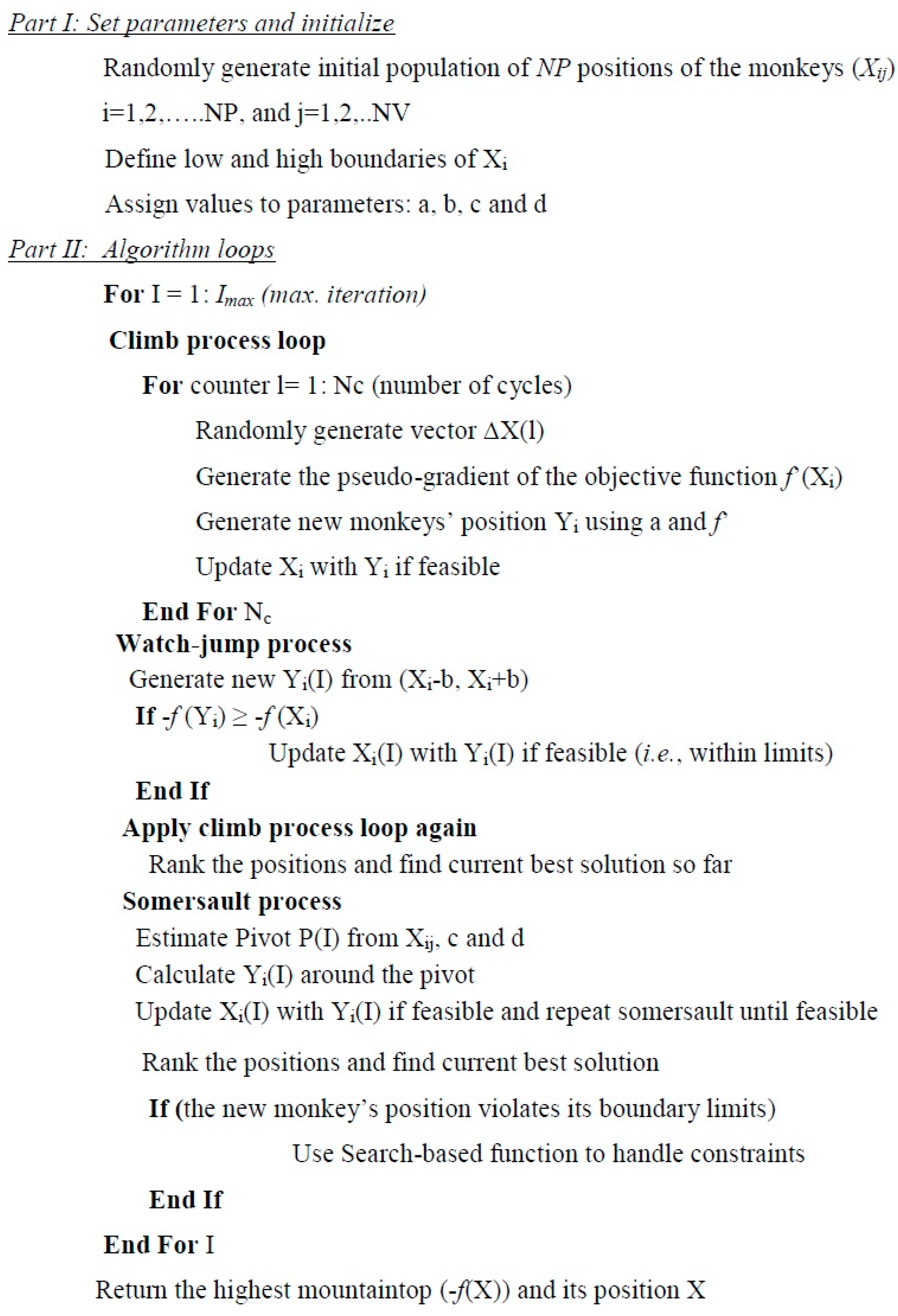
2. The Monkey Algorithm (MA)

This algorithm [2] mimics the process in which monkeys climb mountains to reach the highest point. The climbing method consists of three main processes:
1)
The climb process: In this exploitation process, monkeys search the local optimum solution extensively in a close range.
2)
The watch-jump process: In this process, monkeys look for new solutions with objective value higher than the current ones. It is considered an exploitation and intensification method.
3)
The somersault process: This process is for exploration and it prevents getting trapped in a local optimum. Monkeys search for new points in other search domains. In nature, each monkey attempts to reach the highest mountaintop, which corresponds to the maximum value of the objective function. The fitness of the objective function simulates the height of the mountaintop, while the decision variable vector is considered to contain the positions of the monkeys. Changing the sign of the objective function allows the algorithm to find the global minimum instead of the global maximum. The pseudo-code for this algorithm is shown in Figure 1.
Figure 1. The pseudo-code of the Monkey Algorithm (MA).
Algorithms 08 00336 g001
There are different equations for the somersault process. In this study, the somersault jump steps were as follows:
a)
Random generation of α from the somersault interval [c, d] where c and d governs the maximum distance that the monkey can somersault.
b)
Create a pivot P by the following equation:
P i = 1 N P 1 l = 1 N P ( i = 1 N P X l j X i j )
where P i = ( P 1 , P 2 , ... , P N V ) , NP is the population number and X is the monkey position.
c)
Get y (Monkey new position) from
Y i = X i + α | P i X i j |
d)
Update Xi with Yi if feasible (within boundary limits) or repeat until feasible.

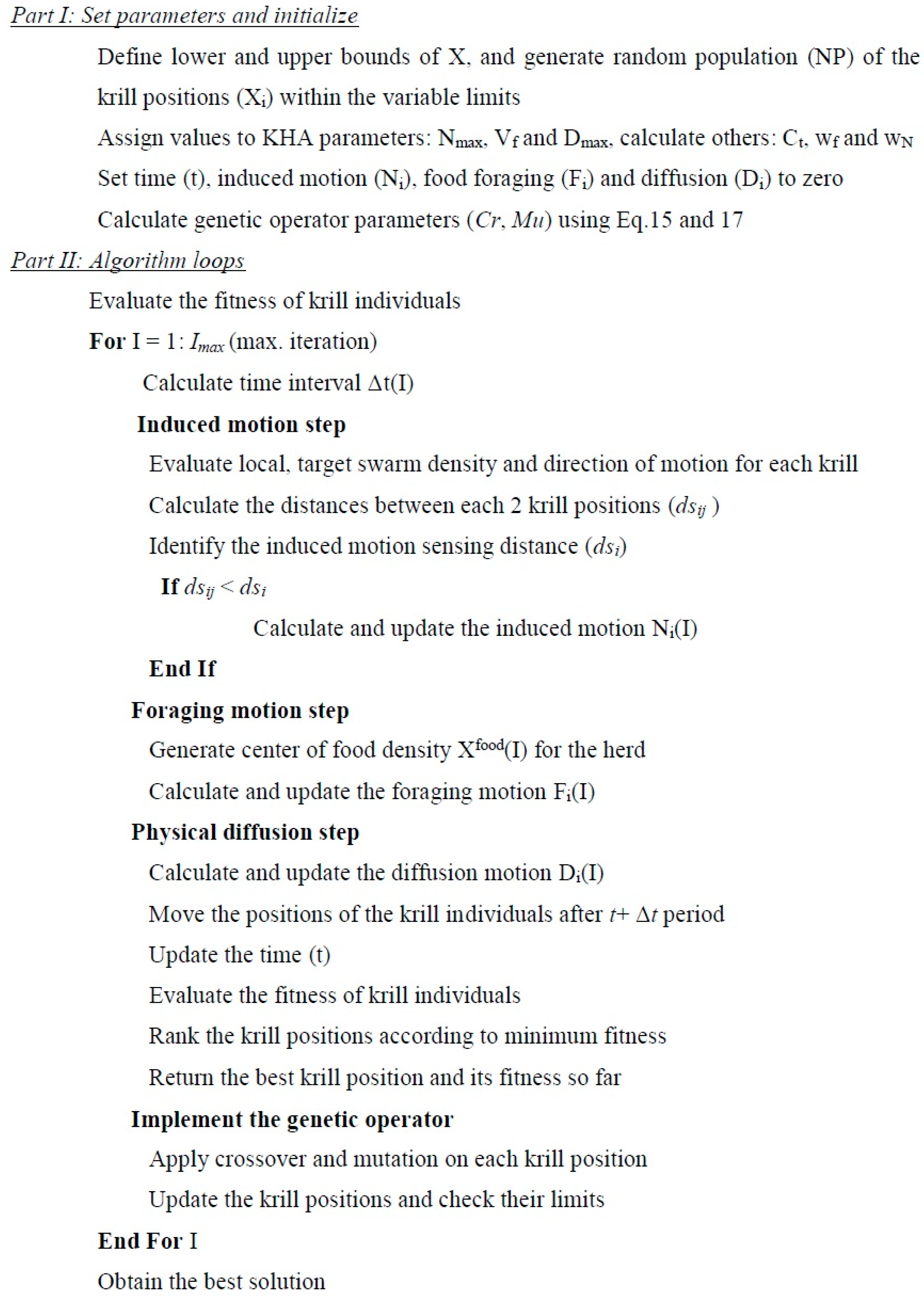
3. The Krill Herd Algorithm (KHA)

This bio-inspired algorithm [3] simulates the herding behavior of krill individuals. The values of the objective function correspond to the krill movements, which represent the minimum distances of each individual krill from food and from the highest density of the herd. The krill motion involves three main mechanisms,
a)
The movement induced by the presence of other individuals.
b)
The foraging activity.
c)
Random diffusion.
In addition, two adaptive genetic operators are used: Mutation and Crossover algorithms. In nature, when the predation action is made by predators, such as seals, penguins or sea birds, they remove krill individuals resulting in decreasing the krill density. Afterwards, the krill individuals increase their density and find food. So, the individual krill moves towards the best optimum solution as it searches for the highest density and food. The closer the distance to the highest density and food, the less value of the objective function is obtained. The objective function value of each individual krill is supposed to be an imaginary distance and contains a combination of the distance from food and from the highest density of the krill swarm. The individuals’ variables of the function are considered to be time-dependent positions of an individual krill, which are governed by the three mentioned features along with the genetic operator. The pseudo-code for this algorithm is shown in Figure 2.
It is important to note that there are four types of KHA: (1) KHA without any genetic operators (KHA I); (2) KH with crossover operator (KHA II); (3) KHA with mutation operator (KHA III); and (4) KH with crossover and mutation operators (KHA IV). In this study, KHA IV was used in solving the benchmark problems.
Figure 2. The pseudo-code of the Krill Herd Algorithm (KHA).
Algorithms 08 00336 g002

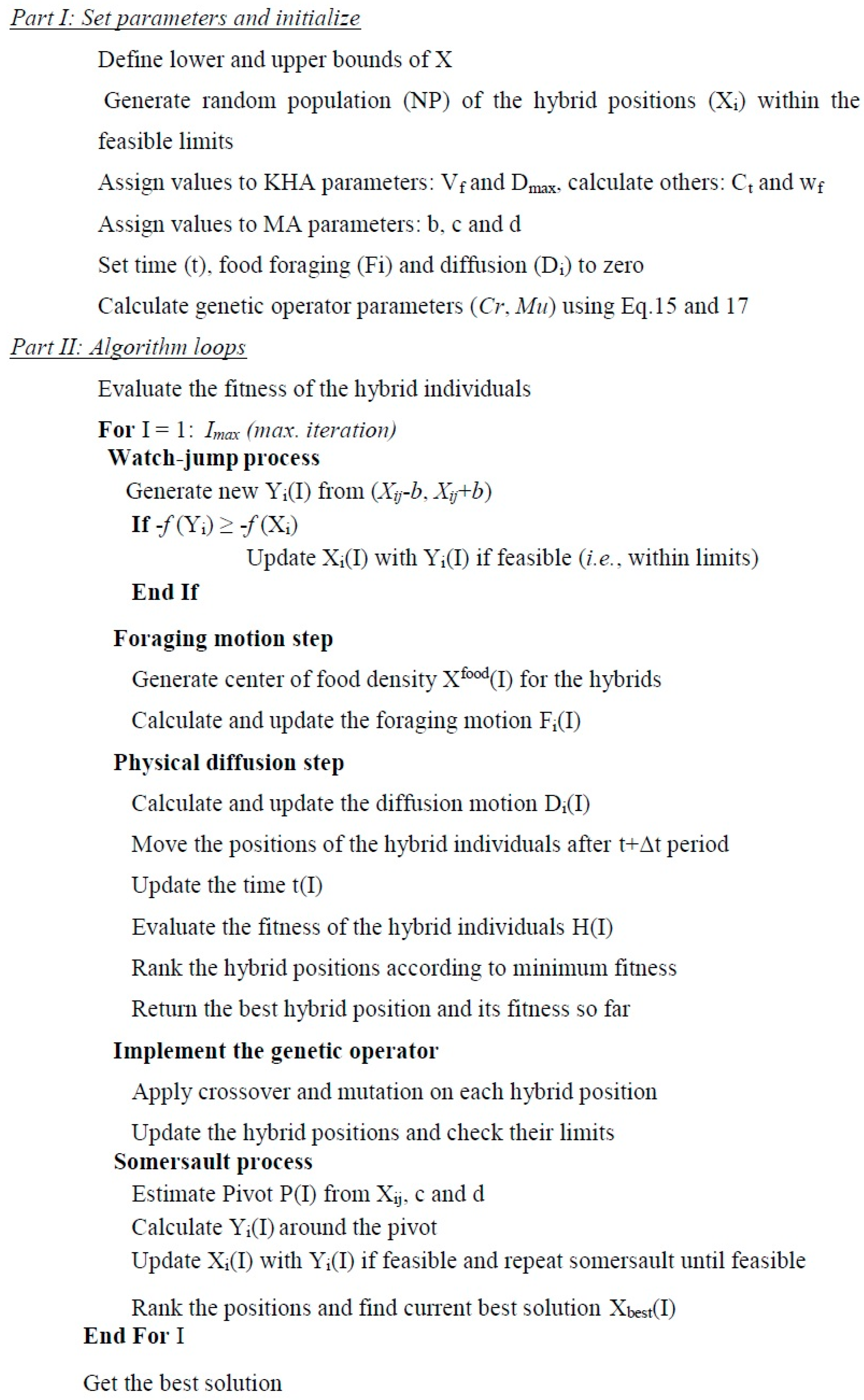
4. MAKHA Hybrid Algorithm

MAKHA is a new hybrid algorithm, which combines some of the mechanisms and processes of MA and KHA to get a reliable algorithm with appreciated performance. The steps of both algorithms include exploration/diversification and exploitation/intensification features as follows. The exploration/diversification features of MA are the somersault process and the watch-jump process, while for KHA, they are the physical random diffusion and the genetic operators. On the other hand, the exploitation/intensification features of MA are the climb and the watch-jump process, while for KHA, they are the induced motion and the foraging activity.
Both algorithms attempt to balance between exploration/diversification and exploitation/intensification features. MA has two exploration operators and two exploitation operators. The watch-jump process acts as both an exploration and an exploitation operator. The somersault operator is a high-performing diversification operator that makes a good use of the pivot function. Since MA is an exploration-dominant algorithm, the exploitation balance is brought to the algorithm by running the climb process twice per iteration. In each process, the MA algorithm uses a large number of cycles that reaches up to 2000 cycles in some problems. Increasing the number of cycles reduces the computational efficiency because it increases the number of function evaluations (NFE).
Even though KHA also has two exploration operators and two exploitation operators, its exploration component is not dominating because the physical random diffusion is a less efficient exploration operator than the somersault operator. Thus, the entrapment in local minima is more probable in KHA than in MA. The trapping problem can be addressed in the KHA by the use of two genetic operators (crossover and mutation), which appear in KHA IV algorithm. Since the foraging movement is a high-performing exploitation operator, KHA could be considered an exploitation-dominant algorithm.
An equal number of exploration and exploitation operators does not necessitate a balance between exploration and exploitation. The performance of operator is a critical factor. Assessing the performance of an operator can be done by replacing the exploration or exploitation operator in one algorithm with the same type of operator in the other algorithm. Testing the modified algorithms with benchmark problems can reveal whether or not the replaced operator was performing its function efficiently relative to the other operator.
To improve the performance of the algorithm such that the modified algorithm outperforms the two original algorithms, we aimed at using the best performing exploration and exploitation operators from the two algorithms. The hybrid algorithm, MAKHA, was constructed from the following processes:
  • The watch-jump process.
  • The foraging activity process.
  • The physical random diffusion process.
  • The genetic mutation and crossover process.
  • The somersault process.
The climb process, which consumes a high NFE, was not included in the hybrid algorithm. The random diffusion step was included in only one of MAKHA’s variant as explained below.
MAKHA was implemented in two different ways: MAKHA I, which does not use random diffusion; and MAKHA II, which uses the random diffusion step. It was found, as shown in the Results Section, that MAKHA I was more suitable for low-dimensional problems, while MAKHA II was better for the high-dimensional problems (NV = 50).
Figure 3. The pseudo-code of hybrid MAKHA.
Algorithms 08 00336 g003
The general pseudo-code for this algorithm is shown in Figure 3, while the equations used are as follows:
  • Initialization procedure:
    -
    Random generation of population in which the positions of the hybrid agent (monkey/krill) are created randomly, Xi = (Xi1, Xi2, …, Xi(NV)) where i = 1 to NP, which represents the number of hybrids, while NV represents the dimension of the decision variable vector.
  • The fitness evaluation and sorting:
    -
    Hi=f(Xi) where H stands for hybrid fitness and f is the objective function used.
  • The watch-jump process:
    -
    Random generation of Xi from (Xijb, Xij + b) where b is the eyesight of the hybrid (monkey in MA) which indicates the maximal distance the hybrid can watch and Yi = (Yi1, Yi2, …, Yi(NV)), which are the new hybrid positions.
    -
    If −f (Yi) ≥ −f (Xi) then update Xi with Yi if feasible (i.e., within limits).
  • Foraging motion:
    -
    Depends on food location and the previous experience about the location.
    -
    Calculate the food attractive β i f o o d and the effect of best fitness so far β i B e s t
    β i f o o d = C f o o d H ^ i , f o o d X ^ i , f o o d
    β i B e s t = H ^ i , i b e s t X ^ i , i b e s t
    where Cfood is the food coefficient, which decreases with time and is calculated from:
    C f o o d = 2 ( 1 I / I m a x )
    where I is the iteration number and Imax is the maximum number of iterations.
    -
    The center of food density is estimated from the following equation:
    X f o o d = i = 1 N P 1 H i X i i = 1 N P 1 H i
    and Hibest is the best previously visited position.
    -
    H ^ and X ^ are unit normalized values obtained from this general form:
    X ^ i , j = X j X i X j X i + ε
    H ^ i , j = H j H i H w o r s t H b e s t
    where ε is a small positive number that is added to avoid singularities. Hbest and Hworst are the best and the worst fitness values, respectively, of the hybrid agents so far. H stands for the hybrid fitness and was used as K symbol in krill herd method.
    -
    The foraging motion is defined as
    F i = V f β i + w f F i o l d
    where Vf is the foraging speed, wf is the inertia weight of the foraging motion in the range [0, 1], and F i o l d is the last foraging motion.
  • Physical diffusion:
    This is an exploration step that is used at high dimensional problem, then
    D i = D m a x ( 1 I / I m a x ) δ
    where Dmax is the maximum diffusion speed and δ is the random direction vector.
  • Calculate the time interval Δt
    Δ t = C t L = 1 N V ( U B L L B L )
    where Ct is constant.
  • The step for position is calculated through:
    d X i d t = F i + D i
    X i ( t + Δ t ) = X i ( t ) + Δ t d X i d t
    where d X i d t represents the velocity of the hybrid agent (Krill/Monkey).
  • Implementation of genetic operator:
    -
    Crossover
    X i , m = { X r , m ,   r a n d o m < C r X i , m ,   o t h e r w i s e }
    where r { 1 , 2 , ... , i 1 , i + 1 , ... , N P } and Cr is the crossover probability
    C r = 0.8 + 0.2 K ^ i , b e s t
    -
    Mutation
    X i , m = { X g b e s t , m + μ ( X p , m X q , m ) ,   r a n d o m < M u X i , m ,   o t h e r w i s e }
    where µ is a random number, p , q { 1 , 2 , ... , i 1 , i + 1 , ... , N P } and Mu is the mutation probability:
    M u = 0.8 + 0.05 H ^ i , b e s t
    H ^ i , b e s t = ( H i H g b ) / ( H w o r s t H g b )
    where Hgb is the best global fitness of the hybrid so far and Xgbest is its position.
  • The somersault process:
    -
    α is generated randomly from [c, d] where c and d are somersault interval. Two different implementations of the somersault process can be used:
    Somersault I
    -
    Create the pivot P [2]:
    P i = 1 N P i = 1 N P X i j  where  P i = ( P 1 , P 2 , ... , P N V )
    Y i = X i + α ( P i X i j )
    -
    Update Xi with Y if feasible or repeat until feasible.
    Somersault II
    -
    Create a pivot P by this equation used in MA:
    P i = 1 N P 1 l N P ( i = 1 N P X l j X i j )
    -
    Get Y (i.e., the hybrid new position)
    Y i = X i + α | P i X i j |
    -
    Update Xi with Y if feasible and repeat until feasible.
In summary, MAKHA offers more exploration than KHA and more exploitation than MA.

5. Numerical Experiments

Twenty-seven classical benchmark functions were used to evaluate the performance of MAKHA as compared to the original MA and KHA. Table 1 and Table 2 show the benchmark functions used along with their names, number of variables, variable limits and the value of the global minimum. Table 3 lists the parameters used in the three algorithms in which their values were set to give the best attainable results for each algorithm. A new parameter for MAKHA was defined as the midpoint between the lower boundary and the upper boundary of the decision variables X. It is calculated from this formula:
R = 0.5 L = 1 N V ( U B L L B L )
in which, according to the value R, certain values were assigned to MAKHA’s parameters, as seen in Table 3.
Table 1. Benchmark functions used for testing the performance of MA, KHA and MAKHA.
NameObjective Function
Ackley [34] f 1 = 20 ( 1 e 0.2 0.5 ( x 1 2 + x 2 2 ) ) e 0.5 ( cos 2 π x 1 + cos 2 π x 2 ) + e 1
Beale [35] f 2 = ( 1.5 x 1 + x 1 x 2 ) 2 + ( 2.25 x 1 + x 1 x 2 2 ) 2 + ( 2.625 x 1 + x 1 x 2 3 ) 2
Bird [36] f 3 = sin ( x 1 ) e ( 1 cos x 2 ) 2 + cos ( x 2 ) e ( 1 sin x 1 ) 2 + ( x 1 x 2 ) 2
Booth [35] f 4 = ( x 1 + 2 x 2 7 ) 2 + ( 2 x 1 + x 2 5 ) 2
Bukin 6 [35] f 5 = 100 | x 2 0.01 x 1 2 | + 0.01 | x 1 + 10 |
Carrom table [37] f 6 = [ cos x 1 cos x 2 e | 1 x 1 2 + x 2 2 / π | ] 2 / 30
Cross-leg table [37] f 7 = [ | sin ( x 1 ) sin ( x 2 ) e | 100 x 1 2 + x 2 2 / π | | + 1 ] 0.1
Generalized egg holder [35] f 8 = i = 1 m 1 { ( x i + 1 + 47 ) sin ( | x i + 1 + x i / 2 + 47 | ) + sin [ | x i ( x i + 1 + 47 ) | ] ( x i ) }
Goldstein–Price [38] f 9 = ( 1 + ( x 1 + x 2 + 1 ) 2 ( 19 14 x 1 + 3 x 1 2 14 x 2 + 6 x 1 x 2 + 3 x 2 2 ) ) ( 30 + ( 2 x 1 3 x 2 ) 2 ( 18 32 x 1 + 12 x 1 2 + 48 x 2 36 x 1 x 2 + 27 x 2 2 ) )
Himmelblau [39] f 10 = ( x 1 2 + x 2 11 ) 2 + ( x 2 2 + x 1 7 ) 2
Levy 13 [40] f 11 = sin 2 ( 3 π x 1 ) + ( x 1 1 ) 2 [ 1 + sin 2 ( 3 π x 2 ) ] + ( x 2 1 ) 2 [ 1 + sin 2 ( 2 π x 2 ) ]
Schaffer [37] f 12 = 0.5 + s i n 2 [ x 1 2 + x 2 2 ] 0.5 [ 0.001 ( x 1 2 + x 2 2 ) + 1 ] 2
Zettl [41] f 13 ) ( x 1 2 + x 2 2 2 x 1 ) 2 + x 1 4
Helical valley [42] f 14 = 100 [ ( x 3 10 θ ) 2 + ( x 1 2 + x 2 2 1 ) 2 ] + x 3 2 , 2 π θ = tan 1 ( x 1 x 2 )
Powell [43] f 15 = ( x 1 + 10 x 2 ) 2 + 5 ( x 3 x 4 ) 2 + ( x 2 2 x 3 ) 4 + 10 ( x 1 x 4 ) 4
Wood [44] f 16 = 100 ( x 1 2 x 2 ) 2 + ( x 1 1 ) 2 + ( x 3 1 ) 2 + 90 ( x 3 2 x 4 ) 2 + 10.1 [ ( x 2 1 ) 2 + ( x 4 1 ) 2 ] + 19.8 ( x 2 1 ) ( x 4 1 )
Extended Cube [45] f 17 = i = 1 m 1 100 ( x i + 1 x i 3 ) 2 + ( 1 x i ) 2
Shekel 5*[46] f 18 = i = 1 M ( j = 1 4 ( x j C j i ) 2 + β i ) 1
Sphere [47] f 19 = i = 1 m x i 2
Hartman 6 * [48] f 20 = i = 1 4 α i exp ( j = 1 6 A i j ( x j O i j ) 2 )
Griewank [49] f 21 = 1 4000 [ i = 1 m ( x i 100 ) 2 ] [ i = 1 m cos ( x i 100 i ) ] + 1
Rastrigin [50] f 22 = i = 1 m ( x i 2 10   cos ( 2 π x i ) + 10 )
Rosenbrock [51] f 23 = i = 1 m 1 100 ( x i + 1 x i 2 ) 2 + ( x i 1 ) 2
Sine envelope sine wave [37] f 24 = i = 1 m 1 { 0.5 + s i n 2 [ x i + 1 2 + x i 2 ] 0.5 [ 0.001 ( x i + 1 2 + x i 2 ) + 1 ] 2 }
Styblinski–Tang [52] f 25 = 0.5 i = 1 m ( x i 4 16 x i 2 + 5 x i )
Trigonometric [53] f 26 = i = 1 m [ m + i ( 1 cos x i ) sin x i j = 1 m cos x j ] 2
Zacharov [54] f 27 = i = 1 m x i 2 + ( i = 1 m 0 . 5 i x i ) 2 + ( i = 1 m 0 . 5 i x i ) 4
* Shekel and Hartman parameters were obtained from [36].
Table 2. Decision variables, global optimum of benchmark functions and number of iterations used for testing the performance of MA, KHA, and MAKHA.
Objective FunctionNVSearch DomainGlobal MinimumIterations
MAKHAMAKHA
Ackley2[−35, 35]02530001000
Beale2[−4.5, 4.5]02530001000
Bird2[−2π, 2π]−106.7652530001000
Booth2[−10, 10]02530001000
Bukin 62[−15, 3]02530001000
Carrom table2[−10, 10]−24.156812530001000
Cross-leg table2[−10, 10]−12530001000
Generalized egg holder2[−512, 512]−959.6412415,0005000
Goldstein-Price2[−2, 2]32530001000
Himmelblau2[−5, 5]02530001000
Levy 132[−10, 10]02530001000
Schaffer2[−100, 100]019915,0008000
Zettl2[−5, 5]−0.0037912530001000
Helical valley3[−1000, 1000]02530001000
Powell4[−1000, 1000]05060002000
Wood4[−1000, 1000]02530001000
Extended Cube5[−100, 100]02530001000
Shekel 54[0, 10]−10.15322530001000
Sphere5[−100, 100]07590001000
Hartman 66[0,1]−3.322372530001000
Griewank50[−600, 600]0124150005000
Rastrigin50[−5.12, 5.12]0124150005000
Rosenbrock50[−50, 50]0124150005000
Sine envelope sine wave50[−100, 100]0124150005000
Styblinski-Tang50[−5,5]−1958.2995124150005000
Trigonometric50[−1000, 1000]0124150005000
Zacharov50[−5,10]02530001000
Table 3. Selected values of the parameters used in the implementation of MA, KHA and MAKHA.
MethodConditionParameterSelected value
MA b1
R ≥ 100b10
c−1
d1
R ≥ 500c−10
R ≥ 500d30
NC30
KHA Dmax[0.002, 0.01]
Ct0.5
Vf0.02
Nmax0.01
wf and wN[0.1, 0.8]
MAKHA I b1
R < 2b0.5*R
R ≥ 100b10
c−0.1
d0.1
Dmax0
Ct0.5
Vf0.2
wf0.1
Somersault I is used
MAKHA II (NV = 50) b0.3*R
c−R
dR
Dmax[0.002, 0.01]
Ct0.5
Vf0.02
wf[0.1, 0.8]
Somersault II is used
The twenty-seven problems constitute a comprehensive testing of the reliability and effectiveness of the hybrid algorithm. Thirteen functions have two variables only, yet some of them are very difficult to optimize. Surface plots of eight of the two-variable functions are shown in Figure 4. Each problem was solved 30 times by each of the three algorithms. The best value at each iteration was recorded and the means of the best values were calculated amongst the 30 run as a function of the iteration number. The plots of the mean best values versus the number of function for the three algorithms provide a clear comparison of both the reliability and the efficiency of the algorithms. Reliability is represented by how far the algorithm predictions of the minimum are from the known global minimum, while efficiency is represented by the number of function evaluations needed for the calculation of this best value.
Figure 4. Surface plots of the two-variable benchmark functions used in this study: (a) Ackley, (b) Beale, (c) Booth, (d) Carrom table, (e) Cross-leg table, (f) Himmelblau, (g) Levy 13, and (h) Schaffer.
Algorithms 08 00336 g004aAlgorithms 08 00336 g004b
To complete the evaluation of the MAKHA in comparison with the original MA and KHA algorithms, we have employed the performance profile (PP) reported by Dolan et al. [55], who introduced PP as a tool for evaluating and comparing the performance of optimization software. In particular, PP has been proposed to represent compactly and comprehensively the data collected from a set of solvers for a specified performance metric. For instance, the number of function evaluations or computing time can be considered performance metrics for solver comparison. The PP plot allows visualization of the expected performance differences among several solvers and to compare the quality of their solutions by eliminating the bias of failures obtained in a small number of problems.
To introduce PP, consider ns solvers (i.e., optimization methods) to be tested over a set of np problems. For each problem p and solver s, the performance metric tps must be defined. In our study, reliability of the stochastic method in accurately finding the global minimum of the objective function is considered as the principal goal, and hence the performance metric is defined as
t p s = f c a l c f *
where f* is the known global optimum of the objective function and fcalc is the mean value of that objective function calculated by the stochastic method over several runs. In our study, fcalc is calculated from 30 runs to solve each test problem by each solver; note that each run is different because of the random number seed used and the stochastic nature of the method. So, the focus is on the average performance of stochastic methods, which is desirable for comparison purposes.
For the performance metric of interest, the performance ratio, rps, is used to compare the performance on problem, p, by solver, s, with the best performance by any solver on this problem. This performance ratio is given by
r p s = t p s min { t p s : 1 s n s }
The value of rps is 1 for the solver that performs the best on a specific problem p. To obtain an overall assessment of the performance of solvers on np problems, the following cumulative function for rps is used:
ρ s ( ς ) = 1 n p s i z e { p : r p s ζ }
where ρ(ς) is the fraction of the total number of problems, for which solver s has a performance ratio rps within a factor of ς of the best possible ratio. The PP of a solver is a plot of ρs(ς) versus ς; it is a non-decreasing, piece-wise constant function, continuous from the right at each of the breakpoints.
To identify the best solver, it is only necessary to compare the values of ρs(ς) for all solvers and to select the highest one, which is the probability that a specific solver will “win” over the rest of solvers used. In our case, the PP plot compares how accurately the stochastic methods can find the global optimum value relative to one another, and so the term “win” refers to the stochastic method that provides the most accurate value of the global minimum in the benchmark problems used.

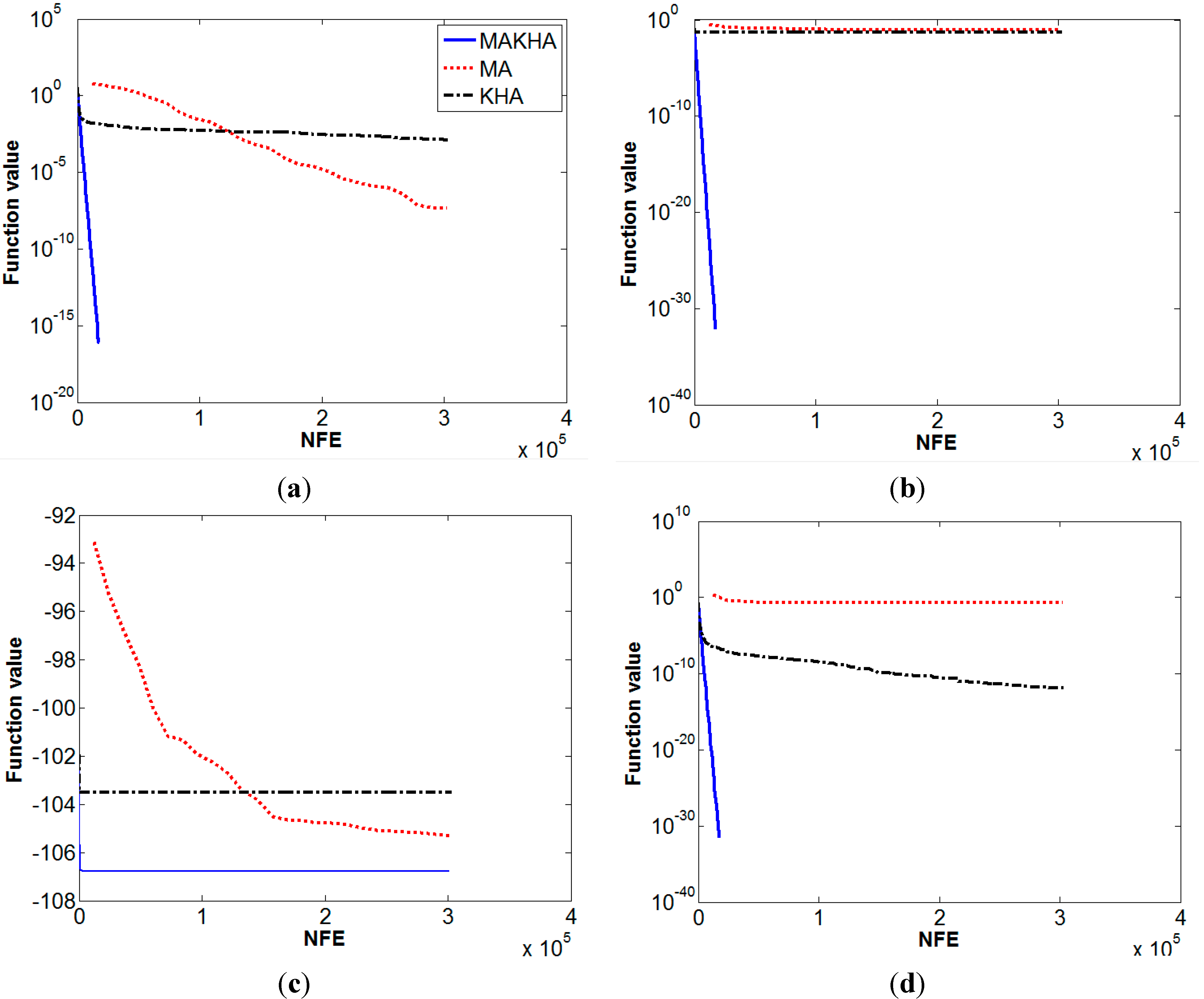
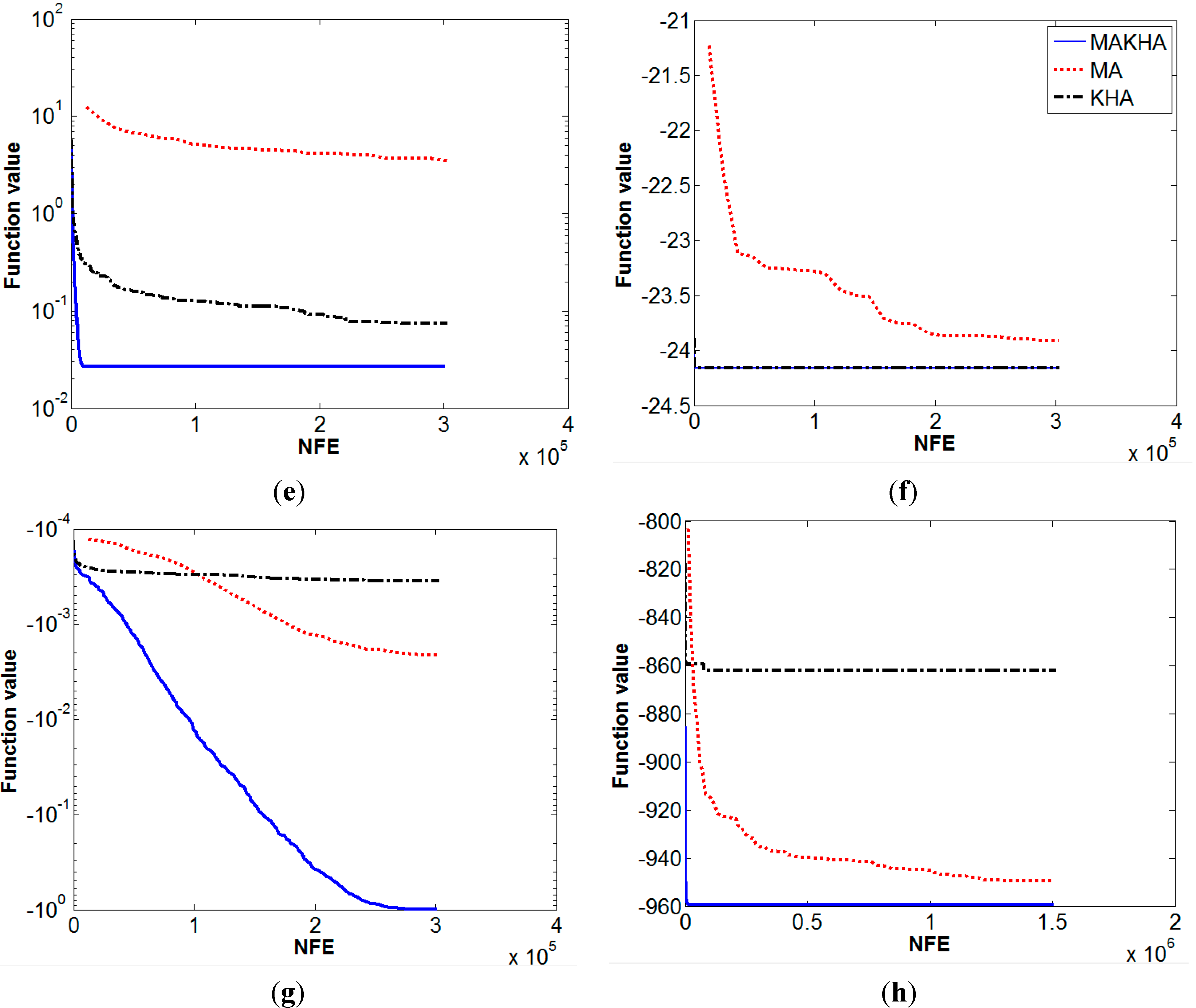
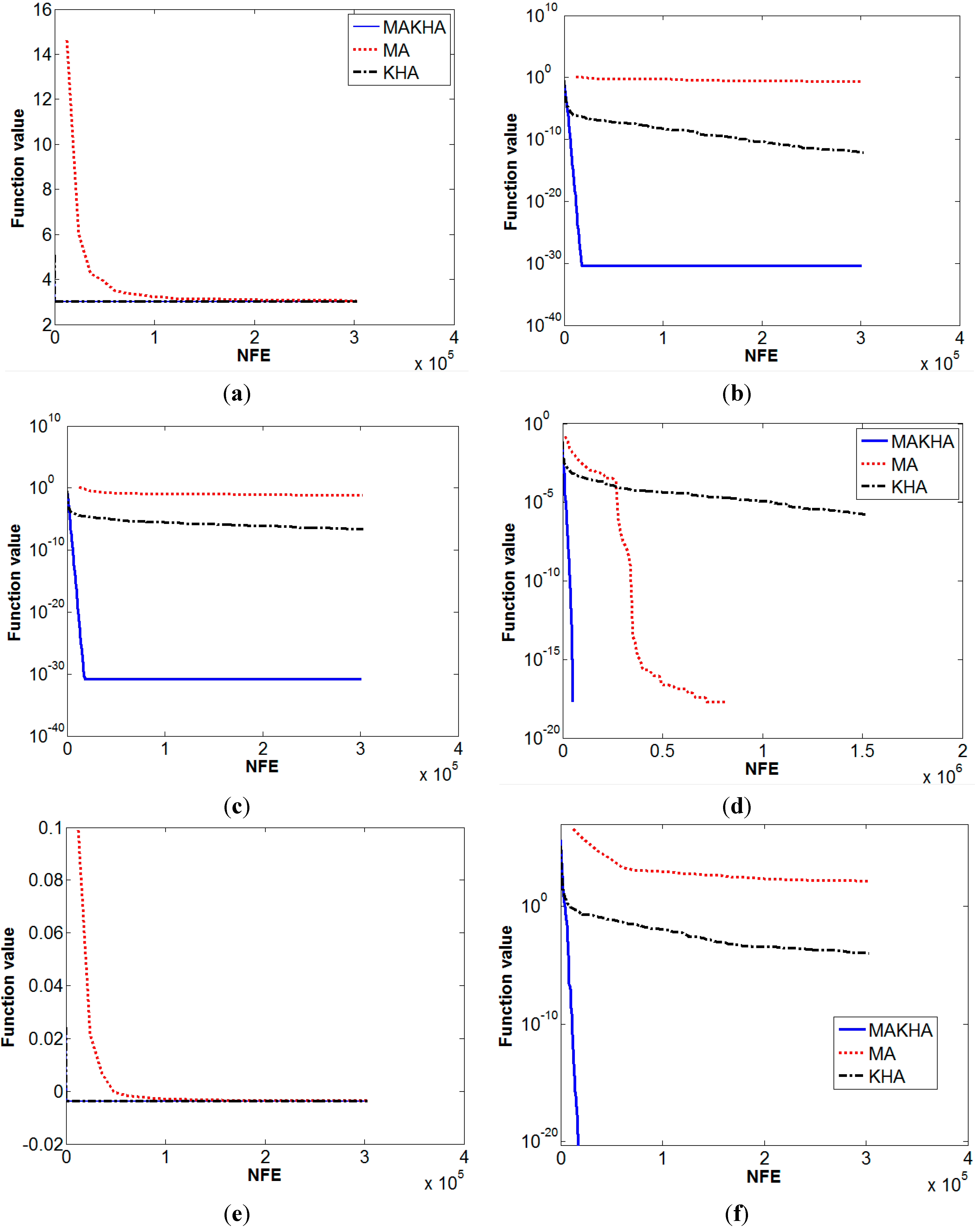
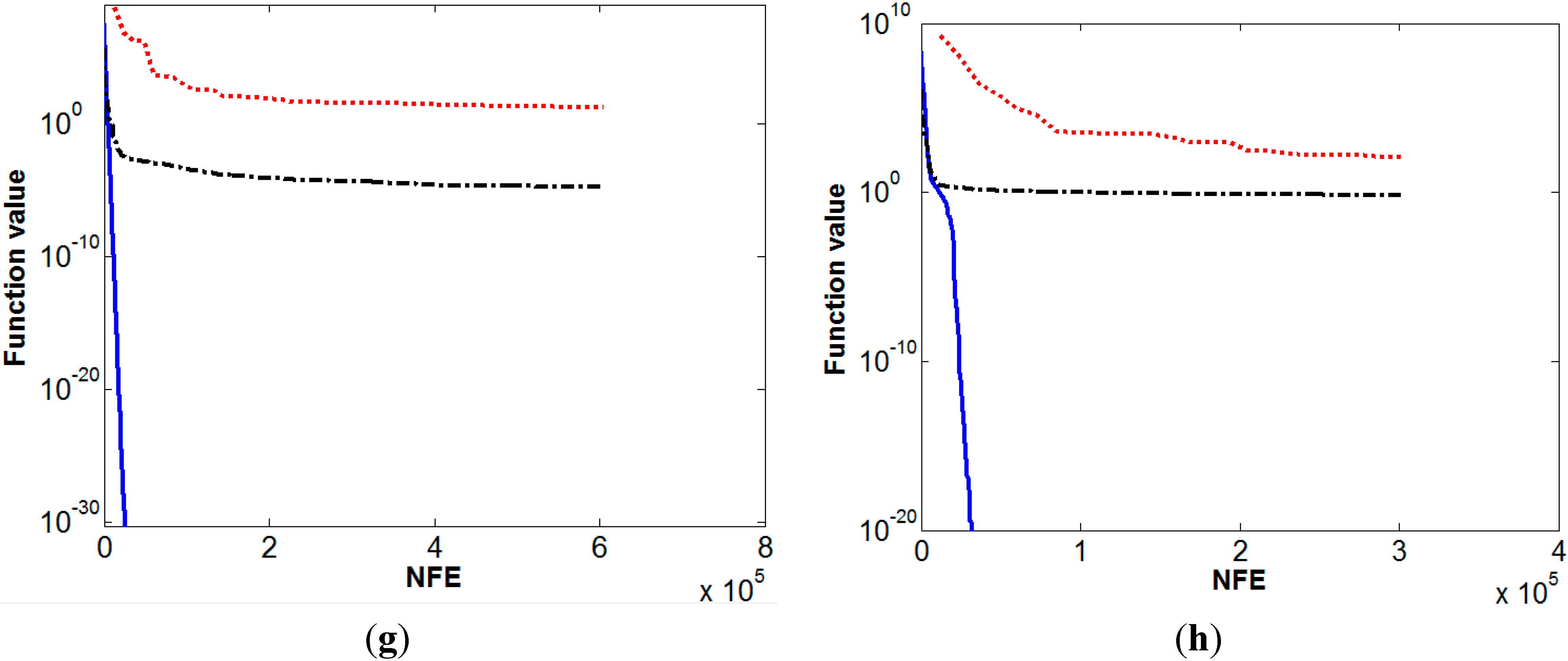
6. Results and Discussion

As stated, each of the numerical experiments was repeated 30 times with different random seeds for MAKHA and the original MA and KHA algorithms. Parameters used for stochastic algorithms are reported in Table 3. The objective function value at each iteration for each trial was recorded. The mean and the standard deviation of the function values were calculated at each iteration. The global optimum was considered to be obtained by the method if it finds a solution within a tolerance value of 10−10. The progress of the mean values is presented in Figure 5, Figure 6, Figure 7 and Figure 8 for each benchmark function and a brief discussion of those results follows.
The Ackley function has one minimum only. The global optimum was obtained using MAKHA and in relatively small number of function evaluations as shown in Figure 5a. MA and KHA were not able to obtain satisfactorily the global minimum. The best value obtained by MA was still improving by the end of the run, whereas KHA results were not.
This significant improvement in performance was also clear with the Beale function (Figure 5b). The Beale function has one minimum only, which was only obtained satisfactory by MAKHA. The performance pattern for the three methods was different for the Bird function, as depicted in Figure 5c. MAKHA arrived at the global minimum almost instantaneously. KHA was trapped in a local minimum, while MA was approaching the global minimum, but did not reach it after 300,000 function evaluations. For the Booth function, both MAKHA and KHA arrived at the global minimum but with an improvement in orders of magnitude for the efficiency of MAKHA. On the other hand, MA failed to arrive at the global minimum, as shown in Figure 5d. For Bukin 6 function, none of the three methods obtained the global minimum within the used tolerance. However, MAKHA performed better than KHA, which performed better than MA, as shown in Figure 5e.
MAKHA and KHA performed similarly for the Carrom table function, as they obtained the global minimum almost instantaneously, as shown in Figure 5f. MA could not achieve the global minimum even after 300,000 function evaluations. For the Cross-leg table function, MAKHA was the only method to obtain the global minimum, as shown in Figure 5g. Note that MA performed better than KHA after many NFE. MAKHA obtained the global minimum for the Generalized Eggholder function almost instantaneously, as depicted in Figure 5h. The other two methods were not able to obtain the global minimum but MA’s performance was significantly better than KHA’s.
Figure 5. Evolution of mean best values for MA, KHA and MAKHA for: (a) Ackley, (b) Beale, (c) Bird (d) Booth, (e) Bukin6 (f) Carrom table, (g) Cross-leg table, and (h) Generalized Eggholder functions.
Algorithms 08 00336 g005aAlgorithms 08 00336 g005b
For the Goldstein-Price function, all three algorithms obtained the global minimum, as depicted in Figure 6a. However, MAKHA and KHA were orders-of-magnitude more efficient than MA. For the Himmelblau function, MAKHA obtained the global minimum at low NFE, KHA obtained it at high NFE, and MA was not able to obtain it after 300,000 NFE, as shown in Figure 6b. This performance was almost exactly repeated with the Levy 13 function, as shown in Figure 6c. As for the Schaffer function, both MAKHA and MA converged to the global minimum within the used tolerance. MAKHA was more efficient than MA in terms of the NFE required to obtain the global minimum, as shown in Figure 6d. KHA failed to converge to the global minimum for this particular function. Figure 6e shows the evolution pattern for the Zettl function. MAKHA and KHA obtained the global minimum within a small NFE, while MA obtained it after considerably more NFE. The Helical Valley function has three variables. The evolution of the mean best values of the three algorithms is reported in Figure 6f and results showed that the performance of MAKHA was better than the other two algorithms. MAKHA efficiently obtained the global minimum, while the other two could not, with KHA performing better than MA. This convergence performance is almost exactly repeated with the two four-variable functions, the Powell function (Figure 6g) and with the Wood function (Figure 6h).
Figure 6. Evolution of mean best values for MA, KHA and MAKHA for: (a) Goldstein–Price (b) Himmelblau, (c) Levy 13, (d) Schaffer functions, (e) Zettl, (f) Helical Valley, (g) Powell and (h) Wood.
Algorithms 08 00336 g006aAlgorithms 08 00336 g006b
The evolution of the mean best values of the three algorithms for the five-variable functions, which are the Extended Cube, Shekel and Sphere functions, are reported in Figure 7a–c, respectively. For the Extended Cube function, MAKHA was able to obtain the global minimum, while the other two methods failed to converge to the global minimum. For the Shekel function, MAKHA obtained the global minimum very efficiently, as compared to MA, which obtained it at a higher NFE. KHA failed to converge to the global minimum for this function. A relative close pattern is repeated with the five-variable sphere function. Hartman function is a fifty-variable function and its results are depicted in Figure 7d. MAKHA and KHA converged to the global minimum efficiently, while MA failed to achieve it after 300,000 function evaluations. For the Griewank function, shown in Figure 7e, the three algorithms failed to converge to the global minimum. However, MAKHA performance was considerable better than the performance of the other two algorithms, which performed similarly. The Rastrigin function is one of the three functions in which MAKHA was not the top performer. The results for the Rastrigin function are reported in Figure 7f. The three methods did not obtain the global minimum. However, MA performed better than MAKHA, which in turn performed better than KHA. For the Rosenbrock function, whose results are shown in Figure 7g, the three algorithms did not obtain the global minimum, within the acceptable tolerance, with 1,500,000 function evaluations. However, the best value obtained by MAKHA is seven orders-of-magnitude better than that obtained by the other two algorithms. Sine Envelope Sine function is the second function in which MAKHA did not outperform MA, see Figure 7h. MA was the only method to achieve the global minimum. MAKHA’s performance was significantly better than KHA’s performance.
Figure 7. Evolution of mean best values for MA, KHA and MAKHA for: (a) Extended cube, (b) Shekel, (c) Sphere, (d) Hartman, (e) Griewank (f) Rastrigin, (g) Rosenbrock, and (h) Sine Envelope Sine functions.
Algorithms 08 00336 g007
Figure 8a–c shows the results of the mean best value obtained by the three algorithms for Styblinski–Tang, Trigonometric, and Zacharov functions, respectively. MAKHA was the only method to obtain the global minimum for Styblinski-Tang function and it did efficiently as measured by NFE. MA outperformed KHA for this particular function. The same pattern was obtained with the Trigonometric function as depicted in Figure 8b. The Zacharov function is the third function, which MAKHA did not outperform MA, as shown in Figure 8c.
Figure 8. Evolution of mean best values for MA, KHA and MAKHA for: (a) Styblinski-Tang, (b) Trigonometric and (c) Zacharov functions.
Algorithms 08 00336 g008
Table 4 shows a summary of the performance results for the twenty-seven benchmark problems. MAKHA has outperformed its parent algorithms in the majority of the benchmark problems studied. Best global values are shown in bold. The performance profiles reported in Figure 9 summarize the results of the MAKHA evaluation in comparison with the two original algorithms. MAKHA was the best algorithm in 24 out of the 27 cases considered. In several cases, the hybrid algorithm was the only algorithm that obtained the global minimum. Also, due to its efficient exploration and exploitation components, it converges to the global minimum with less NFE than the original two algorithms.
Table 4. Values of the mean minima (fcalc) and standard deviations (σ) obtained by the MAKHA, MA and KHA algorithms for the benchmark problems used in this study.*
Numerical Performance of
MAKHAMAKHA
Objective functionfcalcσfcalcσfcalcσ
Ackley4.8E−800.00129000
Beale0.0840.1250.05080.19300
Bird−105.3261.45−103.527.4−106.76450
Booth0.1790.1721.28E−12000
Bukin 63.4871.770.0740.0290.02670.0157
Carrom table−23.91380.436−24.15680−24.15680
Cross-leg table−0.0024E−3−0.000350−0.99850
Generalized egg holder−949.580−862.10−959.6410
Goldstein-Price3.0510.0553030
Himmelblau0.1790.1877.4E−1303.7E−310
Levy 130.06160.082.1E−701.35E−310
Schaffer001.7E−6000
Zettl−0.00371E−3−0.003790−0.003790
Helical valley1362509.8E−53E−300
Powell18.46491.9E−5000
Wood113.62560.6981.600
Extended Cube3.5680.81.6585.2800
Shekel 5−10.1390.06−5.3843.1−10.15320
Sphere1.4E−1401E−10000
Hartman 6−2.74990.2−3.25870.06−3.26270.06
Griewank0.01650.0320.07690.0958.4E−80
Rastrigin1.3E-9089.3848.386.47E−60
Rosenbrock47.457.552.59318.971E−50
Sine envelope sine wave3.3E−11016.1075.943.46E−60
Styblinski-Tang−1916.8428.1−1645.4236.9−1958.310
Trigonometric1.35E−50285.43545.500
Zacharov1.46E−1001E−35.5E−38.4E−60
* Bold numbers represent the best global minimum value obtained for each function.
Figure 9. Performance profiles of the MAKHA, MA, and KHA methods for the global optimization of the twenty-seven benchmark problems used in this study.
Algorithms 08 00336 g009
The results of new proposed hybrid were promising that could be attributed to the combination of some of the mechanisms and processes of MA and KHA together to produce a reliable algorithm with appreciated performance. The procedures of both algorithms include exploration/diversification and exploitation/intensification features as follows:
(a)
Exploration or diversification feature: The watch-jump process (MA), physical random diffusion (KHA), the somersault process (MA), and genetic operators (KHA).
(b)
Exploitation or intensification feature: The climb process (MA), the watch-jump process (MA), the induced motion (KHA), and the foraging activity (KHA).
Both algorithms (MA and KHA) make a good compromise and balance between exploration/diversification and exploitation/intensification features. However, MAKHA uses the best setup of efficient operators, which are capable of producing the previous promising results.

7. Conclusions

In this paper, we propose a new hybrid algorithm, which is based on two bio-inspired swarm intelligence global stochastic optimization methods, the Monkey Algorithm and the Krill Herd Algorithm. The hybridization made use of the efficient components in each of the two original algorithms. It aimed to provide a better balance between exploration/diversification steps and exploitation/intensification steps to more efficiently and more reliably solve a wide range of problems in comparison with the its parent algorithms. This hybrid method was evaluated by attempting to find the global optimum of twenty-seven benchmark functions. The newly developed MAKHA algorithm led to improved reliability and effectiveness of the algorithm in the vast majority of the benchmark problems. In many cases, the global minimum could not be obtained via the original algorithms, but was easily obtained by the new method.
The authors are currently working on the improvement of MAKHA by decreasing the number of its parameters, and increasing its reliability and efficiency in solving difficult thermodynamic problems. The performance of MAKHA is compared to the performance of other algorithms thath have high reliability in solving these kinds of problems.

Supplementary Materials

Supplementary materials can be accessed at: https://www.mdpi.com/1999-4893/8/2/336/s1.

Acknowledgments

Authors acknowledge the support provided by the Cairo University (Egypt) and Instituto Tecnologico de Aguascalientes (Mexico).

Author Contributions

This research study was performed as a part of the Masters thesis of Ahmed M. E. Khalil at Cairo University. He suggested the hybrid algorithm to his supervisor, Seif-Eddeen K. Fateen, who contributed with ideas on implementation and evaluation of the algorithm. Adrian Bonilla-Petriciolet, a collaborator with Fateen on the use of stochastic global optimization, analyzed the data. Khalil and Fateen wrote the paper, while Bonilla-Petriciolet reviewed the manuscript and provided valuable comments to improve the paper.

Conflicts of Interest

The authors declare no conflict of interest.

Abbreviations

A
Hartman’s recommended constants
a
Pseudo-gradient monkey step
b
Eyesight of the monkey (hybrid), which indicates the maximum distance the monkey (hybrid) can watch.
C
Shekel’s recommended constants
Cfood
Food coefficient
Cr
Crossover probability
Ct
Empirical and experimental Constants (Time constant)
c
Somersault interval
Di
Physical diffusion of krill (hybrid) number i
Dmax
Maximum diffusion speed
d
Somersault interval
dsi
Sensing distance of the krill
dsij
Distance between each 2 krill positions
f
Objective function
Fi
Foraging motion
G
Global minimum
H
Fitness value of the hybrid in MAKHA
I, i, j and l
Counters for any value
K
Fitness value of the krill in KHA
M
Number of local minima in Shekel function
LB
Lower boundaries and low limit of decision variable
Mu
Mutation probability
m
Dimension of the problem, i.e., number of variables.
N
Induced speed for KHA
Nc
Number of climb cycles
Nmax
Maximum induced speed
NP
Population size (number of points)
NV
Dimension of the problem, i.e., number of variables.
n
A counter
np
Number of problems
ns
Number of solvers
O
Hartman’s recommended constants
P
Pivot value
R
The half range of boundaries between the lower boundary and the upper boundary of the decision variables (X)
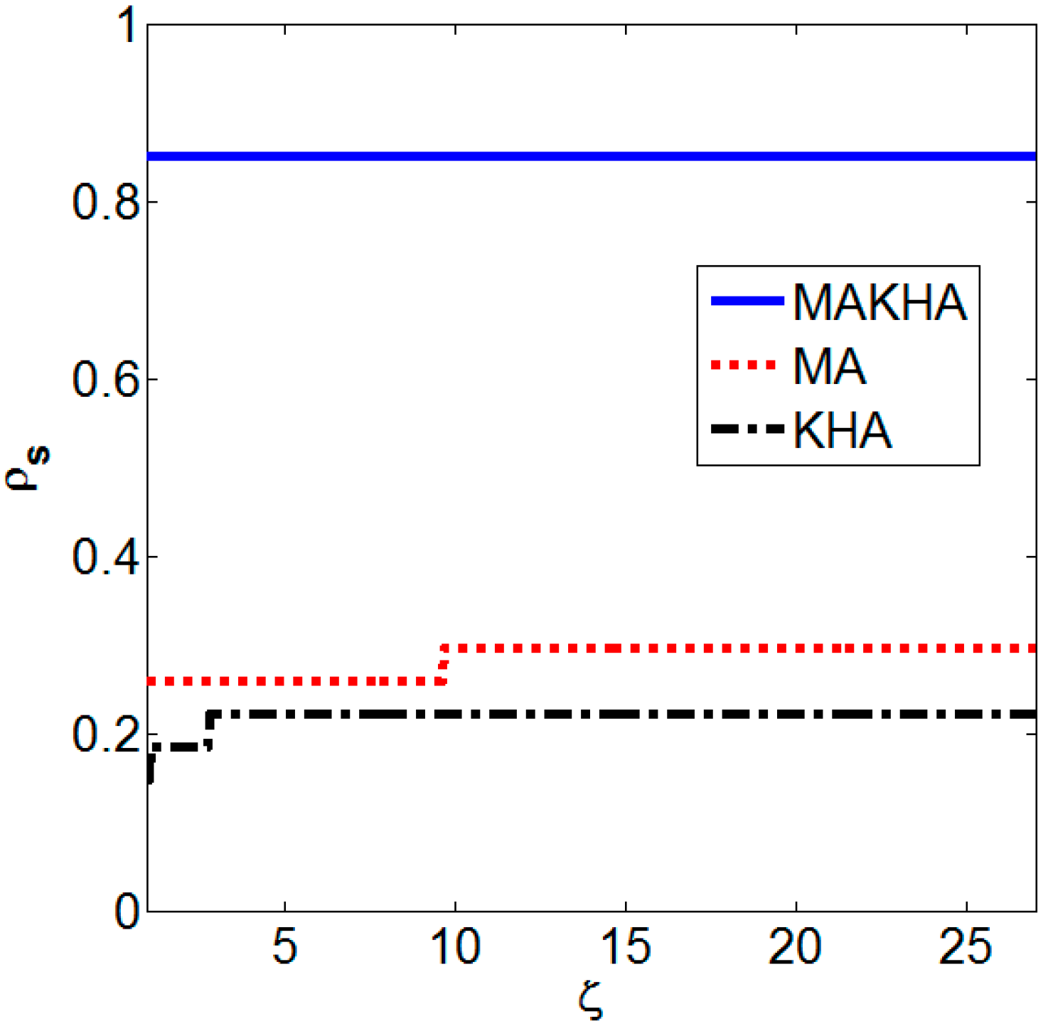
rps
The performance ratio
T
Time taken by krill or hybrid
tps
Performance metric
UB
Upper boundaries and high limit of decision variable
Vf
Foraging speed
wf or wN
Inertia weight
X
Decision variable matrix
Xfood
Centre of food density
x
Decision variable
Y
Decision variable matrix

Greek Letters

α
Somersault interval random output.
β
Shekel’s recommended constant
βfood
Food attractive factor
δ
Random direction vector
∆t
Incremental period of time
ε
Small positive number to avoid singularity
ζζ
The simulating value of rps
ζmax
The maximum assumed value of rps
ρ
The cumulative probabilistic function of rps and the fraction of the total number of problems
σ
Standard deviation
ςς
The counter of ρ points

References

  1. Floudas, C.A.; Gounaris, C.E. A review of recent advances in global optimization. J. Glob. Optim. 2009, 45, 3–38. [Google Scholar] [CrossRef]
  2. Zhao, R.; Tang, W. Monkey algorithm for global numerical optimization. J. Uncertain Syst. 2008, 2, 165–176. [Google Scholar]
  3. Gandomi, A.H.; Alavi, A.H. Krill herd: A new bio-inspired optimization algorithm. Commun. Nonlinear Sci. Numer. Simul. 2012, 17, 4831–4845. [Google Scholar] [CrossRef]
  4. Ituarte-Villarreal, C.M.; Lopez, N.; Espiritu, J.F. Using the Monkey Algorithm for Hybrid Power Systems Optimization. Procedia Comput. Sci. 2012, 12, 344–349. [Google Scholar] [CrossRef]
  5. Aghababaei, M.; Farsangi, M.M. Coordinated Control of Low Frequency Oscillations Using Improved Monkey Algorithm. Int. J. Tech. Phys. Probl. Eng. 2012, 4, 13–17. [Google Scholar]
  6. Yi, T.-H.; Li, H.-N.; Zhang, X.-D. A modified monkey algorithm for optimal sensor placement in structural health monitoring. Smart Mater. Struct. 2012, 21. [Google Scholar] [CrossRef]
  7. Yi, T.-H.; Li, H.-N.; Zhang, X.-D. Sensor placement on Canton Tower for health monitoring using asynchronous-climb monkey algorithm. Smart Mater. Struct. 2012, 21. [Google Scholar] [CrossRef]
  8. Yi, T.H.; Zhang, X.D.; Li, H.N. Modified monkey algorithm and its application to the optimal sensor placement. Appl. Mech. Mater. 2012, 178, 2699–2702. [Google Scholar] [CrossRef]
  9. Sur, C.; Shukla, A. Discrete Krill Herd Algorithm—A Bio-Inspired Meta-Heuristics for Graph Based Network Route Optimization. In Distributed Computing and Internet Technology; Springer: New York, NY, USA, 2014; pp. 152–163. [Google Scholar]
  10. Mandal, B.; Roy, P.K.; Mandal, S. Economic load dispatch using krill herd algorithm. Int. J. Electr. Power Energy Syst. 2014, 57, 1–10. [Google Scholar] [CrossRef]
  11. Zheng, L. An improved monkey algorithm with dynamic adaptation. Appl. Math. Comput. 2013, 222, 645–657. [Google Scholar] [CrossRef]
  12. Saremi, S.; Mirjalili, S.M.; Mirjalili, S. Chaotic krill herd optimization algorithm. Procedia Technol. 2014, 12, 180–185. [Google Scholar] [CrossRef]
  13. Wang, G.-G.; Gandomi, A.H.; Alavi, A.H. A chaotic particle-swarm krill herd algorithm for global numerical optimization. Kybernetes 2013, 42, 962–978. [Google Scholar] [CrossRef]
  14. Gharavian, L.; Yaghoobi, M.; Keshavarzian, P. Combination of krill herd algorithm with chaos theory in global optimization problems. In Proceedings of the 2013 3rd Joint Conference of AI & Robotics and 5th RoboCup Iran Open International Symposium (RIOS), Tehran, Iran, 8 April 2013; IEEE: Piscataway, NJ, USA, 2013. [Google Scholar]
  15. Wang, J.; Yu, Y.; Zeng, Y.; Luan, W. Discrete monkey algorithm and its application in transmission network expansion planning. In Proceedings of the Power and Energy Society General Meeting, Minneapolis, MN, USA, 25–29 July 2010; IEEE: Piscataway, NJ, USA, 2010. [Google Scholar]
  16. Wang, G.; Guo, L.; Gandomi, A.H.; Cao, L. Lévy-flight krill herd algorithm. Math. Probl. Eng. 2013. [Google Scholar] [CrossRef]
  17. Guo, L.; Wang, G.-G.; Gandomi, A.H.; Alavi, A.H.; Duan, H. A new improved krill herd algorithm for global numerical optimization. Neurocomputing 2014, 138, 392–402. [Google Scholar] [CrossRef]
  18. Wang, G.; Guo, L.; Wang, H.; Duan, H.; Liu, L.; Li, J. Incorporating mutation scheme into krill herd algorithm for global numerical optimization. Neural Comput. Appl. 2014, 24, 853–871. [Google Scholar] [CrossRef]
  19. Wang, G.-G.; Guo, L.H.; Gandomi, A.H.; Alavi, A.H.; Duan, H. Simulated annealing-based krill herd algorithm for global optimization. In Abstract and Applied Analysis; Hindawi Publishing Corporation: Cairo, Egypt, 2013. [Google Scholar]
  20. Blum, C.; Roli, A. Metaheuristics in combinatorial optimization: Overview and conceptual comparison. ACM Comput. Surv. 2003, 35, 268–308. [Google Scholar] [CrossRef]
  21. Lozano, M.; García-Martínez, C. Hybrid metaheuristics with evolutionary algorithms specializing in intensification and diversification: Overview and progress report. Comput. Op. Res. 2010, 37, 481–497. [Google Scholar] [CrossRef]
  22. Liu, P.-F.; Xu, P.; Han, S.-X.; Zheng, J.-Y. Optimal design of pressure vessel using an improved genetic algorithm. J. Zhejiang Univ. Sci. A 2008, 9, 1264–1269. [Google Scholar] [CrossRef]
  23. Abdullah, A.; Deris, S.; Mohamad, M.S.; Hashim, S.Z.M. A New Hybrid Firefly Algorithm for Complex and Nonlinear Problem. In Distributed Computing and Artificial Intelligence; Omatu, S., Bersini, H., Corchado, J.M., Rodríguez, S., Pawlewski, P., Bucciarelli, E., Eds.; Springer: Berlin, Germany; Heidelberg, Germany, 2012; pp. 673–680. [Google Scholar]
  24. Biswas, A.; Dasgupta, S.; Das, S.; Abraham, A. Synergy of PSO and Bacterial Foraging Optimization—A Comparative Study on Numerical Benchmarks Innovations in Hybrid Intelligent Systems; Corchado, E., Corchado, J., Abraham, A., Eds.; Springer: Berlin, Germany; Heidelberg, Germany, 2007; pp. 255–263. [Google Scholar]
  25. Li, S.; Chen, H.; Tang, Z. Study of Pseudo-Parallel Genetic Algorithm with Ant Colony Optimization to Solve the TSP. Int. J. Comput. Sci. Netw. Secur. 2011, 11, 73–79. [Google Scholar]
  26. Nguyen, K.; Nguyen, P.; Tran, N. A hybrid algorithm of Harmony Search and Bees Algorithm for a University Course Timetabling Problem. Int. J. Comput. Sci. Issues 2012, 9, 12–17. [Google Scholar]
  27. Farahani, Sh.M.; Abshouri, A.A.; Nasiri, B.; Meybodi, M.R. Some hybrid models to improve Firefly algorithm performance. Int. J. Artif. Intell. 2012, 8, 97–117. [Google Scholar]
  28. Kim, D.H.; Abraham, A.; Cho, J.H. A hybrid genetic algorithm and bacterial foraging approach for global optimization. Inf. Sci. 2007, 177, 3918–3937. [Google Scholar] [CrossRef]
  29. Kim, D.H.; Cho, J.H. A Biologically Inspired Intelligent PID Controller Tuning for AVR Systems. Int. J. Control Autom. Syst. 2006, 4, 624–636. [Google Scholar] [CrossRef]
  30. Dehbari, S.; Rosta, A.P.; Nezhad, S.E.; Tavakkoli-Moghaddam, R. A new supply chain management method with one-way time window: A hybrid PSO-SA approach. Int. J. Ind. Eng. Comput. 2012, 3, 241–252. [Google Scholar] [CrossRef]
  31. Zahrani, M.S.; Loomes, M.J.; Malcolm, J.A.; Dayem Ullah, A.Z.M.; Steinhöfel, K.; Albrecht, A.A. Genetic local search for multicast routing with pre-processing by logarithmic simulated annealing. Comput. Op. Res. 2008, 35, 2049–2070. [Google Scholar] [CrossRef]
  32. Huang, K.-L.; Liao, C.-J. Ant colony optimization combined with taboo search for the job shop scheduling problem. Comput. Oper. Res. 2008, 35, 1030–1046. [Google Scholar] [CrossRef]
  33. Shahrouzi, M. A new hybrid genetic and swarm optimization for earthquake accelerogram scaling. Int. J. Optim. Civ. Eng. 2011, 1, 127–140. [Google Scholar]
  34. Bäck, T.; Schwefel, H.-P. An overview of evolutionary algorithms for parameter optimization. Evolut. Comput. 1993, 1, 1–23. [Google Scholar] [CrossRef]
  35. Jamil, M.; Yang, X.-S. A literature survey of benchmark functions for global optimization problems. Int. J. Math. Model. Numer. Optim. 2013, 4, 150–194. [Google Scholar]
  36. Mishra, S.K. Global optimization by differential evolution and particle swarm methods: Evaluation on some benchmark functions, Social Science Research Network, Rochester, NY, USA. Available online: http://ssrn.com/abstract=933827 (accessed on 3 April 2015).
  37. Mishra, S.K. Some new test functions for global optimization and performance of repulsive particle swarm method, Social Science Research Network, Rochester, NY, USA. Available online: http://ssrn.com/abstract=926132 (accessed on 3 April 2015).
  38. Goldstein, A.; Price, J. On descent from local minima. Math. Comput. 1971, 25, 569–574. [Google Scholar] [CrossRef]
  39. Himmelblau, D.M. Applied Nonlinear Programming; McGraw-Hill Companies: New York, NY, USA, 1972. [Google Scholar]
  40. Ortiz, G.A. Evolution Strategies (ES); Mathworks: Natick, MA, USA, 2012. [Google Scholar]
  41. Schwefel, H.-P.P. Evolution and Optimum Seeking: The Sixth Generation; John Wiley & Sons: Hoboken, NJ, USA, 1993. [Google Scholar]
  42. Fletcher, R.; Powell, M.J. A rapidly convergent descent method for minimization. Comput. J. 1963, 6, 163–168. [Google Scholar] [CrossRef]
  43. Fu, M.C.; Hu, J.; Marcus, S.I. Model-based randomized methods for global optimization. In Proceedings of the 17th International Symposium on Mathematical Theory of Networks and Systems, Kyoto, Japan, 24–28 July 2006.
  44. Grippo, L.; Lampariello, F.; Lucidi, S. A truncated Newton method with nonmonotone line search for unconstrained optimization. J. Optim. Theory Appl. 1989, 60, 401–419. [Google Scholar] [CrossRef]
  45. Oldenhuis, R.P.S. Extended Cube Function; Mathworks: Natick, MA, USA, 2009. [Google Scholar]
  46. Pintér, J. Global Optimization in Action: Continuous and Lipschitz optimization: Algorithms, Implementations and Applications; Springer Science & Business Media: Berlin, Germany; Heidelberg, Germany, 1995; Volume 6. [Google Scholar]
  47. Schumer, M.; Steiglitz, K. Adaptive step size random search. Autom. Control IEEE Trans. 1968, 13, 270–276. [Google Scholar] [CrossRef]
  48. Hartman, J.K. Some experiments in global optimization. Nav. Res. Logist. Q. 1973, 20, 569–576. [Google Scholar] [CrossRef]
  49. Griewank, A.O. Generalized descent for global optimization. J. Optim. Theory Appl. 1981, 34, 11–39. [Google Scholar] [CrossRef]
  50. Rastrigin, L. Systems of Extremal Control; Nauka: Moscow, Russia, 1974. [Google Scholar]
  51. Rosenbrock, H.H. An automatic method for finding the greatest or least value of a function. Comput. J. 1960, 3, 175–184. [Google Scholar] [CrossRef]
  52. Silagadze, Z. Finding two-dimensional peaks. Phys. Part. Nucl. Lett. 2007, 4, 73–80. [Google Scholar] [CrossRef]
  53. Dixon, L.C.W.; Szegö, G.P. (Eds.) Towards Global Optimisation 2; North-Holland Publishing: Amsterdam, The Netherlands, 1978.
  54. Rahnamayan, S.; Tizhoosh, H.R.; Salama, M.M. A novel population initialization method for accelerating evolutionary algorithms. Comput. Math. Appl. 2007, 53, 1605–1614. [Google Scholar] [CrossRef]
  55. Dolan, E.D.; Moré, J.J. Benchmarking optimization software with performance profiles. Math. Program. 2002, 91, 201–213. [Google Scholar] [CrossRef]

