Identification of Dual-Rate Sampled Hammerstein Systems with a Piecewise-Linear Nonlinearity Using the Key Variable Separation Technique

Abstract

The identification difficulties for a dual-rate Hammerstein system lie in two aspects. First, the identification model of the system contains the products of the parameters of the nonlinear block and the linear block, and a standard least squares method cannot be directly applied to the model; second, the traditional single-rate discrete-time Hammerstein model cannot be used as the identification model for the dual-rate sampled system. In order to solve these problems, by combining the polynomial transformation technique with the key variable separation technique, this paper converts the Hammerstein system into a dual-rate linear regression model about all parameters (linear-in-parameter model) and proposes a recursive least squares algorithm to estimate the parameters of the dual-rate system. The simulation results verify the effectiveness of the proposed algorithm.

1. Introduction

A traditional discrete-time system is called a single-rate system, in which the input refreshing period equals the output sampling period [1,2]; In some complex nonlinear systems, the sampling rates of the output and the input are different due to the limitation of the measurement technology and method. The system, which has two different input-output operating frequencies, is called a dual-rate system [3,4]. Take the dual-rate warp yarn dyeing process with indigo dye for dyeing blue denim products as an example [5]; the measurement of leuco-indigo concentration in the process needs at least 15 min by the automatic redox titration method, while one can adjust/control the dosage of leuco-indigo more quickly (at any time) by feeding indigo solution with different concentrations into the indigo dyeing bath.

In the area of dual-rate/multirate sampled system identification, Chen proposed three gradient parameter estimation methods for dual-rate sampled systems [4]; Ding et al. explored a hierarchical least squares method for dual-rate sampled systems [6]; Liu et al. studied a hierarchical identification method for general dual-rate sampled systems [7]. By using T-S (Takagi and Sugeno) fuzzy models, Huang et al. proposed a filtering method for multirate nonlinear sampled-data systems [8].

The piecewise-linear characteristic is often encountered in control systems, either alone or in cascade with linear dynamic systems to describe processes operating with different gains in different input intervals [9,10,11], such as in the nonlinear servomechanism [10], in the heating and cooling processes [11], etc. It is also well known that piecewise-linear functions can be used as a general tool to approximate nonlinear functions [10]. In previous applications, Hammerstein systems with a two-segment piecewise-linear nonlinearity have been studied in [12], and an extension to a discontinuous two-segment piecewise-linearity with preloads and dead-zones nonlinearity was discussed [12]. Vörös extended the key variable separation identification method for a Hammerstein system with a two-segment piecewise-linear nonlinearity [13] to a Hammerstein system with a multi-segment piecewise-linear characteristic [14] and with a time-varying backlash [15].

This paper deal with dual-rate Hammerstein systems with a two-segment piecewise-linear nonlinearity in cascade with a linear dynamic system. In the literature of single-rate nonlinear Hammerstein system identification, Deng and Ding studied a Newton iterative identification method for an input nonlinear finite impulse response system with moving average noise using the key variable separation technique [16]. Li explored a maximum likelihood estimation algorithm for Hammerstein CARARMA systems based on the Newton iteration [17]. Wang and Tang developed an auxiliary model-based recursive least squares algorithm for Hammerstein linear-in-parameters output error moving average systems [18]. Salimifard et al. presented iterative algorithms to identify nonlinear MIMO (Multi-Input Multi-Output) Hammerstein systems with moving average noises [19].

Due to the structure of a nonlinear block plus a linear block, the identification model of a Hammerstein system naturally contains the products of the parameters of the nonlinear block and the linear block. Moreover, the traditional single-rate discrete-time model is not suitable for the dual-rate sampled-data of the Hammerstein system. These bring difficulties to directly using a standard least squares method. The intent of this paper is to study identification methods of Hammerstein nonlinear systems with dual-rate sampling period in input-output signals. The contribution of this paper is that, by combining the polynomial transformation technique [20] with the key variable separation technique [12], a dual-rate linear-in-parameter identification model for the dual-rate sampled Hammerstein system is derived, which is suitable for the dual-rate sampled-data, and it is easy to use the standard least squares method to identify the system parameters.

The organization of this paper is as follows. Section 2 describes the problem formulation of a dual-rate Hammerstein system. Section 3 transforms the Hammerstein system into a dual-rate linear-in-parameter identification model using the polynomial transformation technique and the key variable separation technique. Section 4 derives the key variable separation-based recursive least squares estimation algorithms to estimate the parameters of the dual-rate/single-rate models. Section 5 analyzes the convergence performance of the presented least squares algorithm. Section 6 provides an experiment to verify the effectiveness of the proposed algorithm. Finally, some concluding remarks are summarized in Section 7.

2. The Description of the Dual-Rate Hammerstein System

Let us introduce some notation. The symbol I stands for an identity matrix of appropriate size; the superscript T denotes the matrix/vector transpose. $\widehat{x}\left(t\right)$ stands for the estimate of x at time t.

A Hammerstein system with two sampling periods in input-output signals is depicted in Figure 1, where $P_c$ is a continuous-time Hammerstein process. Under the dual-rate framework, the discrete control signal $u\left(k{T}_1\right)$ is generated by a computer; the input $u\left(t\right)$ is produced by a zero-order hold $H_{T_1}$ with period $T_1=T$ and takes the piecewise constant values $u\left(kT\right)$ within the updating intervals; the output signal $y\left(t\right)$ is sampled by a sampler $S_{T_2}$ with period $T_2:=qT$, yielding a discrete-time signal $y\left(kqT\right)$. That means that the multiple of the output sampling period $(T_2=qT)$ to the input sampling period $(T_1=T)$ is q. Adopting a simple expression, $u\left(kT\right)$ is written as $u\left(k\right)$, and $y\left(kqT\right)$ is written as $y\left(kq\right)$.

Figure 1. The dual-rate Hammerstein system.

Figure 1. The dual-rate Hammerstein system.

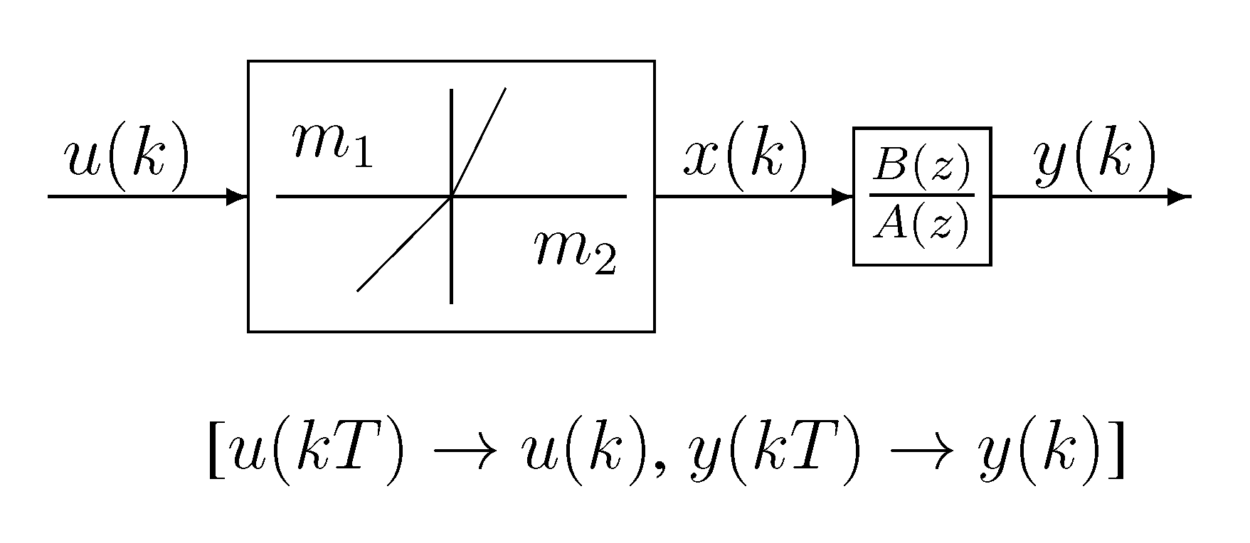
Assume that the corresponding discrete-time singe-rate Hammerstein system consists of a two-segment piecewise-linear nonlinearity with slopes $m_1$ and $m_2$ and a linear model with polynomials $A\left(z\right)$ and $B\left(z\right)$ as depicted in Figure 2,

$$\begin{array}{ccc}\hfill x\left(k\right)& =& \left\{\begin{array}{c}{m}_{1}u\left(k\right),u\left(k\right)\ge 0,\\ m_{2}u\left(k\right),u\left(k\right)<0,\end{array}\right.\hfill \end{array}$$

(1)

$$\begin{array}{ccc}\hfill A\left(z\right)y\left(k\right)& =& B\left(z\right)x\left(k\right),\hfill \end{array}$$

(2)

where $x\left(k\right)$ is the internal variable; $A\left(z\right)$ and $B\left(z\right)$ are defined by:

$$\begin{array}{ccc}\hfill A\left(z\right)& :=& 1+a_1{z}^{-1}+a_2{z}^{-2}+\cdots +a_n{z}^{-n},\hfill \end{array}$$

$$\begin{array}{ccc}\hfill B\left(z\right)& :=& b_0+b_1{z}^{-1}+b_2{z}^{-2}+\cdots +b_n{z}^{-n}.\hfill \end{array}$$

Figure 2. The discrete-time Hammerstein system.

Figure 2. The discrete-time Hammerstein system.

Introduce a switching function $h\left(k\right)$ as:

$$h\left(k\right)=h\left[u\right(k\left)\right]=0.5\{1+\text{sgn}[u\left(k\right)\left]\right\},$$

where:

$$\text{sgn}\left(u\right)=\left\{\begin{array}{cc}1,\hfill & u>0,\hfill \\ 0,\hfill & u=0,\hfill \\ -1,\hfill & u<0.\hfill \end{array}\right.$$

Then, Equation (1) can be rewritten as:

$$\begin{array}{c}\hfill x\left(k\right)=m_{2}u\left(k\right)+(m_1-m_2)h\left(k\right)u\left(k\right).\end{array}$$

(3)

From Equation (2), we have:

$$\begin{array}{c}\hfill y\left(k\right)=b_{0}x\left(k\right)+b_{1}x(k-1)+\cdots +b_{n}x(k-n)-a_{1}y(k-1)-a_{2}y(k-2)-\cdots -a_{n}y(k-n).\end{array}$$

(4)

Inserting Equation (3) into $x(k-i)$ in Equation (4) gives:

$$\begin{array}{c}\hfill y\left(k\right)=\sum _{i=0}^n{b}_i[m_{2}u(k-i)+(m_1-m_2)h(k-i)u(k-i)]-\sum _{i=1}^n{a}_{i}y(k-i).\end{array}$$

Define:

$$\begin{array}{ccc}\hfill U\left(k\right)& :=& \left[\begin{array}{c}u\left(k\right)h\left(k\right)u\left(k\right)\\ u(k-1)h(k-1)u(k-1)\\ ⋮\\ u(k-n)h(k-n)u(k-n)\end{array}\right]\in {ℝ}^{(n+1)\times 2},\hfill \\ \hfill \varphi \left(k\right)& :=& {[-y(k-1),-y(k-2),\cdots ,-y(k-n)]}^{\text{T}}\in {ℝ}^n,\hfill \\ \hfill \mathit{a}& :=& {[a_1,a_2,\cdots ,a_n]}^{\text{T}}\in {ℝ}^n,\hfill \\ \hfill \stackrel{-}{\mathit{b}}& :=& {[b_0,b_1,b_2,\cdots ,b_n]}^{\text{T}}\in {ℝ}^{n+1},\hfill \\ \hfill \mathit{M}& :=& {[m_2,m_1-m_2]}^{\text{T}}\in {ℝ}^2.\hfill \end{array}$$

Then, we have:

$$y\left(k\right)={\stackrel{-}{\mathit{b}}}^{\text{T}}\mathit{U}\left(k\right)\mathit{M}+{\varphi }^{\text{T}}\left(k\right)\mathit{a},$$

Replacing k with kq gives:

$$y\left(kq\right)={\stackrel{-}{\mathit{b}}}^{\text{T}}\mathit{U}\left(kq\right)\mathit{M}+{\varphi }^{\text{T}}\left(kq\right)\mathit{a},$$

(5)

The identification problems caused by dual-rate Hammerstein systems with piecewise-linear nonlinearity exist in two aspects.

• For the dual-rate Hammerstein system in this paper, all of the input data {u(k) : k = 0, 1, 2, …} are measurable; only a part of the output data {y(kq) : k = 0, 1, 2, …} can be measured, where q ≥ 2 is a positive integer. Intersample outputs (missing outputs) {y(kq − i) : k = 0, 1, 2, …, 0 < i < q} are unknown. Because there exist unavailable outputs y(kq − i) in the information vector ϕ(kq), with kq − i not equaling the integer multiples of q, the single-rate model in Equation (5) cannot be used as the identification model for the dual-rate system.
• Moreover, the single-rate model in Equation (5) contains the products of the parameters of the nonlinear block and the linear block, i.e., the output of the model is a bilinear function about the parameter vectors $\stackrel{-}{\mathit{b}}$ and M, and a standard least squares method cannot be directly applied to the model.

The intent of this paper is to convert the Hammerstein system in Equations (1) and (2) into a dual-rate linear regression model about all parameters (linear-in-parameter model), by combining the polynomial transformation technique [20] with the key variable separation technique [12]. The obtained dual-rate linear regression model is suitable for the dual-rate sampled data, and a standard identification technique can be directly applied to the model to estimate the parameters of the model.

3. The Dual-Rate Identification Model of the Hammerstein System

In this section, we transform the Hammerstein system in Equations (1) and (2) into a dual-rate linear-in-parameter identification model, which is suitable for the dual-rate sampled data, by using the polynomial transformation technique [20] and the key variable separation technique [12].

Referring to [20], assume that the roots of $A\left(z\right)$ are $z_i,i=1,2,\cdots ,n$. Then, we have:

$$\begin{array}{c}\hfill A\left(z\right)=(1-z_1{z}^{-1})(1-z_2{z}^{-1})\cdots (1-z_n{z}^{-1}).\end{array}$$

Define:

$$\begin{array}{ccc}\hfill ϵ\left(z\right)& :=& (1+z_1{z}^{-1}+z_1^2{z}^{-2}+\cdots +z_1^{q-1}{z}^{-q+1})(1+z_2{z}^{-1}+z_2^2{z}^{-2}+\cdots +z_2^{q-1}{z}^{-q+1})\cdots \hfill \\ & & (1+z_n{z}^{-1}+z_n^2{z}^{-2}+\cdots +z_n^{q-1}{z}^{-q+1})\hfill \\ & =& 1+{ϵ}_1{z}^{-1}+{ϵ}_2{z}^{-2}+\cdots +{ϵ}_{n(q-1)}{z}^{-n(q-1)}.\hfill \end{array}$$

Multiplying both sides of Equation (2) by $ϵ\left(z\right)$ gives:

$$\alpha \left(z\right)y\left(k\right)=\beta \left(z\right)x\left(k\right).$$

Using the identity:

$$1-z_i^q{z}^{-q}\equiv (1-z_i{z}^{-1})(1+z_i{z}^{-1}+z_i^2{z}^{-2}+\cdots +z_i^{q-1}{z}^{-(q-1)}),$$

one obtains:

$$\begin{array}{ccc}\hfill \alpha \left(z\right)& :=& ϵ\left(z\right)A\left(z\right)\hfill \\ & =& (1+z_1{z}^{-1}+z_1^2{z}^{-2}+\cdots +z_1^{q-1}{z}^{-(q-1)})(1-z_1{z}^{-1})\hfill \\ & & (1+z_2{z}^{-1}+z_2^2{z}^{-2}+\cdots +z_2^{q-1}{z}^{-(q-1)})(1-z_2{z}^{-1})\hfill \\ & & \cdots \hfill \\ & & (1+z_n{z}^{-1}+z_n^2{z}^{-2}+\cdots +z_n^{q-1}{z}^{-(q-1)})(1-z_n{z}^{-1})\hfill \\ & =& (1-z_1^q{z}^{-q})(1-z_2^q{z}^{-q})\cdots (1-z_n^q{z}^{-q})\hfill \\ & =:& 1+{\alpha }_1{z}^{-q}+{\alpha }_2{z}^{-2q}+\cdots +{\alpha }_n{z}^{-nq},\hfill \end{array}$$

(6)

$$\begin{array}{ccc}\hfill \beta \left(z\right)& :=& ϵ\left(z\right)B\left(z\right)\hfill \\ & =& (1+{ϵ}_1{z}^{-1}+{ϵ}_2{z}^{-2}+\cdots +{ϵ}_{n(q-1)}{z}^{-n(q-1)})(b_0+b_1{z}^{-1}+b_2{z}^{-2}+\cdots +b_n{z}^{-n})\hfill \\ & =:& {\beta }_0+{\beta }_1{z}^{-1}+{\beta }_2{z}^{-2}+\cdots +{\beta }_{nq}{z}^{-nq}.\hfill \end{array}$$

(7)

Consider a disturbance in a practical system; introducing a zero-mean random white noise $v\left(k\right)$, we have:

$$\begin{array}{c}\hfill \alpha \left(z\right)y\left(k\right)=\beta \left(z\right)x\left(k\right)+v\left(k\right).\end{array}$$

(8)

Substituting the polynomials $\alpha \left(z\right)$ and $\beta \left(z\right)$ into Equation (8) gives:

$$\begin{array}{ccc}\hfill y\left(k\right)& =& [{\beta }_0+{\beta }_1{z}^{-1}+{\beta }_2{z}^{-2}+\cdots +{\beta }_{nq}{z}^{-nq}]x\left(k\right)\hfill \\ & & -[{\alpha }_1{z}^{-q}+{\alpha }_2{z}^{-2q}+\cdots +{\alpha }_n{z}^{-nq}]y\left(k\right)+v\left(k\right),\hfill \end{array}$$

(9)

$$\begin{array}{ccc}& =& {\beta }_{0}x\left(k\right)+\sum _{i=1}^{nq}{\beta }_{i}x(k-i)-\sum _{i=1}^n{\alpha }_{i}y(k-iq)+v\left(k\right).\hfill \end{array}$$

(10)

In order to get a unique solution, we assume that ${\beta }_0=b_0=1$ [21]. The first term $x\left(k\right)$ (its coefficient is one) on the right-hand side is a separated key variable, and $x(k-i)(i=1,2,\cdots ,n_{\beta })$ are not separated variables. Substituting (3) into the separated key variable $x\left(k\right)$ in Equation (10) gives:

$$\begin{array}{c}\hfill y\left(k\right)=m_{2}u\left(k\right)+(m_1-m_2)h\left(k\right)u\left(k\right)+\sum _{i=1}^{nq}{\beta }_{i}x(k-i)-\sum _{i=1}^n{\alpha }_{i}y(k-iq)+v\left(k\right).\end{array}$$

Define the information vector $\psi \left(k\right)$ and the parameter vector Θ as:

$$\begin{array}{ccc}\hfill \psi \left(k\right)& :=& \left[u\right(k),h(k\left)u\right(k),x(k-1),x(k-2),\cdots ,x(k-nq),-y(k-q),-y(k-2q),\cdots ,\hfill \\ & & {-y(t-nq)]}^{\text{T}}\in {ℝ}^{nq+n+2},\hfill \\ \hfill \Theta & :=& {[m_2,m_1-m_2,{\beta }_1,{\beta }_2,\cdots ,{\beta }_{nq},{\alpha }_1,{\alpha }_2,\cdots ,{\alpha }_n]}^{\text{T}}\in {ℝ}^{nq+n+2}.\hfill \end{array}$$

Then, we have:

$$y\left(k\right)={\psi }^{\text{T}}\left(k\right)\Theta +v\left(k\right).$$

Replacing k with kq gives the following dual-rate linear-in-parameter identification model,

$$y\left(kq\right)={\psi }^{\text{T}}\left(kq\right)\Theta +v\left(kq\right),$$

(11)

with:

$$\begin{array}{ccc}\hfill \psi \left(kq\right)& :=& {\left[u\right(kq),h(kq\left)u\right(kq),x(kq-1),x(kq-2),\cdots ,x(kq-nq),-y(kq-q),-y(kq-2q),\cdots ,-y(kq-nq\left)\right]}^{\text{T}}\hfill \end{array}$$

(12)

The output of the obtained model is linear about all parameters. Note that y(kq − iq) is available by sampling the output signal in every qT interval, and y(kq) in Equation (11) is a linear function about Θ. Thus, it is easy to estimate the parameter vector Θ by using the standard least squares method.

4. The Dual-Rate/Single-Rate Parameter Estimation

In this section, the parameter estimates (in the following $\widehat{\Theta }\left(kq\right)$) of the dual-rate model are computed by a recursive least squares algorithm; then by comparing the coefficients of $z^{-i}$ on both sides of a coefficient polynomial equation containing the parameters of the dual-rate/single-rate models, the parameter estimates (in the following $\widehat{\theta }\left(kq\right)$) of the single-rate model are derived.

Suppose that the data length $N\gg nq+n+2$. Define a quadratic cost function,

$$J(\Theta ):=\sum _{k=1}^N{[y\left(kq\right)-{\psi }^{\text{T}}\left(kq\right)\Theta ]}^2.$$

The information vector $\psi \left(kq\right)$ in $J\left(\Theta \right)$ contains the unknown internal variables $\left\{x\right(kq-i),i=1,2,\cdots ,nq\}$. Here, the solution is to replace $x(kq-i)$ with its estimate $\widehat{x}(kq-i)$; then the estimate of $\psi \left(kq\right)$ can be written as:

$$\begin{array}{ccc}\hfill \widehat{\psi }\left(kq\right)& :=& {[u\left(kq\right),h\left(kq\right)u\left(kq\right),\widehat{x}(kq-1),\widehat{x}(kq-2),\cdots ,\widehat{x}(kq-nq),-y(kq-q),-y(kq-2q),\cdots ,-y(kq-nq)]}^{\text{T}}.\hfill \end{array}$$

(13)

the estimate $\widehat{x}(kq-i)$ can be computed by replacing m₁ and m₂ in Equation (3) with their estimates ${\widehat{m}}_1\left(kq\right)$ and ${\widehat{m}}_2\left(kq\right)$,

$$\widehat{x}(kq-i)={\widehat{m}}_2\left(kq\right)u(kq-i)+[{\widehat{m}}_1\left(kq\right)-{\widehat{m}}_2\left(kq\right)]h(kq-i)u(kq-i).$$

Minimizing the cost functions $J(\Theta )$, replacing $x(kq-i)$ in $\psi \left(kq\right)$ with its estimate $\widehat{x}(kq-i)$ and by using the least squares method, we obtain the following key variable separation-based recursive least squares algorithm for estimating Θ of the dual-rate Hammerstein system,

$$\begin{array}{ccc}\hfill \widehat{\Theta }\left(kq\right)& =& \widehat{\Theta }(kq-q)+\mathit{L}\left(kq\right)[y\left(kq\right)-{\widehat{\psi }}^{\text{T}}\left(kq\right)\widehat{\Theta }(kq-q)],\hfill \end{array}$$

(14)

$$\begin{array}{ccc}\hfill \mathit{L}\left(kq\right)& =& \frac{\mathit{P}(kq-q)\widehat{\psi }\left(kq\right)}{1+{\widehat{\psi }}^{\text{T}}\left(kq\right)\mathit{P}(kq-q)\widehat{\psi }\left(kq\right)},\hfill \end{array}$$

(15)

$$\begin{array}{ccc}\hfill \mathit{P}\left(kq\right)& =& [\mathit{I}-\mathit{L}\left(kq\right){\widehat{\psi }}^{\text{T}}\left(kq\right)]\mathit{P}(kq-q),\mathit{P}\left(0\right)=p_0\mathit{I},\hfill \end{array}$$

(16)

$$\begin{array}{ccc}\hfill \widehat{\psi }\left(kq\right)& =& {[u\left(kq\right),h\left(kq\right)u\left(kq\right),\widehat{x}(kq-1),\widehat{x}(kq-2),\cdots ,\widehat{x}(kq-nq),-y(kq-q),-y(kq-2q),\cdots ,-y(kq-nq)]}^{\text{T}},\hfill \end{array}$$

(17)

$$\widehat{x}(kq+i)={\widehat{m}}_2\left(kq\right)u(kq+i)+[{\widehat{m}}_1\left(kq\right)-{\widehat{m}}_2\left(kq\right)]h(kq+i)u(kq+i),$$

(18)

$$\widehat{\Theta }\left(kq\right)=[{\widehat{m}}_2\left(kq\right),{\widehat{m}}_1\left(kq\right)-{\widehat{m}}_2\left(kq\right),{\widehat{\beta }}_1\left(kq\right),{\widehat{\beta }}_2\left(kq\right),\cdots ,{\widehat{\beta }}_{nq}\left(kq\right),{\widehat{\alpha }}_1\left(kq\right),{\widehat{\alpha }}_2\left(kq\right),\cdots ,{\widehat{\beta }}_n\left(kq\right){]}^{\text{T}}.$$

(19)

Use the obtained $\widehat{\Theta }\left(kq\right)$ to construct the polynomials,

$$\widehat{\alpha }(kq,z)=1+{\widehat{\alpha }}_1\left(kq\right)z^{-q}+{\widehat{\alpha }}_2\left(kq\right)z^{-2q}+\cdots +{\widehat{\alpha }}_n\left(kq\right)z^{-nq},$$

$$\widehat{\text{β}}(kq,z)=1+{\widehat{\beta }}_1\left(kq\right)z^{-q}+{\widehat{\beta }}_2\left(kq\right)z^{-2q}+\cdots +{\widehat{\beta }}_n\left(kq\right)z^{-nq}.$$

From Equations (6) and (7), we can get:

$$\frac{\alpha \left(z\right)}{\beta \left(z\right)}=\frac{A\left(z\right)}{B\left(z\right)}.$$

Let the estimates of A(z) and B(z) at time kq be:

$$\widehat{A}(kq,z)=1+{\widehat{a}}_1\left(kq\right)z^{-1}+{\widehat{a}}_2\left(kq\right)z^{-2}+\cdots +{\widehat{a}}_n\left(kq\right)z^{-n},$$

$$\widehat{B}(kq,z)=1+{\widehat{b}}_1\left(kq\right)z^{-1}+{\widehat{b}}_2\left(kq\right)z^{-2}+\cdots +{\widehat{b}}_n\left(kq\right)z^{-n}.$$

According to the model equivalence principle, let:

$$\frac{\widehat{\alpha }(kq,z)}{\widehat{\text{β}}(kq,z)}=\frac{\widehat{A}(kq,z)}{\widehat{B}(kq,z)},$$

then we have

$$\widehat{\alpha }(kq,z)\widehat{B}(kq,z)=\widehat{\beta }(kq,z)\widehat{A}(kq,z),$$

By comparing the coefficients of $z^{-i}$ on both sides of this equation, we can establish a series of linear equations about ${\widehat{a}}_i\left(kq\right)$ and ${\widehat{b}}_i\left(kq\right)$ and build a matrix equation as:

$$\begin{array}{c}\hfill \mathit{T}\left(kq\right)\widehat{\mathit{\theta }}\left(kq\right)=\mathit{\rho }\left(kq\right),\end{array}$$

(20)

where:

$$\begin{array}{ccc}\hfill \widehat{\mathit{\theta }}\left(kq\right)& =& {[{\widehat{a}}_1\left(kq\right),{\widehat{a}}_2\left(kq\right),\cdots ,{\widehat{a}}_n\left(kq\right),{\widehat{b}}_1\left(kq\right),{\widehat{b}}_2\left(kq\right),\cdots ,{\widehat{b}}_n\left(kq\right)]}^{\text{T}}\in {ℝ}^{2n},\hfill \end{array}$$

$$\begin{array}{ccc}\hfill \mathit{\rho }\left(kq\right)& =& {[{\widehat{\beta }}_1\left(kq\right)-{\lambda }_1\left(kq\right),{\widehat{\beta }}_2\left(kq\right)-{\lambda }_2\left(kq\right),\cdots ,{\widehat{\beta }}_{nq}\left(kq\right)-{\lambda }_{nq}\left(kq\right),0,\cdots ,0]}^{\text{T}}\in {ℝ}^{nq+n},\hfill \end{array}$$

(21)

$$\begin{array}{ccc}\hfill \mathit{T}\left(kq\right)& =& -{\mathit{T}}_{\text{β}}\left(kq\right){\mathit{T}}_{\alpha }\left(kq\right)]\in {ℝ}^{(nq+n)·2n},\hfill \end{array}$$

(22)

$$\begin{array}{c}\hfill {\mathit{T}}_{\alpha }\left(kq\right)=\left[\begin{array}{cccc}1& 0& \cdots & 0\\ {\lambda }_1\left(kq\right)& 1& & ⋮\\ {\lambda }_2\left(kq\right)& {\lambda }_1\left(kq\right)& \ddots & 0\\ ⋮& {\lambda }_2\left(kq\right)& \ddots & 1\\ ⋮& & \ddots & {\lambda }_1\left(kq\right)\\ {\lambda }_{nq}\left(kq\right)& & & {\lambda }_2\left(kq\right)\\ 0& {\lambda }_{nq}\left(kq\right)& & ⋮\\ ⋮& & \ddots & ⋮\\ 0& \cdots & & {\lambda }_{nq}\left(kq\right)\end{array}\right]\in {ℝ}^{(nq+n)\times n},\end{array}$$

(23)

$$\begin{array}{c}\hfill {\lambda }_i\left(kq\right)=\left\{\begin{array}{c}{\widehat{\alpha }}_j\left(kq\right),i=jq,j=1,2,\cdots ,n,\hfill \\ 0,others,\hfill \end{array}\right.\end{array}$$

(24)

$$\begin{array}{c}\hfill {\mathit{T}}_{\text{β}}\left(kq\right)=\left[\begin{array}{cccc}1& 0& \cdots & 0\\ {\widehat{\beta }}_1\left(kq\right)& 1& & 0\\ {\widehat{\beta }}_2\left(kq\right)& {\widehat{\beta }}_1\left(kq\right)& & ⋮\\ ⋮& {\widehat{\beta }}_2\left(kq\right)& \ddots & 1\\ ⋮& & \ddots & {\widehat{\beta }}_1\left(kq\right)\\ {\widehat{\text{β}}}_{nq}\left(kq\right)& & & {\widehat{\beta }}_2\left(kq\right)\\ 0& {\widehat{\beta }}_{nq}\left(kq\right)& & ⋮\\ ⋮& & \ddots & ⋮\\ 0& \cdots & 0& {\widehat{\beta }}_{nq}\left(kq\right)\end{array}\right]\in {ℝ}^{(nq+n)\times n}.\end{array}$$

(25)

Then, the least squares solution for Equation (20) is given by:

$$\widehat{\theta }\left(kq\right)={\left[{\mathit{T}}^{\text{T}}\right(kq\left)\mathit{T}\right(kq\left)\right[}^{-1}{\mathit{T}}^{\text{T}}\left(kq\right)\mathit{\rho }\left(kq\right).$$

(26)

The computation process for estimates $\widehat{\Theta }\left(kq\right)$ and $\widehat{\theta }\left(kq\right)$ of the key variable separation-based recursive least squares algorithm for the dual-rate Hammerstein system is summarized as follows:

• Step 1. To initialize, let k = 1 and $\widehat{\Theta }$ (0) = 1_nq+n+2/p0, and P(0) = p₀I, $\widehat{x}$(kq) = 0; u(k) = 0; y(k) = 0, for k ≤ 0, p₀ = 10⁶.
• Step 2. Collect the input-output data u(k) and y(kq), and form $\widehat{\psi }\left(kq\right)$ by Equation (17).
• Step 3. Compute L(kq) by Equation (15) and P(kq) by Equation (16).
• Step 4. Update the dual-rate parameter estimate $\widehat{\Theta }\left(kq\right)$ by Equation (14).
• Step 5. Compute $\widehat{x}(kq+i)$ by Equation (18).
• Step 6. Form $\rho \left(kq\right)$, ${\mathit{T}}_{\alpha }\left(kq\right)$, ${\mathit{T}}_{\text{β}}\left(kq\right)$ and $\mathit{T}\left(kq\right)$ by Equation (21), Equation (23), Equation (25) and Equation (22).
• Step 7. Update the single-rate parameter estimate $\widehat{\theta }\left(kq\right)$ by Equation (26).
• Step 8. Increase k by one and go to Step 2.

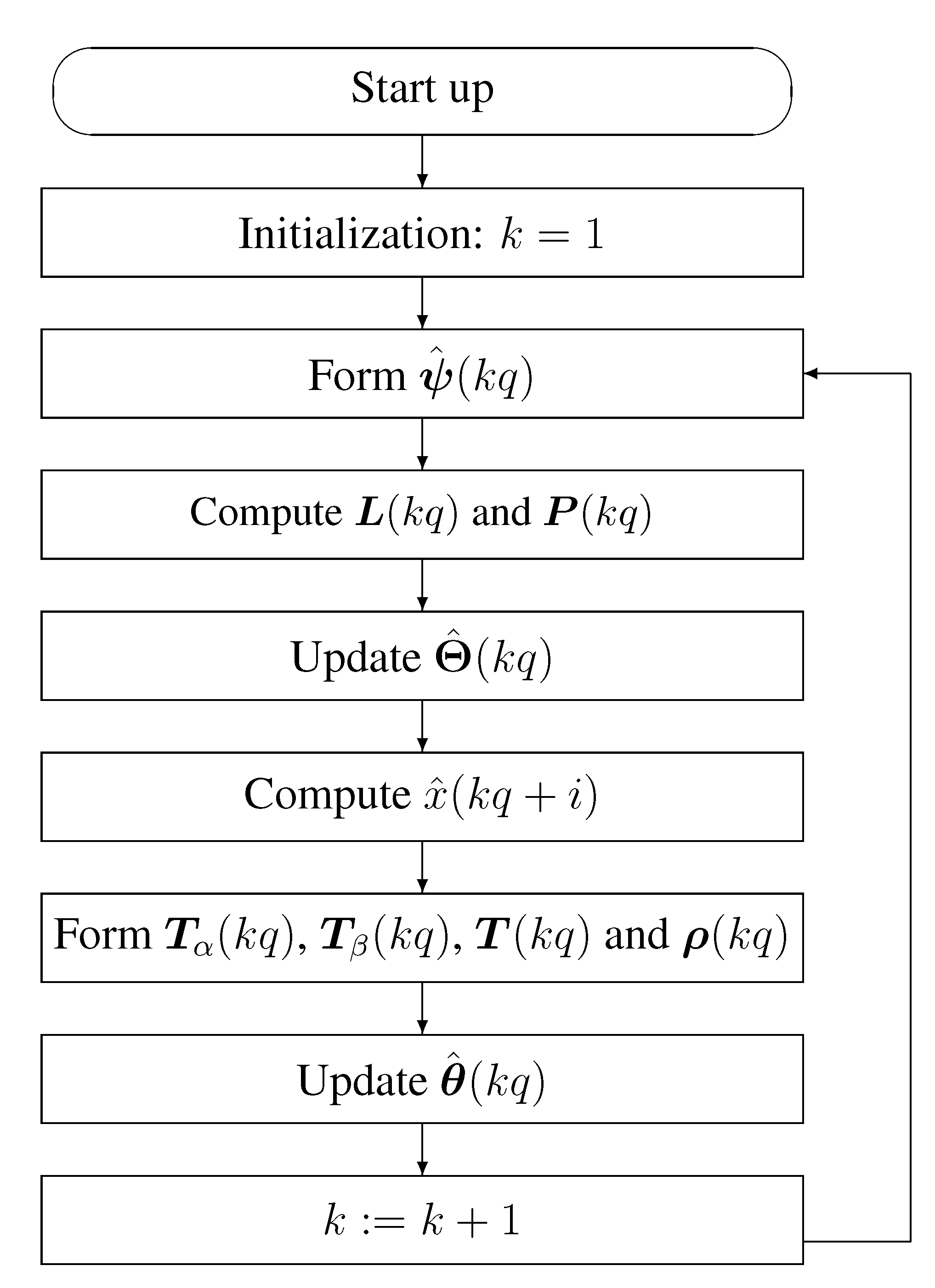
The procedure of computing the estimates $\widehat{\Theta }\left(kq\right)$ and $\widehat{\theta }\left(kq\right)$ of the key variable separation-based recursive least squares algorithm is shown in Figure 3.

Figure 3. The flowchart for computing the estimates $\widehat{\Theta }\left(kq\right)$ and $\widehat{\theta }\left(kq\right)$.

Figure 3. The flowchart for computing the estimates $\widehat{\Theta }\left(kq\right)$ and $\widehat{\theta }\left(kq\right)$.

5. The Convergence Analysis

The convergence analysis of the presented key variable separation-based recursive least squares algorithm for a dual-rate Hammerstein system is simply explained as follows.

Assume that the σ algebra sequence ${Ƒ}_{kq}=\sigma (v\left(kq\right),v(kq-1),v(kq-2),\cdots )$ generated by $v\left(kq\right)$, and $\{v\left(kq\right),{Ƒ}_{kq}\}$ is a martingale difference sequence on a probability space $\left\{\text{Ω},Ƒ,P\right\}$ [22]. The sequence $\left\{v\right(kq\left)\right\}$ satisfies:

$$\begin{array}{ccc}\hfill \left(A1\right)& & \text{E}\left[v\left(kq\right)\right|{Ƒ}_{kq-q}]=0,\text{a.s.}\hfill \\ \hfill \left(A2\right)& & \text{E}\left[v^2\left(kq\right)\right|{Ƒ}_{kq-q}]={\sigma }^2\left(kq\right)⩽{\overline{\sigma }}^2<\infty ,\text{a.s.}\hfill \\ \hfill \left(A3\right)& & \underset{t\to \infty }{lim\; sup}\frac{1}{t}\sum _{i=q}^{kq}{v}^2\left(i\right)⩽{\overline{\sigma }}^2<\infty ,\text{a.s.}\hfill \end{array}$$

Theorem 1: For the key variable separation-based recursive least squares algorithm in this paper, assume that (A1)–(A3) hold and that the estimated information vector $\widehat{\psi }\left(kq\right)$ and matrix $\mathit{T}\left(kq\right)$ are persistently exciting, i.e., there exist constants $0<C_1\le C_2<\infty$ and an integer $N>n_0(n_0=nq+n+2)$, such that for $k>n_0$, the following strong persistent excitation conditions hold:

$$\begin{array}{ccc}\hfill \left(A4\right)& & C_1\mathit{I}⩽\frac{1}{N}\sum _{k=0}^{N-1}\widehat{\psi }\left(kq\right){\widehat{\psi }}^{\text{T}}\left(kq\right)⩽C_2\mathit{I},\text{a.s.}\hfill \end{array}$$

$$\begin{array}{ccc}\hfill \left(A5\right)& & C_1\mathit{I}⩽\frac{1}{N}\sum _{k=0}^{N-1}{\mathit{T}}^{\text{T}}\left(kq\right)\text{T}\left(kq\right)⩽C_2\mathit{I},\text{a.s.}\hfill \end{array}$$

Then, the parameter estimation vectors $\widehat{\Theta }\left(kq\right)$ and $\widehat{\theta }\left(kq\right)$ consistently converge to the true parameter vectors Θ and θ.

In a similar way to the method in [23], Theorem 1 can be proven, and its proof is omitted here.

6. Experiment

Consider the following Hammerstein system:

$$\begin{array}{ccc}\hfill A\left(z\right)y\left(k\right)& =& B\left(z\right)x\left(k\right)+v\left(k\right),\hfill \\ \hfill x\left(k\right)& =& \left\{\begin{array}{c}{m}_{1}u\left(k\right)u\left(k\right)\ge 0\hfill \\ m_{2}u\left(k\right)u\left(k\right)<0\hfill \end{array}\right.,\hfill \\ \hfill A\left(z\right)& =& 1+a_1{z}^{-1}+a_2{z}^{-2}\hfill \\ & =& 1+0.20z^{-1}-0.35z^{-2},\hfill \\ \hfill B\left(z\right)& =& 1+b_1{z}^{-1}+b_2{z}^{-2}\hfill \\ & =& 1+0.80z^{-1}+0.60z^{-2},\hfill \\ \hfill m_1& =& 1.50,m_2=-1.00.\hfill \end{array}$$

Suppose $q=2$; then, we have:

$$\epsilon \left(z\right)=1-0.20z^{-1}-0.35z^{-2}.$$

The corresponding dual-rate model can be expressed as:

$$\begin{array}{ccc}\hfill \alpha \left(z\right)y\left(k\right)& =& \beta \left(z\right)x\left(k\right),\hfill \\ \hfill \alpha \left(z\right)& =& 1+{\alpha }_1{z}^{-2}+{\alpha }_2{z}^{-4}\hfill \\ & =& 1-0.74z^{-2}+0.1225z^{-4},\hfill \\ \hfill \text{β}\left(z\right)& =& 1+{\beta }_1{z}^{-1}+{\beta }_2{z}^{-2}+{\beta }_3{z}^{-3}+{\beta }_4{z}^{-4}\hfill \\ & =& 1+0.60z^{-1}+0.09z^{-2}-0.40z^{-3}-0.21z^{-4},\hfill \\ \mathit{a}& =& {[0.20,-0.35]}^{\text{T}},\mathit{b}={[0.80,0.60]}^{\text{T}},\hfill \\ \mathit{\theta }& =& \left[\begin{array}{c}\mathit{a}\\ \mathit{b}\end{array}\right],\hfill \\ \mathit{\alpha }& =& {[-0.74,0.1225]}^{\text{T}},\mathit{\beta }={[0.69,0.09,-0.40,-0.21]}^{\text{T}},\hfill \\ \Theta & =& {[m_2,m_1-m_2,{\text{β}}^{\text{T}},{\alpha }^{\text{T}}]}^{\text{T}}.\hfill \end{array}$$

In the simulation experiment, the input {u(t)} is taken as an uncorrelated persistently-excited normal distribution signal sequence with zero mean and unit variance, and {v(t)} is taken as a white noise sequence with zero mean and variance σ² = 0.50² and σ² = 1.00². Apply the proposed algorithm to estimate the parameters of this system. The parameter estimation errors of the dual-rate model are:

$$\delta :=\sqrt{\frac{\parallel {\widehat{m}}_1\left(kq\right)-m_1{\parallel }^2+\parallel {\widehat{m}}_2\left(kq\right)-m_2{\parallel }^2+\parallel \widehat{\text{β}}{\left(kq\right)-\text{β}\parallel }^2+{\parallel \widehat{\alpha }\left(kq\right)-\alpha \parallel }^2}{m_1^2+m_2^2+{\parallel \text{β}\parallel }^2+{\parallel \alpha \parallel }^2}}\times 100\%,$$

the parameter estimation errors of the single-rate model are:

$$\delta :=\sqrt{\frac{\parallel {\widehat{m}}_1\left(kq\right)-m_1{\parallel }^2+\parallel {\widehat{m}}_2\left(kq\right)-m_2{\parallel }^2+\parallel \widehat{a}{\left(kq\right)-a\parallel }^2+{\parallel \widehat{b}\left(kq\right)-b\parallel }^2}{m_1^2+m_2^2+{\parallel a\parallel }^2+{\parallel b\parallel }^2}}\times 100\%,$$

The parameter estimates and their errors are shown in Table 1 and Table 2. Obviously, the parameter estimation errors become (generally) smaller and smaller with the data length k increasing. This shows that the proposed algorithm is effective.

Table 1. The single-rate parameter estimates and errors.

σ2	0.502				1.002
t	100	1000	2000	3000	100	1000	2000	3000
$m_1$= 1.5000	1.64510	1.49306	1.48069	1.48674	1.64332	1.47369	1.45489	1.46773
$m_2$=−1.0000	−1.10137	−1.00671	−0.98836	−0.99494	−1.07085	−0.98956	−0.96557	−0.98115
${\text{β}}_1$= 0.6000	0.44924	0.56619	0.58761	0.60112	0.46040	0.54639	0.58138	0.60706
${\text{β}}_2$= 0.0900	−0.02088	0.04436	0.07612	0.08695	−0.07241	0.04529	0.09448	0.10813
${\text{β}}_3$= −0.4000	−0.10421	−0.33348	−0.35710	−0.36657	−0.13676	−0.33817	−0.35584	−0.36336
${\text{β}}_4$= −0.2100	−0.16787	−0.18590	−0.20263	−0.20855	−0.14399	−0.16044	−0.19223	−0.20651
${\alpha }_1$=−0.7400	−0.70650	−0.75683	−0.74221	−0.73669	−0.77498	−0.75709	−0.72961	−0.72063
${\alpha }_2$= 0.1225	0.15543	0.14357	0.12683	0.12660	0.18953	0.13963	0.11305	0.11506
$\delta (\%)$=0.0000	18.97213	4.54356	2.51473	1.76071	18.54456	5.34749	3.71454	2.84976

Table 1. The single-rate parameter estimates and errors.

σ2	0.502				1.002
t	100	1000	2000	3000	100	1000	2000	3000
$m_1$= 1.5000	1.64510	1.49306	1.48069	1.48674	1.64332	1.47369	1.45489	1.46773
$m_2$=−1.0000	−1.10137	−1.00671	−0.98836	−0.99494	−1.07085	−0.98956	−0.96557	−0.98115
${\text{β}}_1$= 0.6000	0.44924	0.56619	0.58761	0.60112	0.46040	0.54639	0.58138	0.60706
${\text{β}}_2$= 0.0900	−0.02088	0.04436	0.07612	0.08695	−0.07241	0.04529	0.09448	0.10813
${\text{β}}_3$= −0.4000	−0.10421	−0.33348	−0.35710	−0.36657	−0.13676	−0.33817	−0.35584	−0.36336
${\text{β}}_4$= −0.2100	−0.16787	−0.18590	−0.20263	−0.20855	−0.14399	−0.16044	−0.19223	−0.20651
${\alpha }_1$=−0.7400	−0.70650	−0.75683	−0.74221	−0.73669	−0.77498	−0.75709	−0.72961	−0.72063
${\alpha }_2$= 0.1225	0.15543	0.14357	0.12683	0.12660	0.18953	0.13963	0.11305	0.11506
$\delta (\%)$=0.0000	18.97213	4.54356	2.51473	1.76071	18.54456	5.34749	3.71454	2.84976

Table 2. The single-rate parameter estimates and errors.

σ2	0.502				1.002
t	100	1000	2000	3000	100	1000	2000	3000
$m_1$= 1.5000	1.64332	1.47369	1.45489	1.46773	1.64510	1.49306	1.48069	1.48674
$m_2$=−1.0000	−1.07085	−0.98956	−0.96557	−0.98115	−1.10137	−1.00671	−0.98836	−0.99494
$a_1$= 0.2000	−0.13036	0.18131	0.18225	0.16469	−0.16282	0.13686	0.15786	0.15793
$a_2$=−0.3500	−0.28358	−0.40123	−0.36730	−0.34446	−0.21271	−0.36634	−0.35419	−0.34545
$b_1$= 0.8000	0.33046	0.72731	0.76196	0.77122	0.28415	0.70397	0.74542	0.75947
$b_2$= 0.6000	0.36387	0.50014	0.56053	0.58345	0.40609	0.51357	0.55673	0.57349
$\delta (\%)$=0.0000	30.68012	6.56738	3.93705	2.92556	33.17133	6.90524	4.02630	3.13498

Table 2. The single-rate parameter estimates and errors.

σ2	0.502				1.002
t	100	1000	2000	3000	100	1000	2000	3000
$m_1$= 1.5000	1.64332	1.47369	1.45489	1.46773	1.64510	1.49306	1.48069	1.48674
$m_2$=−1.0000	−1.07085	−0.98956	−0.96557	−0.98115	−1.10137	−1.00671	−0.98836	−0.99494
$a_1$= 0.2000	−0.13036	0.18131	0.18225	0.16469	−0.16282	0.13686	0.15786	0.15793
$a_2$=−0.3500	−0.28358	−0.40123	−0.36730	−0.34446	−0.21271	−0.36634	−0.35419	−0.34545
$b_1$= 0.8000	0.33046	0.72731	0.76196	0.77122	0.28415	0.70397	0.74542	0.75947
$b_2$= 0.6000	0.36387	0.50014	0.56053	0.58345	0.40609	0.51357	0.55673	0.57349
$\delta (\%)$=0.0000	30.68012	6.56738	3.93705	2.92556	33.17133	6.90524	4.02630	3.13498

7. Conclusions

The solution to overcoming the identification difficulties of the dual-rate Hammerstein system is to derive a dual-rate identification model that must be suitable for the dual-rate sampled data, and it is easy to use a standard least squares method. By combining the polynomial transformation technique with the key variable separation technique, this paper converts the discrete-time Hammerstein system into a dual-rate linear regression model about all parameters, which is suitable for the dual-rate sampled data and presents a recursive least squares algorithm for the dual-rate linear-in-parameter model to get the parameters of the dual-rate model. Finally, the parameters of the single-rate model are computed by a least squares algorithm from the obtained parameters of the dual-rate model. The proposed method can be used in the soft measurement of dual-rate nonlinear systems.

References

1. Igbida, N.; Karami, F.; Ta, T.N.N. Discrete collapsing sandpile model. Nonlinear Anal. 2014, 99, 177–189. [Google Scholar] [CrossRef]
2. Zaslavski, A.J. Stability of a turnpike phenomenon for approximate solutions of nonautonomous discrete-time optimal control systems. Nonlinear Anal. 2014, 100, 1–22. [Google Scholar] [CrossRef]
3. Chen, J.; Lv, L.X.; Ding, R.F. Multi-innovation stochastic gradient algorithms for dual-rate sampled systems with preload nonlinearity. Appl. Math. Lett. 2013, 26, 124–129. [Google Scholar] [CrossRef]
4. Chen, J. Several gradient parameter estimation algorithms for dual-rate sampled systems. J. Frankl. Inst. 2014, 351, 543–554. [Google Scholar] [CrossRef]
5. Kumbasar, E.P.A.; Aydin, H.; Ondogan, Z.; Ozcelik, M.; Ondogan, E.N. Automatic indigo measurement system as part of a dosing system for indigo Dyeing. Fibres Text. East. Eur. 2006, 14, 86–90. [Google Scholar]
6. Ding, J.; Ding, F.; Liu, X.P.; Liu, G. Hierarchical least squares identification for linear SISO systems with dual-rate sampled-data. IEEE Trans. Automat. Control 2011, 56, 2677–2683. [Google Scholar] [CrossRef]
7. Liu, Y.J.; Ding, F.; Shi, Y. An efficient hierarchical identification method for general dual-rate sampled-data systems. Automatica 2014, 50, 962–973. [Google Scholar] [CrossRef]
8. Huang, J.; Shi, Y.; Huang, H.N.; Li, Z. l2-l filtering for multirate nonlinear sampled-data systems using T-S fuzzy models. Digit. Signal Proc. 2013, 23, 418–426. [Google Scholar] [CrossRef]
9. Haber, R.; Keviczky, L. Nonlinear System Identification-Input-Output Modeling Approach; Kluwer Academic Publishers: Dorchrecht, The Netherlands; Boston, MA, USA; London, UK, 1999. [Google Scholar]
10. Vörös, J. Parameter identification of Wiener systems with multisegment piecewise-linear nonlinearities. Syst. Control Lett. 2007, 56, 99–105. [Google Scholar] [CrossRef]
11. Chidambaram, M. Computer Control of Processes; CRC Press: New York, NY, USA, 2001. [Google Scholar]
12. Wang, D.Q.; Chu, Y.Y.; Yang, G.W.; Ding, F. Auxiliary model-based recursive generalized least squares parameter estimation for Hammerstein OEAR systems. Math. Comput. Model. 2010, 52, 309–317. [Google Scholar] [CrossRef]
13. Vörös, J. Iterative algorithm for parameter identification of Hammerstein systems with two-segment nonlinearities. IEEE Trans. Automat. Control 1999, 44, 2145–2149. [Google Scholar] [CrossRef]
14. Vörös, J. Identification of Hammerstein systems with time-varying piecewise-linear chatacteristics. IEEE Trans. Circuits Syst. II 2005, 52, 865–869. [Google Scholar] [CrossRef]
15. Vörös, J. Identification of nonlinear cascade systems with time-varying backlash. J. Electr. Eng. 2011, 62, 87–92. [Google Scholar] [CrossRef]
16. Deng, K.P.; Ding, F. Newton iterative identification method for an input nonlinear finite impulse response system with moving average noise using the key variables separation technique. Nonlinear Dyn. 2014, 76, 1195–1202. [Google Scholar] [CrossRef]
17. Li, J.H. Parameter estimation for Hammerstein CARARMA systems based on the Newton iteration. Appl. Math. Lett. 2013, 26, 91–96. [Google Scholar] [CrossRef]
18. Wang, C.; Tang, T. Recursive least squares estimation algorithm applied to a class of linear-in-parameters output error moving average systems. Appl. Math. Lett. 2014, 29, 36–41. [Google Scholar] [CrossRef]
19. Salimifard, M.; Jafari, M.; Dehghani, M. Identification of nonlinear MIMO block-oriented systems with moving average noises using gradient based and least squares based iterative algorithms. Neurocomputing 2012, 94, 22–31. [Google Scholar] [CrossRef]
20. Ding, F.; Liu, X.P.; Yang, H.Z. Parameter identification and intersample output estimation for dual-rate systems. IEEE Trans. Syst. Man Cybern. Part A 2008, 38, 966–975. [Google Scholar] [CrossRef]
21. Ding, F.; Liu, X.P.; Liu, G. Identification methods for Hammerstein nonlinear systems. Digit. Signal Proc. 2011, 21, 215–238. [Google Scholar] [CrossRef]
22. Goodwin, G.C.; Sin, K.S. Adaptive Filtering, Prediction and Control; Prentice-Hall: Englewood Cliffs, NJ, USA, 1984. [Google Scholar]
23. Ding, F.; Chen, T. Hierarchical least squares identification methods for multivariable systems. IEEE Trans. Automat. Control 2005, 50, 397–402. [Google Scholar] [CrossRef]