An Optimization Clustering Algorithm Based on Texture Feature Fusion for Color Image Segmentation

Abstract

We introduce a multi-feature optimization clustering algorithm for color image segmentation. The local binary pattern, the mean of the min-max difference, and the color components are combined as feature vectors to describe the magnitude change of grey value and the contrastive information of neighbor pixels. In clustering stage, it gets the initial clustering center and avoids getting into local optimization by adding mutation operator of genetic algorithm to particle swarm optimization. Compared with well-known methods, the proposed method has an overall better segmentation performance and can segment image more accurately by evaluating the ratio of misclassification.

1. Introduction

Image segmentation is a process of dividing an image into different regions such that each item in the same class is as similar as possible whereas items in different classes are as dissimilar as possible. It is a key in image analysis and pattern recognition. However, because of the variety and complexity of images, image segmentation is still a very challenging task.

Fuzzy c-means (FCM) algorithm is one of the most widely used methods for color image segmentation. However, the selection of the initial parameters of standard FCM usually influences the clustering results greatly. Moreover, it does not consider any spatial information in image context, which makes it very sensitive to noise. To minimize the disadvantages of standard FCM, various modified FCM algorithms have been proposed. A comprehensive comparative analysis of kernel-based fuzzy clustering and fuzzy clustering is presented [1,2]. It introduces enhanced FCM clustering algorithms with spatial constraints for noisy color image segmentation. The Rank M-type L (RM-L) and L-estimators are used to obtain the sufficient spatial information of the pixels [3]. A robust modified FCM is presented by introducing a non-local adaptive spatial constraint term into the objective function [4]. An algorithm for fuzzy segmentation of MRI data by using two fuzzifiers used in interval type-2 FCM and a spatial constraint on the membership functions is present [5].

Most of the above methods are dependent on separate features to complete segmentation. If inadequate features are used, even the best classifier could fail to achieve accurate segmentation. So it is important that how to effectively choose image features. Recently, the local binary pattern (LBP) operator has received considerable attention. It has been successfully applied to computer vision tasks, such as texture classification [6], face recognition [7,8,9], object detection [10,11], and fingerprint matching [12]. It is a non-parametric kernel which summarizes the local structure around a pixel and provides a unified description, including statistical and structural characteristics of a texture patch.

Particle swarm optimization (PSO) has been suggested by Kennedy and Eberhart [13]. It is inspired by certain social behavior of bird flocking or fish schooling. When used for solving the optimization problem, PSO makes every particle fly through the solution space with a certain trajectory. Under the guidance of its own or its neighbor’s experience, each particle will gradually fly into the potential area of global optimum [14]. PSO is gaining more and more attention due to its fast convergence rate, simple algorithmic structure and strong global optimization capability. It has been applied to solve varieties of optimization problems successfully [15,16,17].

In this paper, we introduce an improved FCM segmentation algorithm for color images. We choose LBP, the mean of the min-max difference, and color features as a segmental feature vector. It is a more accurate description of multi-feature. In the clustering stage, we use an improved PSO method to optimize the initial clustering centers. PSO is used to ensure that the search converges faster, and we add mutation operator into PSO to make the search jump out of local optima. Subsequently, we use FCM algorithm to complete color image segmentation. The experimental results show that the proposed method has a better segmentation performance.

The rest of the paper is organized as follows. Section 2 introduces LBP operator and analyzes the drawbacks of LBP operator. Section 3 describes the PSO algorithm. Section 4 presents the proposed method. Section 5 compares the proposed algorithm with some existing methods. Section 6 gives concluding remarks.

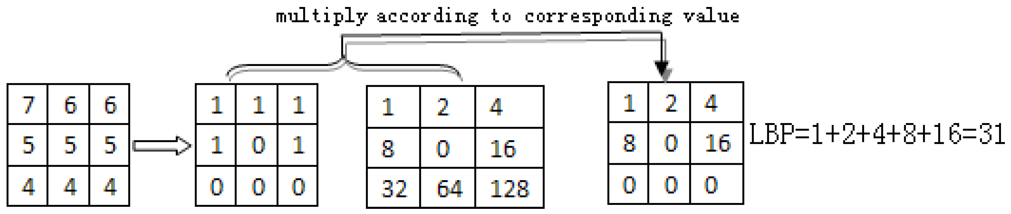
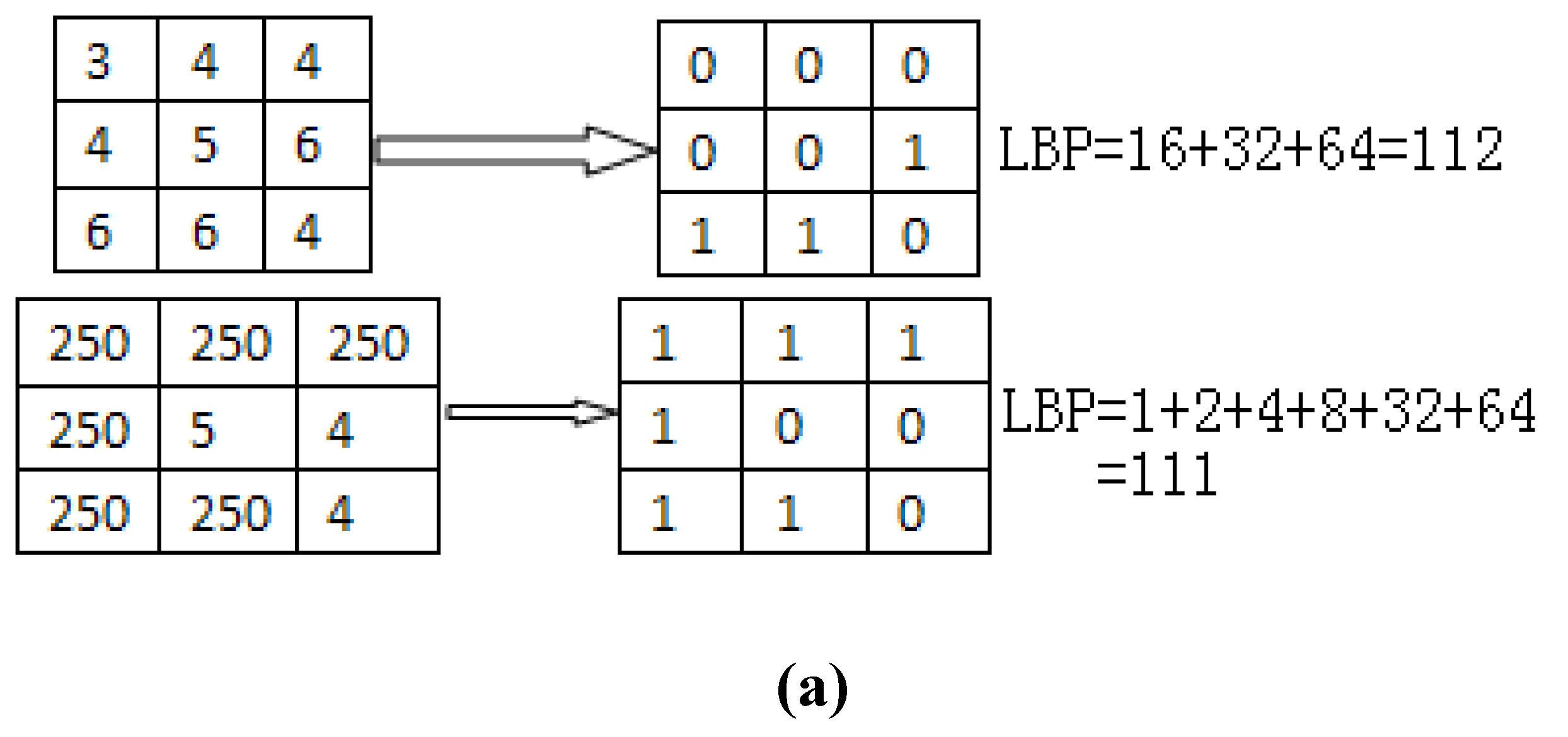
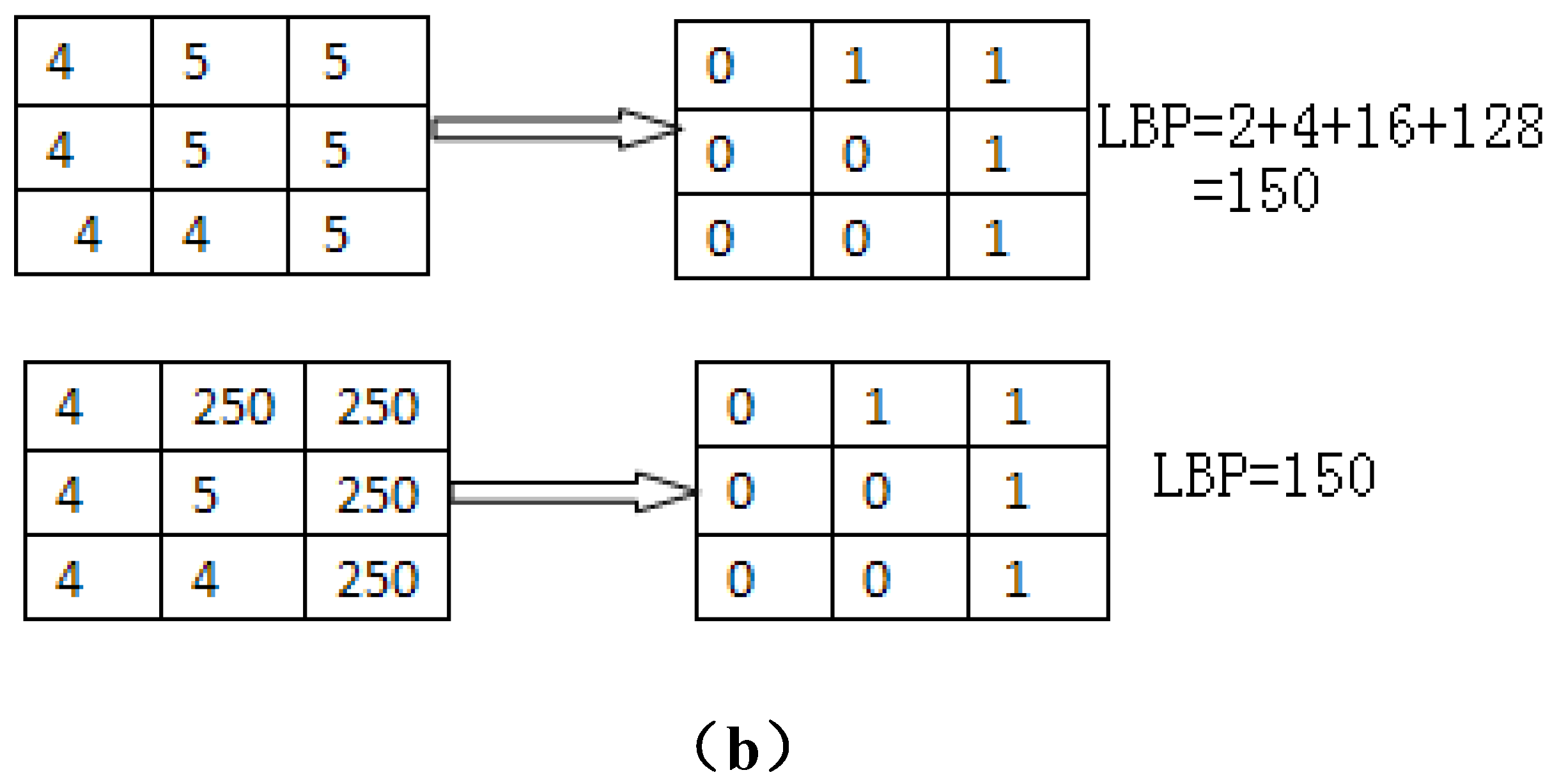
2. LBP Texture Operators

The LBP operator was first introduced by Ojala et al. [18]. It labels the pixels of an image by considering the difference between the grey values of the pixel x from the grey values of the circularly symmetric neighborhood and considers the results as a binary number. Given a pixel, LBP code can be expressed in the decimal form as equation (1), (2).

$$\mathrm{L}\mathrm{B}{\mathrm{P}}_{\mathrm{P},\mathrm{R}}={\displaystyle \sum _{p=0}^{p-1}sign(g_p-g_c)\cdot 2^p}$$

(1)

$$sign(x)=\{\begin{array}{l}1,x\ge 0\\ 0,x<0\end{array}$$

(2)

Where $g_c$ corresponds to the grey value of the center pixel of a local neighborhood and $g_p$ to the grey value of N equally spaced neighboring pixels. It produces $2^{\text{P}}$different output values, corresponding to the $2^{\text{P}}$ different binary patterns. The $2^{\text{P}}$ different binary patterns codify local primitives including different types of curved edges, spots, flat areas, etc. So each LBP code can be regarded as a micro-texture. The result over the 3 × 3 neighborhood as a binary number is described as follows (Figure 1).

Figure 1. The computational process of local binary pattern (LBP) code

Figure 1. The computational process of local binary pattern (LBP) code

We can see that the LBP code is robust against illumination changes and very fast to compute, and does not require many parameters to be set. However, LBP cannot describe the characteristics of textures efficiently and completely. In Figure 2, the first structure of (a) and (b) is possibly a flat area, and the second structure is possibly an edge or a spot. However, the value of LBP is uniform. So LBP ignores the contrastive information while the different contrast is an important feature of texture.

Figure 2. The incorrect instance of LBP texture

Figure 2. The incorrect instance of LBP texture

3. The PSO Algorithm

Particle swarm optimization is an evolutionary optimization technique created by inspiring behaviors such as fish schooling and bird flocking. The system is initialized with a population of random solutions and searches for optima by updating generations.

Suppose that the search space is D-dimensional. At the beginning of the PSO process, the position $Z_i=\left\{z_{i1},z_{i2,}\dots ,z_{id}\right\}$ and the velocity $V_i=\left\{v_{i1},v_{i2,}\dots ,v_{id}\right\}$ of each particle are randomly created. Every particle in the swarm is a part of the solution set. $y_i=\left\{y_{i1},y_{i2,}\dots ,y_{id}\right\}$ is the best position discovered by the ith individual. $\widehat{y}=\left\{{\widehat{y}}_1,{\widehat{y}}_2,\dots ,{\widehat{y}}_d\right\}$ stands for the global best position searched by the whole swarm. In each iteration, $Z_i$ and $V_i$ are updated using the following equation (3), (4).

$$v_{ij}\left(t+1\right)=\omega *v_{ij}\left(t\right)+c_1{r}_1\left(y_{ij}\left(t\right)-x_{ij}\left(t\right)\right)+c_2{r}_2\left({\widehat{y}}_j\left(t\right)-x_{ij}\left(t\right)\right)$$

(3)

$$z_{ij}\left(t+1\right)=z_{ij}\left(t\right)+v_{ij}\left(t+1\right)$$

(4)

Where $c_1$ and $c_2$ are the acceleration coefficients which determine the extent of stochastic weighting for the cognitive and the social components individually. $r_1$,$r_2$ are two random numbers generated by uniform distribution in the range [0,1] separately. The inertia weight $\omega$ is employed to control the impact of the previous history of velocities on the current velocity. The linear decreasing method is represented as equation (5).

$$\omega ={\omega }_{max}-\frac{{\omega }_{max}-{\omega }_{min}}{Ite{r}_{max}}\times iter$$

(5)

$Ite{r}_{max}$ is maximum iteration time. $iter$ is current iteration time. ${\omega }_{max}$ and ${\omega }_{min}$ are maximum and minimum inertia weight respectively (it is set for ${\omega }_{max}$= 0.9, ${\omega }_{min}$= 0.4). The inertia weight is decreased linearly with increasing iterations.

The solution quality is measured by the fitness function. The fitness value of each particle is calculated by the objective function. The values of $y_i$ and $\widehat{y}$ are then evaluated and replaced if a better particle best position or a better global best position is obtained. The smaller objective function is, the better fitness value is, given that objective function is expressed as equation (6). The fitness value is represented as equation (7) (to avoid zero in the denominators, $\text{σ}=0.001$).

$$J={\displaystyle \sum _{k=1}^C{\displaystyle \sum _{i=1}^N\Vert x_i-z_k\Vert }}$$

(6)

$$fitness=1/(J+\sigma )$$

(7)

The personal best position of each particle is defined as equation (8).

$$y_{ij}\left(t+1\right)=\{\begin{array}{c}{y}_{ij}\left(t\right),if fitness\left(z_{ij}\left(t+1\right)\right)\le fitness\left(y_{ij}\left(t\right)\right)\\ z_{ij}\left(t+1\right),if fitness\left(z_{ij}\left(t+1\right)\right)>fitness\left(y_{ij}\left(t\right)\right)\end{array}$$

(8)

The global best position is defined as equation (9).

$$\widehat{y}=\left\{{\widehat{y}}_1,{\widehat{y}}_2,\dots ,{\widehat{y}}_d\right\}|fitness\left(\widehat{y}\right)=max\left\{fitness\left(y_1\left(t\right)\right),fitness\left(y_2\left(t\right)\right),\dots ,fitness\left(y_s\left(t\right)\right)\right\}$$

(9)

Then we can use the standard procedure to find the optimum. The searching is a repeated process, and the stop criteria are that the maximum iteration number is reached or the minimum error condition is satisfied.

4. The Proposed Method

4.1. Feature Extraction

Given that a RGB color image is commonly represented as array $H\times W\times l$ where every pixel $f_l\left(i,j\right)$ is a vector of integer values between the interval of [0, 255] (for color image $l$ = 3). LBP code of $f_l\left(i,j\right)$ is represented as $LBP\left(i,j\right)$. We combine LBP code of color components as equation (10).

$$LBP(i,j)={\displaystyle \sum _{p=0}^{p-1}sign({\displaystyle \sum _{i=1}^l(g_{lp}-g_{lc}})})\cdot 2^p$$

(10)

To consider contrastive information, we use the mean of the min-max difference to discriminate the incorrect instance of LBP of Figure 2. S represents the mean of the min-max difference in equation (11). In the flat area, the mean of the min-max difference is nearly 0. For edges or spots, the mean of the min-max difference is larger. Therefore, it can reflect the change of contrastive information. In equation (11), $\sqrt{3}$ limits the values in the interval of [0, 255].

$$S=\frac{1}{\sqrt{3}p}·{\displaystyle \sum }_{p=0}^{p-1}{\Vert g_{lp}-g_{lc}\Vert }_{\mathrm{∎}}$$

(11)

${\Vert {\text{g}}_{\text{lp}}-{\text{g}}_{\text{lc}}\Vert }_{\mathrm{∎}}$represents Euclidean distance.

We use LBP, the mean of the min-max difference, color components as segmental features, and merge above features as feature vector $\left({\text{f}}_1\left(\text{i},\text{j}\right),{\text{f}}_2\left(\text{i},\text{j}\right),{\text{f}}_3\left(\text{i},\text{j}\right),\text{LBP},\text{S}\right)$.

4.2. Improving FCM Algorithm

PSO takes real numbers as particles. It is theoretically simple and can be implemented in a few lines of code. But PSO easily gets stuck in local optima. An effective way to overcome premature convergence of basic PSO is to maintain the population diversity for exploring the new search domain during the evolution process. We propose an improved optimization algorithm by adding mutation operator of genetic algorithm (GA) to PSO. The hybrid algorithm combines the standard velocity and position update rules of PSO with mutation operator from GA and makes the search jump out of local optima.

To improve the FCM algorithm, we utilize the texture information for each pixel to define a spatial constraint term, and then introduce this spatial constraint term into the objective function of FCM. The modified objective function can be expressed as equation (12)

$$J=\alpha {\displaystyle \sum _{k=1}^K{\displaystyle \sum _{i=1}^H{\displaystyle \sum _{j=1}^W{{\mu }_{kij}}^m\Vert f_l(i,j)-z_{kl}\Vert }}}+\beta {\displaystyle \sum _{k=1}^K{\displaystyle \sum _{i=1}^H{\displaystyle \sum _{j=1}^W{{\mu }_{kij}}^m\Vert LBP-z_{kl}\Vert }}}+\gamma {\displaystyle \sum _{k=1}^K{\displaystyle \sum _{i=1}^H{\displaystyle \sum _{j=1}^W{{\mu }_{kij}}^m\Vert S-z_{kl}\Vert }}}$$

(12)

To add spatial information, we use the above feature vector to complete clustering. ${\mu }_{kij}$ is a membership matrix where each value represents the membership grade of $f_l$ (i,j) which belongs to the kth class in equation (13). $z_{xk}$ is the clustering centre. $z_{lk}$ represents represent the clustering center of the color component which is the color feature. $z_{4k}$ represents the clustering centre of LBP code. $z_{5k}$ represents the clustering center of the mean of difference in equation (14). LBP code and $z_{5k}$represent the texture feature of the area. m is a weighting exponent that determines the amount of fuzziness of the resulting classification (in this paper, m = 2). $\alpha , \beta , \gamma$ are weights that are manually determined in a trial-and-error fashion (in this paper, $\alpha =0.1, \beta =0.1, \gamma =0.8$). Through merging feature vector, the distance between pixels is more accurate.

$${\mu }_{kij}=\frac{1}{{{\displaystyle \sum _{k_1=1}^C(\frac{\alpha (LBP(i,j)-z_4(k))+\beta (S(i,j)-z_5(k))+\gamma {\Vert f_l(i,j)-z_l(k)\Vert }_{•}}{\alpha (LBP(i,j)-z_4(k_1))+\beta (S(i,j)-z_5(k_1))+\gamma {\Vert f_l(i,j)-z_l(k_1)\Vert }_{•}})}}^{2/(m-1)}}$$

(13)

$$\{\begin{array}{l}{z}_{lk}=\frac{{\displaystyle \sum _{i=1}^{H^{\prime }}{\displaystyle \sum _{j=1}^{W\prime }{({\mu }_{kij})}^m}}(f_l(i,j))}{{\displaystyle \sum _{i=1}^{H^{\prime }}{\displaystyle \sum _{j=1}^{W\prime }{({\mu }_{kij})}^m}}}\\ z_{lk}=\frac{{\displaystyle \sum _{i=1}^{H^{\prime }}{\displaystyle \sum _{j=1}^{W\prime }{({\mu }_{kij})}^m}}(LBP(i,j))}{{\displaystyle \sum _{i=1}^{H^{\prime }}{\displaystyle \sum _{j=1}^{W\prime }{({\mu }_{kij})}^m}}}\\ z_{lk}=\frac{{\displaystyle \sum _{i=1}^{H^{\prime }}{\displaystyle \sum _{j=1}^{W\prime }{({\mu }_{kij})}^m}}(S(i,j))}{{\displaystyle \sum _{i=1}^{H^{\prime }}{\displaystyle \sum _{j=1}^{W\prime }{({\mu }_{kij})}^m}}}\end{array}$$

(14)

The proposed algorithm is described as follows.

Step 1: Set the iteration number $\text{ iter}$ to zero, $Ite{r}_{max}=5$. An initial swarm of particles is generated in the search space. The population size is set to N (in this paper, $N=20$). The position $z_{ij}$ and the velocity $v_{ij}$ of each particle are randomly created. Given ${\omega }_{max}=0.9$,${\omega }_{min}=0.4,$ mutation probability ${\text{p}}_{\text{m}}=0.05$.

Step 2: Computer $\text{ω}$ by using equation (5) and evaluate the fitness of each particle by using equation (7).

Step 3: Compare the personal best of each particle to its current fitness and set the personal best of each particle to the better performance.

Step 4: Set the global best to the position of the particle with the best fitness within the swarm.

Step 5: Change the velocity vector for each particle according to equation (3).

Step 6: Move each particle to its new position, according to equation (4).

Step 7: Randomly choose $p$, when $p>p_m$, the position of each particle will apply mutation operator.

Step 8: Let $iter=iter+1$. Go to step 2. And repeat until meets the stop criteria $iter>Ite{r}_{max}$.

Step 9: Make the position $z_{ij}$ as initial cluster centers, initializes membership matrix u_kij for random value between 0, 1.

Step 10: Use the membership matrix u_ij calculated in equation (13).

Step 11: According to equation (14), calculate cluster centers. If the relative change between $\stackrel{\rightharpoonup }{v_{old}}$ and $\stackrel{\rightharpoonup }{v_{new}}$ are less than a certain threshold (($\stackrel{\rightharpoonup }{\Vert v_{new}}-\stackrel{\rightharpoonup }{v_{old}}\Vert <\epsilon$) (in this paper, $\text{ ε}=10$)), then the algorithm stops. Otherwise, return to Step 10.

5. Experiments

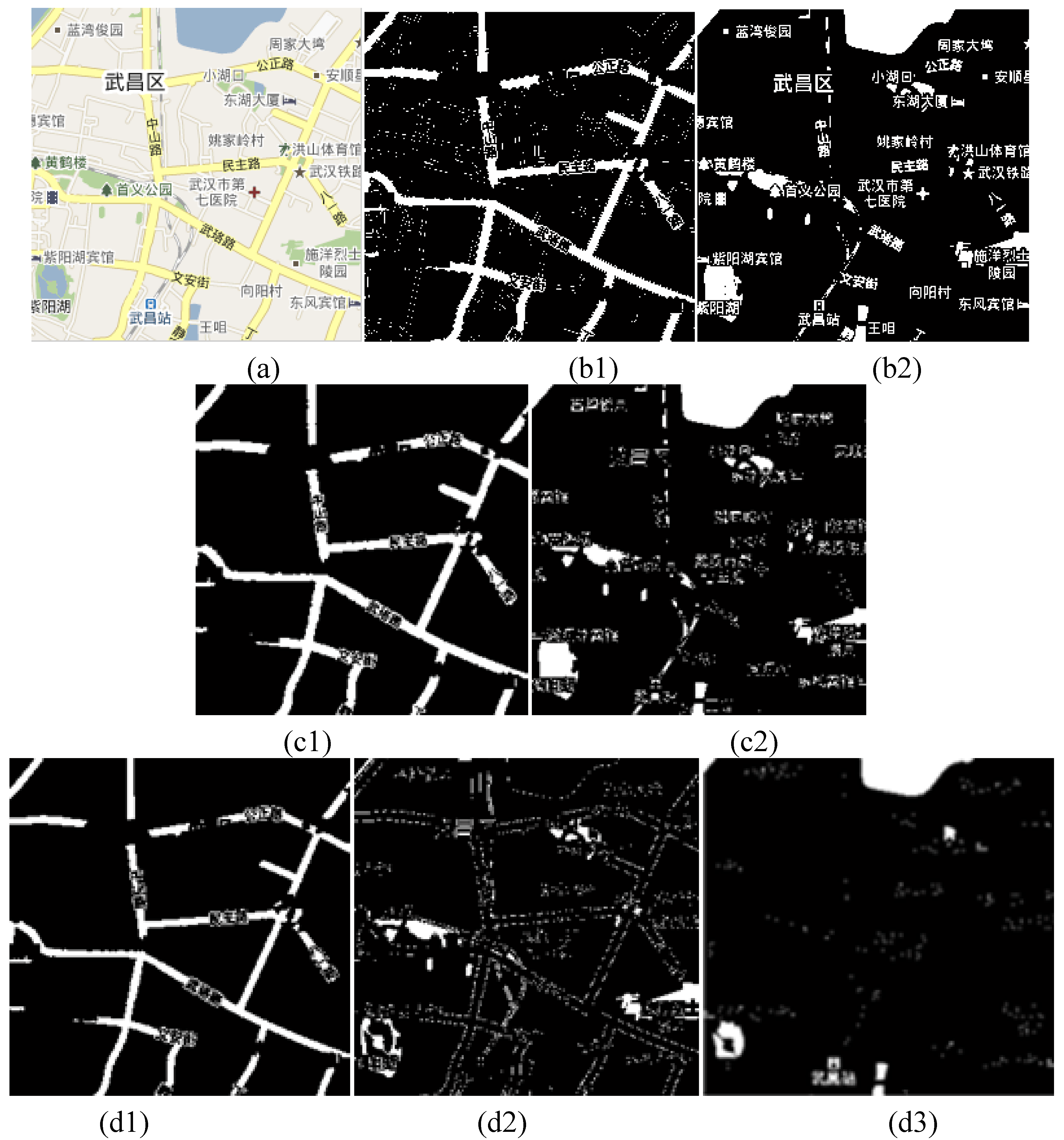
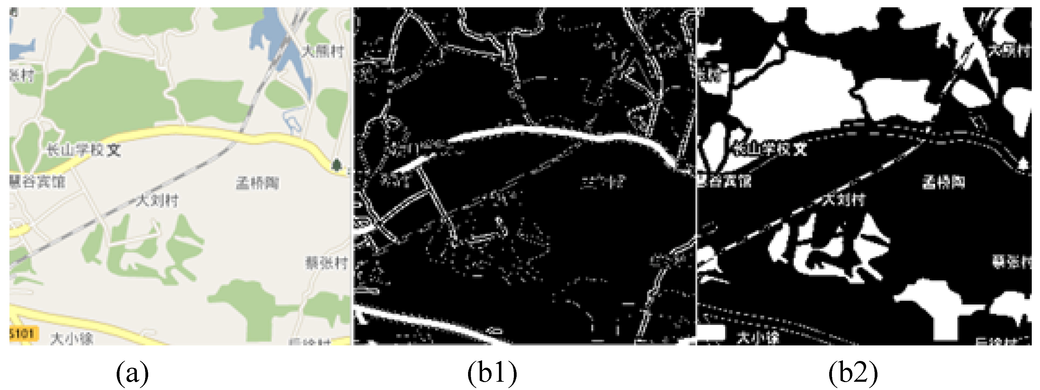
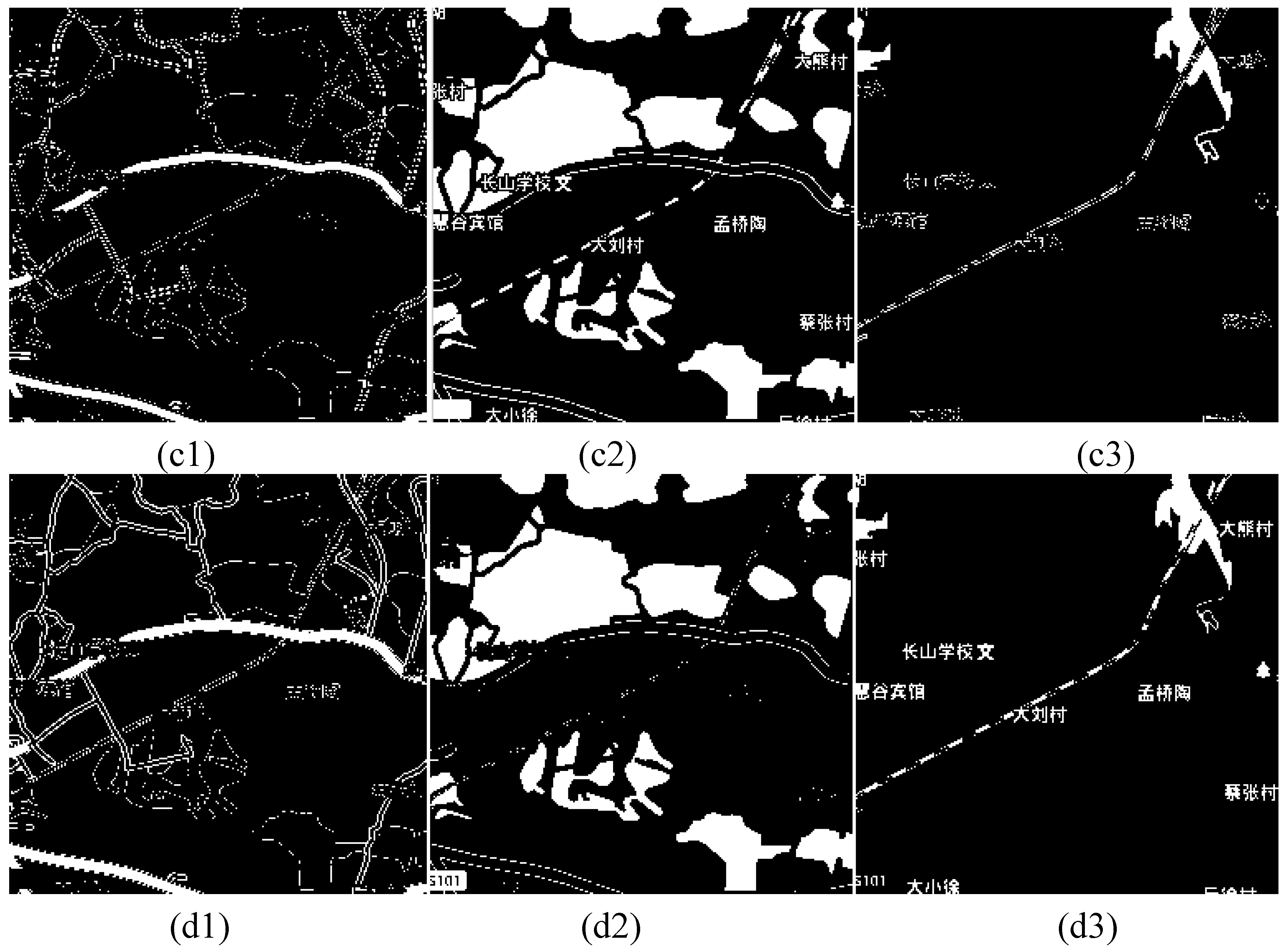
5.1. Multi-Feature Optimization Clustering Segmentation

In the experiments, we test with several 256 × 256 color images which are obtained from WebGIS (for example, Google Map/Earth) to assess the performance of the proposed algorithm with Matlab7.0 running on a desktop PC with 2.0GHz CPU and 1.0G RAM. The results of kernel-based FCM with prototypes in feature space (KFCM_F), FCM with spatial constraints (FCM_S) and the proposed method are compared.

Figure 3 (a) is “map1” original image. In KFCM_F and FCM_S, the initial class is set to 7. Figure 3 (b), (c), (d) shows the results of “map1” image segmentation. KFCM_F and FCM_S only divide the image into 3 classes. They use a separate color feature and cannot segment accurately. The proposed method divides the image into 7 classes. Figure 3 (b1), (b2) are the “road” and “lake” of KFCM_F. Figure 3 (c1), (c2) are the “road” and “lake” of FCM_S. We can see that in KFCM_F and FCM_S the “lake” and “terrain” are considered to be the same and cannot be segmented exactly. Figure 3 (d1), (d2), (d3) are the “road”, “terrain” and “lake” of the proposed method. It can be seen that the proposed method has a better performance to segment accurately the “road”, “terrain” and “lake”.

Figure 4 (a) is “map2” original image. Figure 4 (b1), (b2) are the “road” and “lake” of KFCM_F. Figure 4 (c1), (c2), (c3) are the result of FCM_S. Figure 4 (d1), (d2), (d3) are the “road”, “terrain” and “lake” of the proposed method. Each method divides the image into five classes. Since KFCM_F and FCM_S can easily get into local optimization, we can see that from Figure (b2), the “lake” and “terrain” of KFCM_F are segmented into the same class. The “road” segmented from KFCM_F and FCM_S have less irrelevant information, but other shapes are mixed and cannot be segmented accurately. The proposed method can avoid getting into local optimization to get an overall better segmentation result.

Figure 3. The segmentation result of “map1” image: (a) “map1” original image; (b1) “road” of KFCM_F; (b2) “lake” of KFCM_F; (c1) “road” of FCM_S; (c2) “lake” of FCM_S; (d1) “road” of the proposed method; (d2) “terrain” of the proposed method; (d3) “lake” of the proposed method.

Figure 3. The segmentation result of “map1” image: (a) “map1” original image; (b1) “road” of KFCM_F; (b2) “lake” of KFCM_F; (c1) “road” of FCM_S; (c2) “lake” of FCM_S; (d1) “road” of the proposed method; (d2) “terrain” of the proposed method; (d3) “lake” of the proposed method.

Figure 4. The segmentation result of “map2” image: (a) “map2” original image; (b1) “road” of KFCM_F; (b2) “lake” of KFCM_F; (c1) “road” of FCM_S; (c2) “terrain” of FCM_S; (c3) “lake” of FCM_S; (d1) “road” of the proposed method; (d2) “terrain” of the proposed method; (d3) “lake” of the proposed method.

Figure 4. The segmentation result of “map2” image: (a) “map2” original image; (b1) “road” of KFCM_F; (b2) “lake” of KFCM_F; (c1) “road” of FCM_S; (c2) “terrain” of FCM_S; (c3) “lake” of FCM_S; (d1) “road” of the proposed method; (d2) “terrain” of the proposed method; (d3) “lake” of the proposed method.

5.2. Post-Processing

To get more accurate results, we can implement post-processing by using the morphological method. Given $f(i,j)$ is the segmental result of the proposed method. We use two times fusion operator, then two times dilation operator. E represents fusion operator. D represents dilation operator.

$$F(i,j)=E^2(f)D^2(f)$$

(15)

Figure 5. The post-processing result of Figure 3(d) and Figure 4(d): (a1) the “road” of Figure 3(d1); (a2) the “lake” of Figure 3(d3); (a3) the “terrain” of Figure 3(d2); (b1) the “road” of Figure 4(d1); (b2) the “lake” of Figure 4(d3); (b3) the “terrain” of Figure 4(d2).

Figure 5. The post-processing result of Figure 3(d) and Figure 4(d): (a1) the “road” of Figure 3(d1); (a2) the “lake” of Figure 3(d3); (a3) the “terrain” of Figure 3(d2); (b1) the “road” of Figure 4(d1); (b2) the “lake” of Figure 4(d3); (b3) the “terrain” of Figure 4(d2).

Figure 5 shows the post-processing results of Figure 3 (d) and Figure 4 (d). Figure 5 (a1) is the post-processing “road” of Figure 3 (d1). Figure 5 (a2) is the post-processing “lake” of Figure 3 (d3). Figure 5 (a3) is the post-processing “terrain” of Figure 3 (d2). Figure (b1) is the post-processing “road” of Figure 4 (d1). Figure 5 (b2) is the post-processing “lake” of Figure 4 (d3). Figure 5 (b3) is the post-processing “terrain” of Figure 4 (d2).

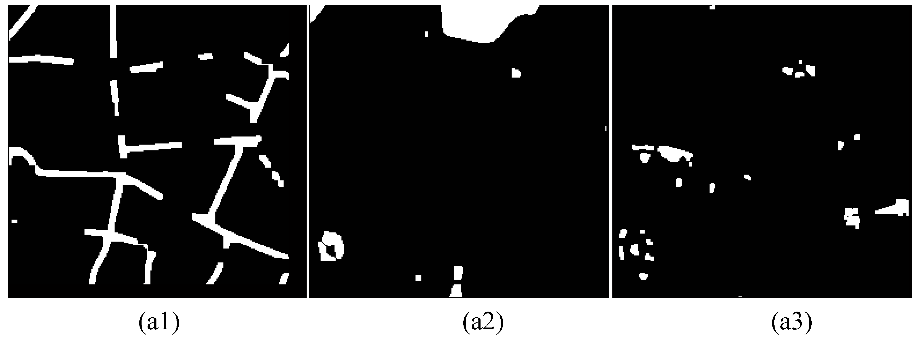
5.3. Ratio of Misclassification

To compare the proposed method with existing methods, we use the ratio of misclassification to evaluate the different algorithms. We define the ratio of misclassification as equation (16).

$$Error=\frac{\sum \left|s-v\right|}{\sum s}\times 100\%$$

(16)

s is the binary image of manual segmentation. v is the binary image of actual segmentation by algorithms. The absolute difference between the binary images s and v is the number of misclassification. ${\sum }^{\text{}}\text{s}$ is the total number of pixels for the manual segmental image. Figure 6 is the manual segmentation result.

Figure 6. The manual segmentation result of Figure 3(a): (a1) the “road” of manual segmentation (a2) the “lake” of manual segmentation (a3) the “terrain” of manual segmentation.

Figure 6. The manual segmentation result of Figure 3(a): (a1) the “road” of manual segmentation (a2) the “lake” of manual segmentation (a3) the “terrain” of manual segmentation.

According to equation (16), the ratios of misclassification are shown in Table 1. The ratio of misclassification of “road” is lowest in KFCM_F and FCM_S, however, still higher than the proposed method which is 10.24% and can basically segment “road” accurately. For “terrain” segmentation, the result of KFCM_F is the worst, and the ratio of misclassification is 30.05%. The result of FCM_S is better with adding spatial information. The proposed method is the best in “terrain” segmentation, and the accuracy has achieved 95%. For “lake” segmentation, FCM_S and KFCM_F have much more errors. The proposed method can segment “lake” very accurately.

Table 1. The ratio of misclassification of difference methods.

	Algorithm	KFCM_F	FCM_S	The proposed
“map1” image	The ratios of misclassification of “lake”	35.70%	31.00%	1.1%
	The ratios of misclassification of “terrain”	32.05%	19.56%	5.05%
	The ratios of misclassification of “road”	20.33%	15.81%	10.24%

Table 1. The ratio of misclassification of difference methods.

	Algorithm	KFCM_F	FCM_S	The proposed
“map1” image	The ratios of misclassification of “lake”	35.70%	31.00%	1.1%
	The ratios of misclassification of “terrain”	32.05%	19.56%	5.05%
	The ratios of misclassification of “road”	20.33%	15.81%	10.24%

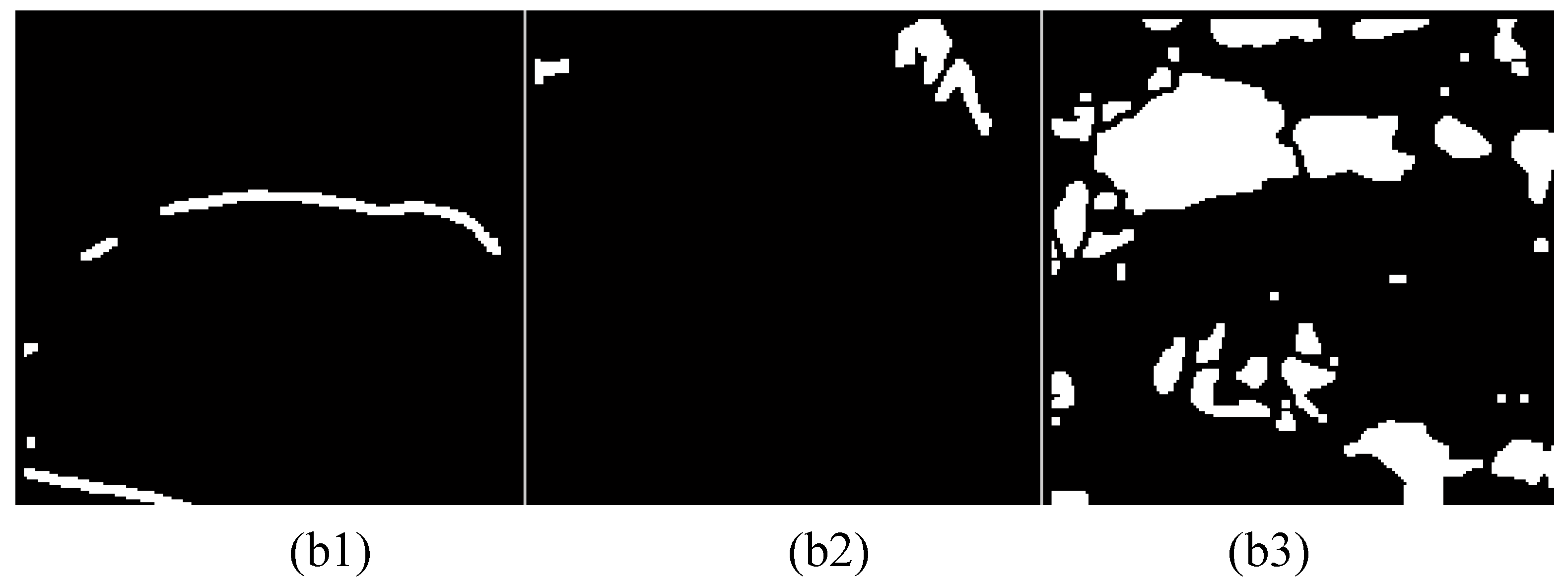
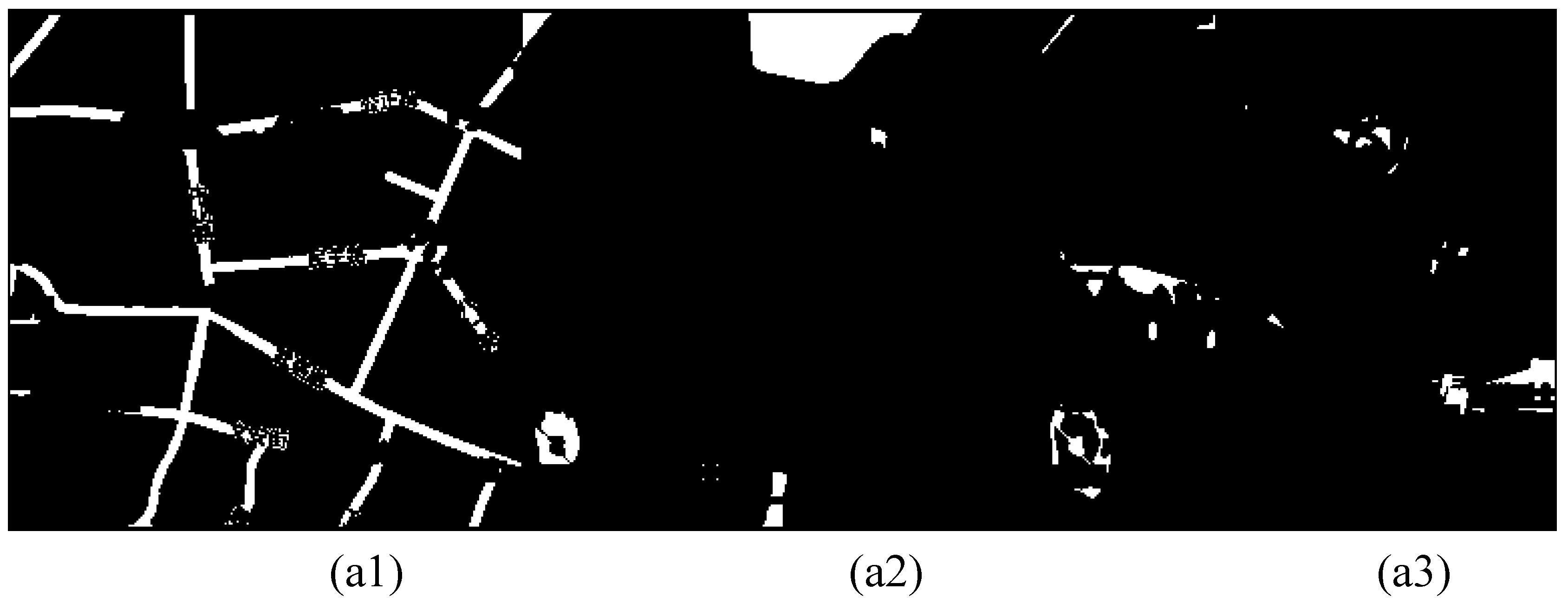
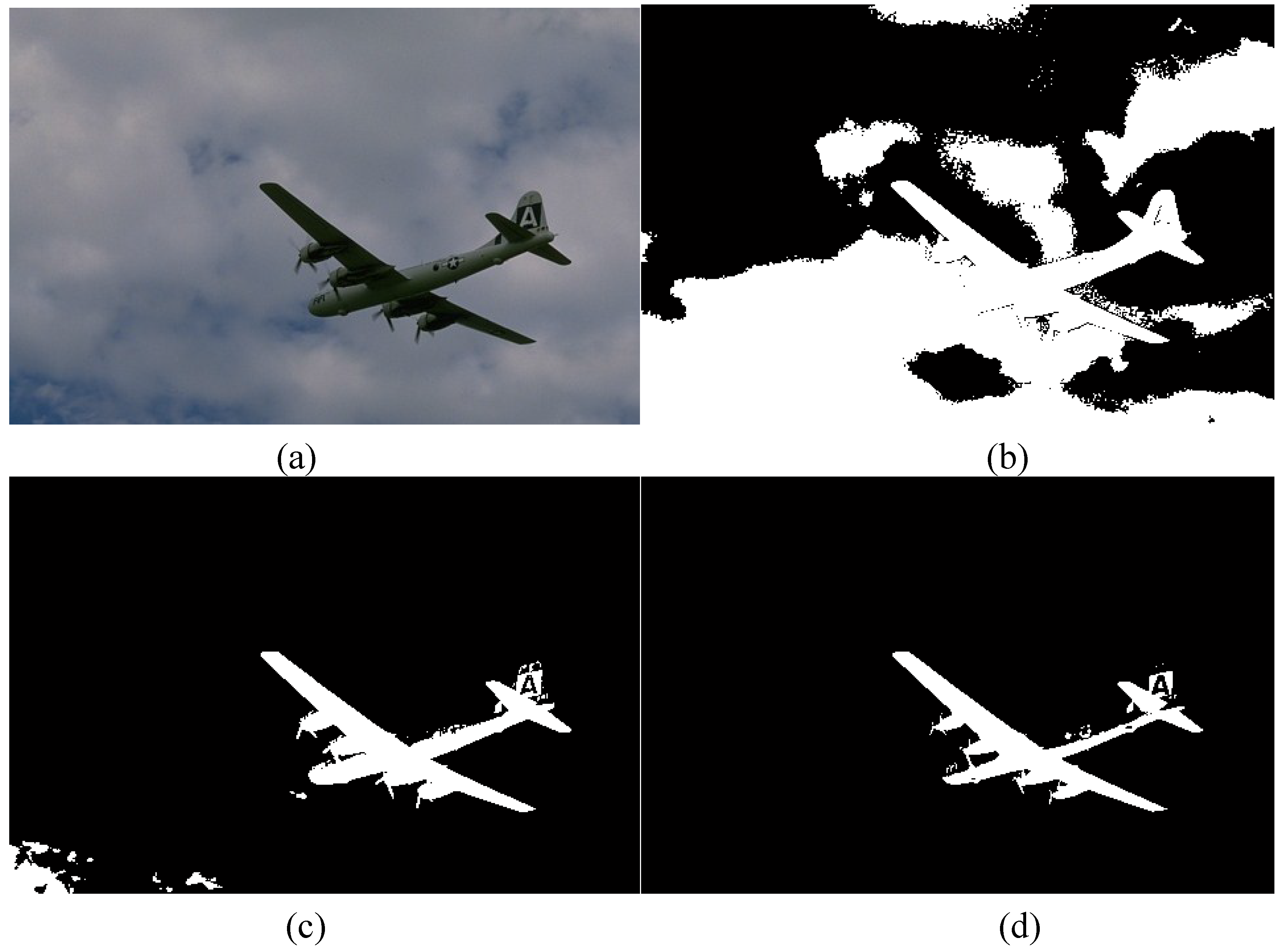
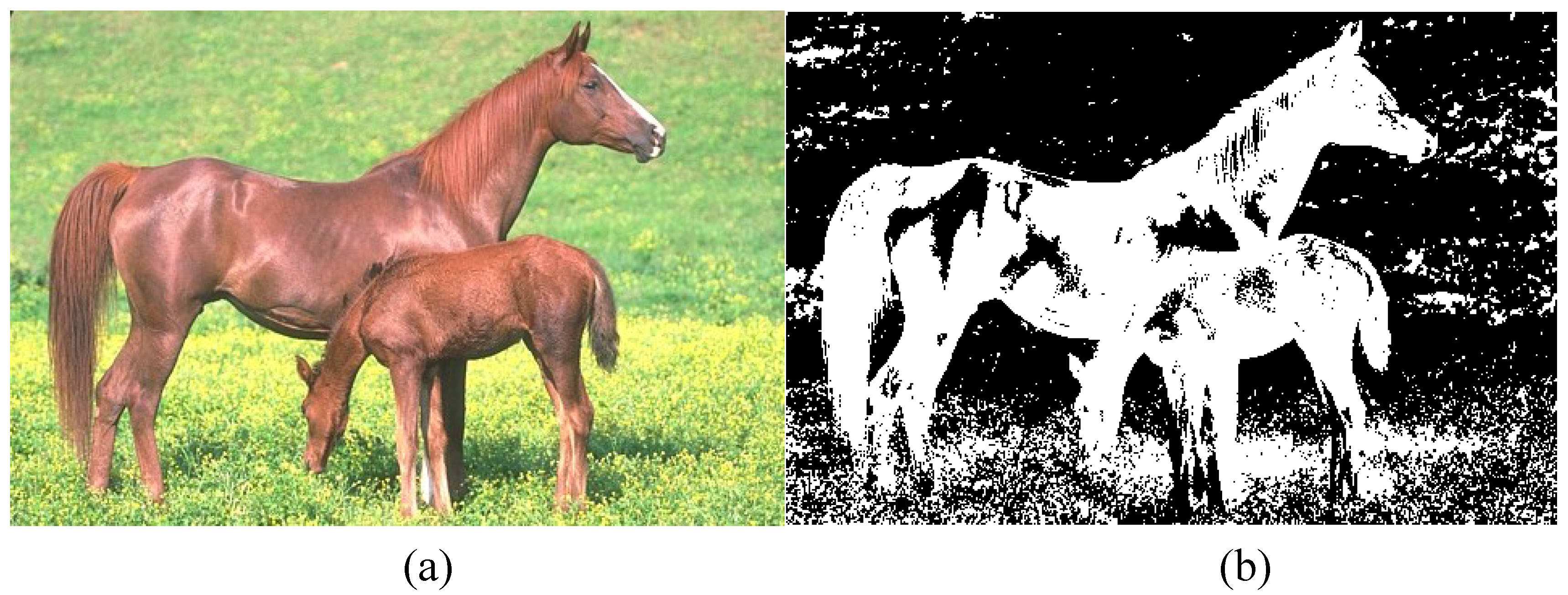
5.4 Extended Experiments for Target Extraction

In addition, we test target extraction with real images in database [19] to assess the performance of the proposed algorithm by Matlab7.0. Figure 7(a) is the original “horse” image. Figure 7(b) is its segmentation result of KFCM_F. Figure 7(c) is its segmentation result of FCM_S. Figure 7(d) is its segmentation result of the proposed method. Figure 8(a) is the original “plane” image. Figure 8(b) is its segmentation result of KFCM_F. Figure 8(c) is its segmentation result of FCM_S. Figure 8(d) is its segmentation result of the proposed method. Comparing the proposed segmentation results with the existing methods, it can be seen that KFCM_F cannot segment the objects accurately as a lot of unrelated pixels are segmented into the object areas, while FCM_S has a certain randomness. The segmentation results of the proposed method are most accurate compared to KFCM_F and FCM_S.

Figure 7. The segmentation result of “horse” image: (a) “horse” original image; (b) the result of KFCM_F; (c) the result of FCM_S; (d) the result of the proposed method.

Figure 7. The segmentation result of “horse” image: (a) “horse” original image; (b) the result of KFCM_F; (c) the result of FCM_S; (d) the result of the proposed method.

Figure 8. The segmentation result of “plane” image: (a) “plane” original image; (b) the result of KFCM_F; (c) the result of FCM_S; (d) the result of the proposed method.

Figure 8. The segmentation result of “plane” image: (a) “plane” original image; (b) the result of KFCM_F; (c) the result of FCM_S; (d) the result of the proposed method.

6. Conclusions

In this paper, we propose a multi-feature optimization clustering algorithm for color image segmentation. We combine pixel and texture features as a feature vector to effectively improve segmentation performance. It utilizes PSO with mutation operator of GA to evaluate the initial clustering center, and ensures that the search converges faster and makes the search jump out of local optima. Experimental results show that the proposed algorithm can achieve better performance than other classic clustering algorithms in terms of segmentation accuracy.

References

1. Graves, D.; Pedrycz, W. Kernel-based fuzzy clustering and fuzzy clustering: A comparative experimental study. Fuzzy Sets Syst. 2010, 161, 522–543. [Google Scholar] [CrossRef]
2. Kannan, S.R.; Ramathilagam, S.; Devi, R.; Sathy, A. Robust kernel FCM in segmentation of breast medical images. Expert Syst. Appl. 2011, 38, 4382–4389. [Google Scholar] [CrossRef]
3. Mújica-Vargas, D.; Gallegos-Funes, F.J.; Rosales-Silva, A.J. A fuzzy clustering algorithm with spatial robust estimation constraint for noisy color image segmentation. Pattern Recognit. Lett. 2013, 34, 400–413. [Google Scholar] [CrossRef]
4. Zhao, F.; Jiao, L.C.; Liu, H.Q.; Gao, X.B. A novel fuzzy clustering algorithm with non-local adaptive spatial constraint for image segmentation. Signal Process. 2011, 91, 988–999. [Google Scholar] [CrossRef]
5. Qiu, C.; Xiao, J.; Yu, L.; Han, L.; Iqbal, M.N. A modified interval type-2 fuzzy C-means algorithm with application in MR image segmentation. Pattern Recognit. Lett. 2013, 34, 1329–1338. [Google Scholar] [CrossRef]
6. Costa, Y.M.G.; Oliveira, L.S.; Koerich, A.L.; Gouyon, F.; Martins, J.G. Music genre classification using LBP textural features. Signal Process. 2012, 92, 2723–2737. [Google Scholar] [CrossRef]
7. Shan, C.; Gong, S.; McOwan, P.W. Facial expression recognition based on Local Binary Patterns:A comprehensive study. Image Vis. Comput. 2009, 27, 803–816. [Google Scholar] [CrossRef]
8. Moore, S.; Bowden, R. Local binary patterns for multi-view facial expression recognition. Comput. Vis. Image Underst. 2011, 115, 541–558. [Google Scholar] [CrossRef]
9. Luo, Y.; Wu, C.; Zhang, Y. Facial expression recognition based on fusion feature of PCA and LBP with SVM. Int. J. Light Electron Optics. 2013, 124, 2767–2770. [Google Scholar] [CrossRef]
10. Liu, Y.; Chen, M.; Ishikawa, H.; Wollstein, G.; Schuman, J.S. Automated macular pathology diagnosis in retinal OCT images using multi-scale spatial pyramid and local binary patterns in texture and shape encoding. Med. Image Anal. 2011, 15, 748–759. [Google Scholar] [CrossRef] [PubMed]
11. Heikkila, M.; Ainen, M.; Schmid, C. Description of interest regions with local binary patterns. Pattern Recognit. 2009, 42, 425–436. [Google Scholar] [CrossRef]
12. Nanni, L.; Lumini, A. Local binary patterns for a hybrid fingerprint matcher. Pattern Recognit. 2008, 41, 3461–3466. [Google Scholar] [CrossRef]
13. Kennedy, J.; Eberhart, R. Particle swarm optimization. In Proceedings of the 1995 IEEE International Conference on Neural Networks, Perth, WA, USA, 1995; pp. 1942–1948.
14. Jie, J.; Zeng, J.; Han, C.; Wang, Q. Knowledge-based cooperative particle swarm optimization. Appl. Math. Comput. 2008, 205, 861–873. [Google Scholar] [CrossRef]
15. Tsai, C.; Kao, I. Particle swarm optimization with selective particle regeneration for data clustering. Expert Syst. Appl. 2011, 38, 6565–6576. [Google Scholar] [CrossRef]
16. Bedi, P.; Bansal, R.; Sehgal, P. Using PSO in a spatial domain based image hiding scheme with distortion tolerance. Comput. Elect. Engin. 2013, 39, 640–654. [Google Scholar] [CrossRef]
17. Vellasques, E.; Sabourin, R.; Granger, E. Fast intelligent watermarking of heterogeneous image streams through mixture modeling of PSO populations. Appl. Soft Comput. 2013, 13, 3130–3148. [Google Scholar] [CrossRef]
18. Ojala, T.; Pietikainen, M.; Harwood, D. A comparative study of texture measure with classification based on feature distribution. Pattern Recognit. 1996, 29, 51–59. [Google Scholar] [CrossRef]
19. The Berkeley Segmentation Dataset and Benchmark. Available online: http://www.eecs.berkeley.edu/Research/Projects/CS/vision/bsds/ (accessed on 4 May 2015).