1. Introduction
The numerical solution of nonlinear equations and systems is widely used in different branches of Science and Technology, as in the analysis of diffusion phenomena (see, for example, [
1,
2]), the study of dynamical models of chemical reactors [
3], the numerical computing of the dominant eigenvalue of the neutron transport criticality problem (see [
4]), the study of radioactive transfer [
5], or in the orbit determination of artificial satellites (see [
6]), among others.
Burgers’ equation arises in the theory of shock waves, in turbulence problems and in continuous stochastic processes. It has a large variety of applications: modeling of water in unsaturated oil, gas dynamics, heat conduction, elasticity, statics of flow problems, mixing and turbulent diffusion, cosmology, seismology,
etc. (see [
7] and the references therein).
We consider the one-dimensional Burgers’ equation
with initial condition
,
, and boundary conditions
,
,
; where
is the Reynolds number of the viscous fluid flow problem and
,
and
are given functions. Usually ε instead of
is used, for simplicity. Numerical difficulties have been experienced in getting the solution of Burgers’ equation for big values of ε.
This problem shows a roughly similar structure to that of Navier-Stokes equations due to the form of the nonlinear convection term and the occurrence of the viscosity term. So, this can be considered as a simplified form of the Navier-Stokes equation. In recent years, many researchers have used different numerical methods specially based on finite difference, finite element boundary techniques and direct variational methods to solve this problem (see, for example, [
7,
8,
9] and the references therein). It has been shown by Hopf and Cole that Burgers’ equation can be solved exactly for an arbitrary initial function
. The transformation
relates
and
, and if ϕ is a solution of the linear diffusion equation
then
u is a solution of the quasilinear Burgers’ Equation (1). This transformation let us obtain the exact values of
because Equation (3) has a Fourier series solution, however its computational cost is very high and we only use it for comparing the precision of our results (as we will see in the Numerical Section, the integrals of the Fourier coefficients must be calculated). As we can see in [
7], some researchers have taken advantage of this transformation and have applied the Crank-Nicolson scheme to the linear Equation (3) in order to obtain the values of
and after it the values of
. Other authors have used the implicit scheme, where
is approximated by backward differences, however, due to its truncation error has order one, the precision of the results decreases.
In this paper, we apply a particular difference scheme called Crank-Nicolson type method, obtained by applying divided differences directly on the nonlinear Equation (1), needing to solve a nonlinear system of equations for obtaining the solution in each value of
t. These nonlinear systems are solved by using fixed point iterative methods. In particular, we are going to use the classical Newton’s method of order two,
Traub’s method of order three (see [
10])
and the method denoted by M5 (see [
11]) of fifth order of convergence, whose expression is reminded in the following
In these iterative expressions,
denotes the vectorial real function that describes the nonlinear system and
is the associated Jacobian matrix.
The stability of the method is numerically analyzed and found to be unconditionally stable. The presented method has the accuracy of second order in space and time. We test our method by using several values of ε and different initial conditions in order to analyze its stability and consistence, and for doing this it is compared with other known methods and with the exact solution. From these numerical results several interesting conclusions are obtained.
2. Development of the Procedure
The easiest way to discretize a partial differential equation problem (like we have on Equation (1)) consist on reducing the continuous domain into an equispaced finite number of points
located on the nodes of a uniform rectangular mesh. The partial derivatives of
u can be estimated now by the following difference quotients
which are called forward differences and have a truncation error of order 1. The partial derivatives of
u can also be obtained by
which are backward differences and have also a truncation error of order 1. Finally the partial derivatives of
u can also be obtained by the following
which are called central differences and have a truncation error of order 2. In these expressions,
denotes the approximated value of the unknown
u function on
,
and
are respectively the space and time step on the mesh and
n and
m are respectively the space and time amount of subintervals to be considered. Then, we consider
and
, where
and
.
Let us apply Crank-Nicolson difference scheme, which consists of discretizing Equation (1) in two consecutive time instants of
j and average them. In the first instant
we approximate
by the forward difference described on Equation (7) and in the second instant
we do it by the backward one. At both instants we approximate
and
by using the central differences (described by Equations (9) and (10) respectively). By means of this procedure we get, for the first instant,
and for the second one,
After averaging both expressions, it results
where
,
,
and the range of indices is
and
. This expression (which has a truncation error of order 2) results on a
m nonlinear systems of
unknowns and
equations. Each one of these systems comes after considering that we already know the value of
and
,
(from the boundary conditions) and
,
from the initial condition. Let us notice that the values corresponding to the
j subindex have been calculated on the previous systems and the only unknowns will be those with the
subindex.
3. Numerical Results
We are comparing our results with the exact solution, which can be obtained by the Hopf-Cole transformation mentioned on Equations (2) and (3). For doing this, we first calculate
and after it, by Equation (2), we obtain
where
Our goal is to obtain at least five exact decimals from the exact solution in order to prove the precision of our results, and for that we have seen that it is enough with two summands of the Fourier series, thereby only
,
and
will have to be calculated.
In the following examples we consider that the boundary conditions are zero, so we have that
and
, what means that
and
,
. We can compare our results with the exact solution in this case, however our method has been found numerically to be unconditionally stable whatever the boundary conditions are. We use the R2013a version of Matlab with double precision for obtaining both approximated and exact solutions. The stopping criterion used is
Example 1. The initial and boundary conditions of Burgers’ equation for this example are
and
where
and
.
In the following tables we show, for different values of n, m and ε, the average number of iterations by using Newton’, Traub’s and M5 methods. We also show the greatest error, GE, that we obtain for every value of and , where and . The initial approximation of each nonlinear system to be solved is the solution of the previous one (and for the first system the initial approximation is the exact value of the initial condition). After that, we obtain the matrix of errors as the absolute difference between the approximated solution and the exact solution on each node, finally we call the greatest error as the greatest element from that matrix. While other authors prefer to only compare and give the value of the error in some points of the mesh we have preferred a more rigorous criterium, it consists on comparing all the error values from the matrix of errors and giving the value of GE, in this way we get a better idea about how bad is the worst possible situation and we know for sure that the error of the rest of the points will always be below this GE, the other way we can not know if there is some point that has a greater one.
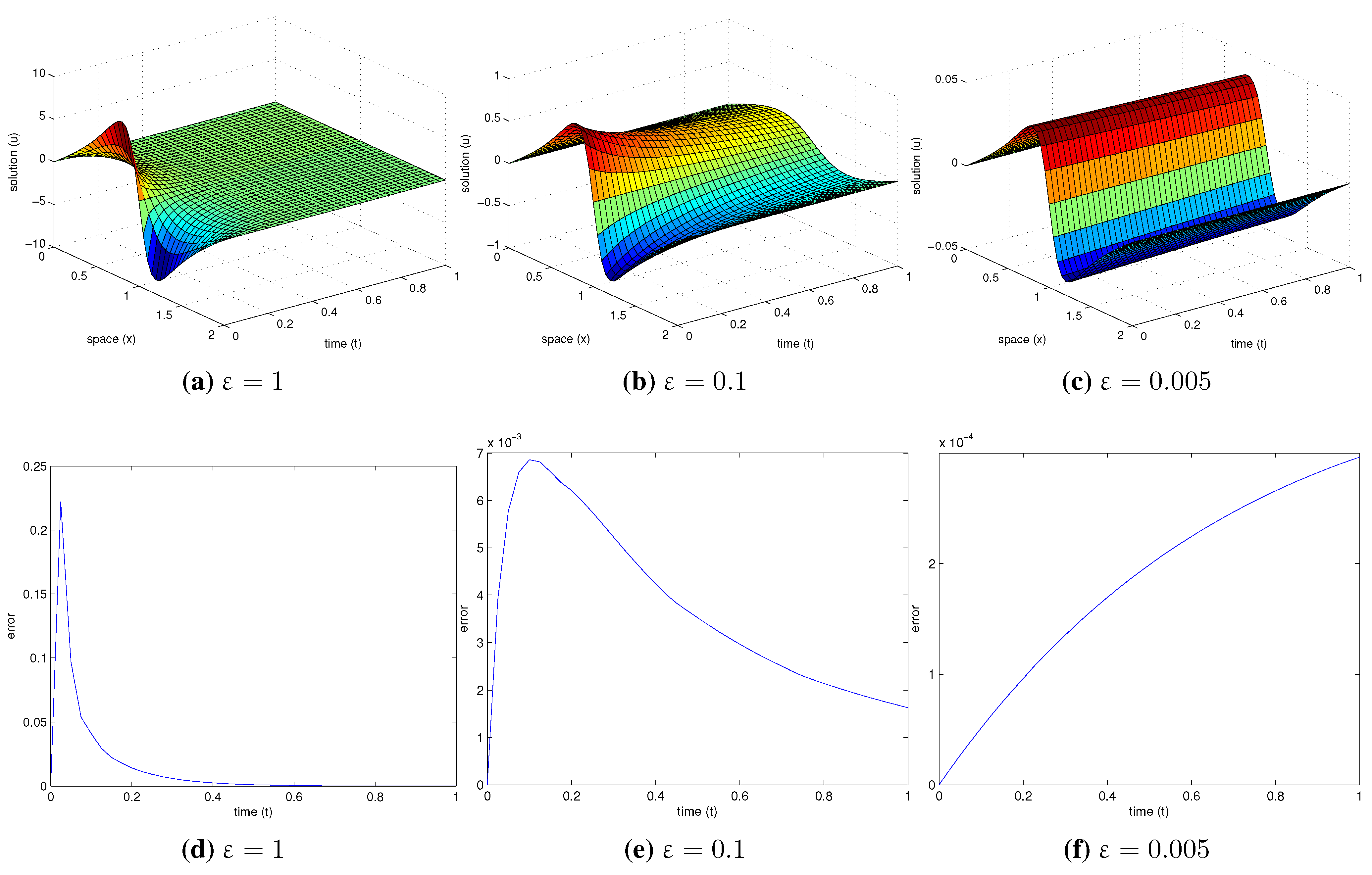
An interesting result emerges from that error matrix if we consider a sufficiently high upper bound of the studied time. If we obtain the GE between all values of
x on each time we observe that the GE increase really fast at first but after the peak is reached it starts to decrease. This result can be seen on the
Figure 1.
In
Table 1 we set the maximum time of the study, the number of time nodes and the Reynolds constant as
,
and
and we try different amount of space nodes. In each case we obtain the already mentioned GE and the average number of iterations (Avg. iter.) needed to solve each nonlinear system by using Newton’, Traub’s and M5 methods.
From these results we observe that, in general, the more space subintervals we take (smaller space step), the less is GE.
In
Table 2, we repeat the same process but in this case we set the number of space nodes and try different amount of time nodes. So
,
and
.
As we can observe, at first it seems that the more time subintervals we take, the less is GE (similarly as it happened with the previous table, where we tried different amount of space subintervals) however there is a limit for this which if we exceed the error starts to increase again. In this case, the minimum error is obtained for .
Figure 1.
Solution (a–c) and error progression curve (d–f) for different times and ε values, with and .
Figure 1.
Solution (a–c) and error progression curve (d–f) for different times and ε values, with and .
Table 1.
Comparison of the GE (greatest error) and methods iterations for different amount of space subintervals.
Table 1.
Comparison of the GE (greatest error) and methods iterations for different amount of space subintervals.
| | | | | | |
|---|
| Greatest error | 0.09033 | 0.029932 | 0.0070658 | 0.0017149 | 0.00039376 |
| Avg. iter. Newton | 4 | 4 | 4 | 4 | 4 |
| Avg. iter. Traub | 3 | 3 | 3 | 3 | 3 |
| Avg. iter. M5 | 3 | 3 | 3 | 3 | 3 |
Table 2.
Comparison of the GE and methods iterations for different amount of time subintervals.
Table 2.
Comparison of the GE and methods iterations for different amount of time subintervals.
| | | | | | |
|---|
| Greatest error | 0.0043069 | 0.00015291 | 0.00083542 | 0.0010565 | 0.0011128 |
| Avg. iter. Newton | 4.4 | 4.15 | 4 | 4 | 4 |
| Avg. iter. Traub | 3.4 | 3.1 | 3 | 3 | 3 |
| Avg. iter. M5 | 3 | 3 | 3 | 3 | 3 |
In
Table 3, we repeat the process again, however now we study the effect of choosing a small, regular or big value of the Reynolds constant (
), although we actually use
for simplicity. For doing this, we set the number of space and time nodes and the maximum time of study, so
,
and
.
Table 3.
Comparison of the GE and methods iterations for different values of ε.
Table 3.
Comparison of the GE and methods iterations for different values of ε.
| | | | | | | | |
|---|
| Greatest error | 0.22216 | 0.0068572 | 0.0035207 | 0.0021242 | 0.0014188 | 0.000708 | 0.000296 |
| Avg. iter. Newton | 3.9 | 4 | 4 | 4 | 4 | 3.85 | 3 |
| Avg. iter. Traub | 3.15 | 3 | 3 | 3 | 3 | 3 | 3 |
| Avg. iter. M5 | 2.8 | 3 | 3 | 3 | 3 | 3 | 2 |
First of all, it has to be said that the maximum value of ε that can be used to keep the method working properly will depend of the amount of time subintervals we take, it happens because the bigger is the attenuation, more abrupt are the curves on the time axis. For keeping the error low, a finer mesh will be needed, what can be obtained by increasing the amount of time subintervals. From
Table 3 we can numerically see this phenomenon, for a fast attenuation (
) the error is quite big due to the curve is very abrupt (as we said we could decrease the error of this case by taking more time subintervals), however the slower is the attenuation (lower values of ε), lower is GE. If we keep on taking lower values of attenuation (lower ε), the peak of the GE characteristic curve will not be reached and consequently the GE will be even lower (for this example it happens for
and even more for
). See
Figure 1 for a better understanding of these different situations.
Some conclusions can be obtained from
Table 1,
Table 2 and
Table 3: to use a higher order method (like M5) does not represent a bigger advantage compared with a typical third order method (like Traub), however there is a significant difference between using a third order method compared to a typical second order method (like Newton). The more space subintervals we take, lower is GE; however, it does not happen with the amount of time subintervals, it means that there is an optimum amount of time subintervals that reduces the GE to its minimum but after it the error starts to increase again and the computational cost of having to solve so many systems does not make any sense (due to the increasing number of floating points operations, execution time,...). As we have seen from
Table 3, if we want to study a situation with a big attenuation (low
), we will need a higher amount of time subintervals compared to those situations where the attenuation is lower (it means that the computational cost for having to solve more nonlinear systems will be higher), however taking more space subintervals does not seem to help.
Example 2. Let us consider now the following initial and boundary conditions for Burgers’ equation
and
.
In
Figure 2 we see a plot of the approximated solution by our method at different times for
and for two different values of ε, and in
Table 4 we show the numerical results of this solution for some values of
and ε.
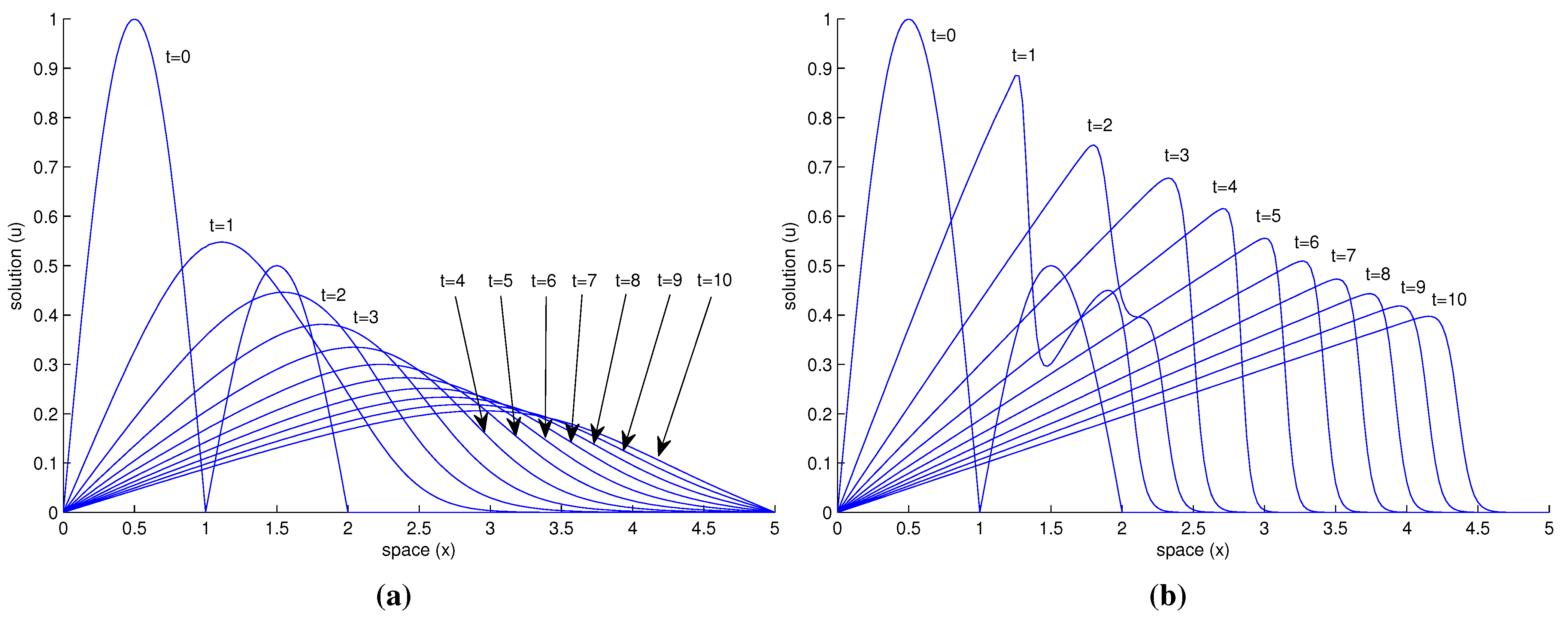
Figure 2.
Solution for different times and ε values, both of them with and . (a) ; (b) .
Figure 2.
Solution for different times and ε values, both of them with and . (a) ; (b) .
Table 4.
Numerical results of the approximated solution for different values of and ε.
Table 4.
Numerical results of the approximated solution for different values of and ε.
| x | t | | |
|---|
| 1.5 | 2 | 0.44533 | 0.63548 |
| | 4 | 0.28961 | 0.34573 |
| | 6 | 0.20701 | 0.23678 |
| | 8 | 0.16020 | 0.17999 |
| | 10 | 0.13041 | 0.14516 |
| 3 | 2 | 0.02972 | 0.00000 |
| | 4 | 0.14900 | 0.00470 |
| | 6 | 0.22312 | 0.47269 |
| | 8 | 0.22501 | 0.35971 |
| | 10 | 0.20562 | 0.29021 |
| 4.5 | 2 | 0.00001 | 0.00000 |
| | 4 | 0.00145 | 0.00000 |
| | 6 | 0.01171 | 0.00000 |
| | 8 | 0.03557 | 0.00000 |
| | 10 | 0.06242 | 0.02066 |
This results are very similar to those obtained for Mittal and Singhal on their paper (see [
12]), where they transform Burgers’ equation into a system of nonlinear ordinary differential equations and solve it by Runge-Kutta-Chebyshev second order method. Although the techniques used to solve the problem are different, the results obtained by Mittal-Singhal and ours, showed in
Table 4 and
Figure 2 have the same order of magnitude. As we can see in
Figure 2 it happens indeed that the lower is ε, slower is the attenuation. Although in this example we have used a piecewise initial condition, and it usually brings more problems, we still have obtained satisfactory results. Since we have considered a quite high upper bound of the studied time (
) we have had to take a bigger value of
m in order to keep a fine mesh size. The results obtained in both
Figure 2 and
Table 4 are the same regardless if we use Newton’, Traub’s or M5 method.


