An Introduction to Clique Minimal Separator Decomposition

Abstract

This paper is a review which presents and explains the decomposition of graphs by clique minimal separators. The pace is leisurely, we give many examples and figures. Easy algorithms are provided to implement this decomposition. The historical and theoretical background is given, as well as sketches of proofs of the structural results involved.

1. Introduction

This paper is designed as a presentation for the not so well-known graph decomposition which we call “clique minimal separator decomposition”. In view of recent applications, this decomposition is a promising tool.

A separator is a set of vertices (of a connected graph), the removal of which disconnects the graph, and a clique is a set of pairwise adjacent vertices, and of course a clique separator is a separator which is a clique. Clique minimal separator decomposition is a process which breaks up an undirected graph into a set of subgraphs by copying the clique minimal separators into the connected components they define, as will be explained in detail further.

Historically, clique separator decomposition was studied by graph theorists because some hard graph problems such as vertex coloring, maximum clique and testing for perfection can be solved by a Divide-and-Conquer approach by first solving them on the subgraphs defined by a clique separator decomposition, and then merging the obtained results.

There are two main drawbacks to this decomposition:

• First, not every graph has a clique separator.
• Second, the subgraphs obtained are not disjoint, which means that if the overlap is large, little is to be gained by a Divide-and-Conquer approach.

However, recent research has modelized data by graphs (such as text mining data [1], biochip data [2], or any data represented by a symmetric positive matrix such as distance data). In those graphs, a clique is often an important locus, since it reflects maximum interaction between its elements. These graphs almost always have clique separators. But in any case, when these graphs are obtained by choosing a threshold in a distance matrix, one can choose a threshold which defines a graph which contains a sufficient number of clique separators.

The fact that the subgraphs obtained overlap can be a desirable property in applications. For example, when searching for clusters of genes, it is nice to be able to allow a gene to interact with different gene groups, which is not the case with classical gene clustering.

The theory of clique decomposition and clique minimal separator decomposition has been studied by several authors. The mathematical baggage necessary to prove the results we present here is somewhat complicated, and the results are distributed between various papers, which is one of the reasons for which this graph decomposition is not as well-known as it could be. We will describe the known results (while citing the corresponding reference papers when possible). We also devote a section to giving the proof (or at least a sketch of proof) of the main results we use.

Our aim in this paper is to explain this decomposition as simply as possible; the basic process is not difficult to understand, and it is not difficult to implement. However, it does involve some not so easy graph notions such as minimal separation. We have organized the results so that graph theorists will find the theoretical background, and so that scientists from other areas can use and implement this decomposition, by giving examples and explaining the implementations.

The paper is organized as follows:

• Section 2 gives some general graph notions, some particulars on minimal separation and minimal triangulation.
• Section 3 provides a precise definition of clique minimal separator decomposition, as well as examples; we also discuss how to find the clique minimal separators of a graph efficiently, and give some properties of this decomposition.
• Section 4 gives an efficient process for computing the clique minimal separator decomposition of a graph.
• Section 5 provides a brief history of clique decomposition, with the bibliographic background as well as high-level proofs of the results we present in this paper.
• We conclude in Section 6.

2. Graph Notions

2.1. General notions

All graphs in this work are undirected and finite. A graph $G=(V,E)$ is a set V of vertices, $\left|V\right|=n$, and a set E of edges which are pairs of distinct vertices, $\left|E\right|=m$; an edge $\{x,y\}$ is denoted $xy$. The complement $\overline{G}=(V,\overline{E})$ of graph $G=(V,E)$ is the graph where, for any pair of vertices $\{x,y\},x\ne y$, edge $xy\in \overline{E}$ if and only if $xy\notin E$. If $X\subset V$ is a set of vertices of $G=(V,E)$, $G\left(X\right)$ denotes the subgraph induced by X (which is a graph whose vertices are the elements of X and such that $xy$ is an edge of $G\left(X\right)$ if $x,y\in X$ and $xy\in E$).

Neighborhoods: 

The neighborhood of a vertex x in G is $N_G\left(x\right)=\{y\ne x\mid xy\in E\}$; we omit subscript G when it is clear from the context which graph we work on. The extended neighborhood of a vertex x is $N_G\left[x\right]=N_G\left(x\right)\cup \left\{x\right\}$. We say that vertices x and y are adjacent if and only if $xy\in E$. The neighborhood of a set of vertices A is $N_G\left(A\right)={\cup }_{x\in A}{N}_G\left(x\right)-A$, and its extended neighborhood is $N_G\left[A\right]=N_G\left(A\right)\cup A$.

Paths and cycles:

A path is a sequence $(x_1,x_2,\dots ,x_k)$ of different vertices such that for $i<k$, $x_i$ is adjacent to $x_{i+1}$. A chord in a path is an edge $x_i{x}_j$ where $j>i$ and $j\ne i+1$. A path is chordless if it has no chord. A cycle is a “closed path”, i.e., a sequence $x_1,x_2,\dots ,x_k,x_1$ of vertices, with $x_1,x_2,\dots ,x_k$ all different, such that for $i<k$, $x_i$ is adjacent to $x_{i+1}$ and $x_k$ is adjacent to $x_1$. A chordless cycle is a cycle with no chord. A chordless cycle with 5 or more vertices is called a hole, the complement of such a cycle is called an antihole.

Connexity: 

A graph is connected if there is a path connecting any pair of vertices, disconnected otherwise ; when the graph is disconnected, the maximal connected subgraphs are called the connected components of the graph.

Cliques: 

A clique is a set of vertices which are pairwise adjacent. An independent set is a set of vertices with no edges.

Perfection: 

A graph is perfect if it contains no induced hole or antihole with an odd number of vertices.

Example 2.1

In Figure 1, $(a,b,c,k)$ is a chordless cycle of length 4, $\{c,d,j,k\}$ is a clique, $N\left(c\right)=\{b,d,j,k\}$, $N\left(\right\{a,b\left\}\right)=\{c,k\}$.

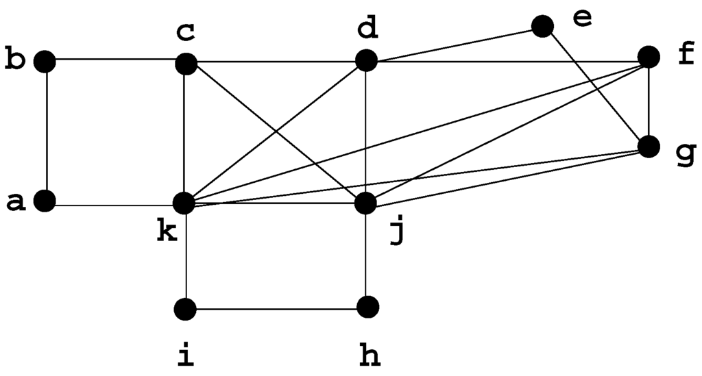
Figure 1. Graph G, our running example.

Figure 1. Graph G, our running example.

2.2. Minimal separation, chordal graphs, and minimal triangulation

Definition 2.2

• A subset S of vertices of a connected graph G is called a separator (or sometimes a cutset) if $G(V-S)$ is not connected.
• A separator S is called an $ab$-separator if a and b lie in different connected components of$G(V-S)$, a minimal $ab$-separator if S is an $ab$-separator and no proper subset of S is an $ab$-separator.
• A separator S is a minimal separator, if there is some pair $\{a,b\}$ such that S is a minimal $ab$-separator.

Alternately, S is a minimal separator if and only if $G(V-S)$ has at least 2 connected components $C_1$ and $C_2$ such that $N\left(C_1\right)=N\left(C_2\right)=S$; such components are called full components of S in G. S is a minimal $xy$-separator for any $\{x,y\}$ with $x\in C_1$ and $y\in C_2$.

A connected graph with no minimal separator is a clique.

When the graph is not connected, the set of minimal separators is the union of the sets of minimal separators of the connected components.

Example 2.3

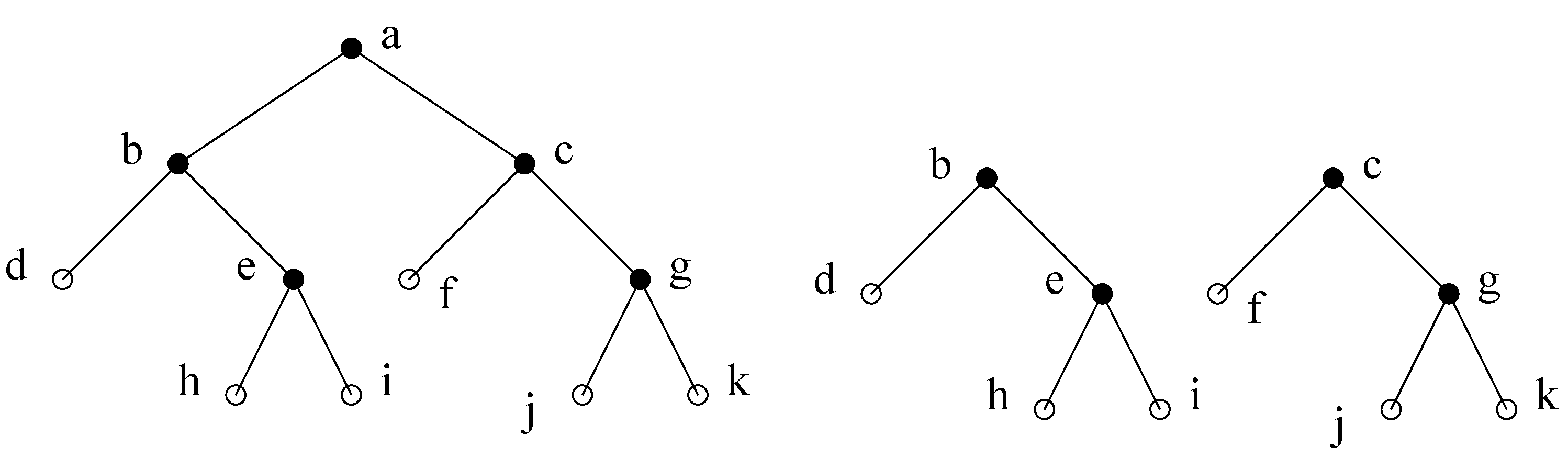
Let us illustrate these notions on a tree: a tree has two kinds of vertices: leaves and articulation nodes (which are its minimal separators). Figure 2 shows how removing articulation node $\left\{a\right\}$ disconnects the graph into several connected components; $\left\{a\right\}$ is a $df$-separator, as d and f lie in two different components.

Figure 2. $\left\{a\right\}$ is a $df$-separator. 

Figure 2. $\left\{a\right\}$ is a $df$-separator. 

Example 2.4

On the more complex graph G of Figure 1: $\{c,d,j,k\}$ is a separator, but it is not minimal. $\{d,j,k\}$ is a minimal separator, with full components $\{a,b,c\}$ and $\{e,f,g\}$. $\{j,k\}$ is also a minimal separator, with full components $\{h,i\}$ and $\{a,b,c,d,e,f,g\}$. Note that minimal separator $\{j,k\}$ is included in minimal separator $\{d,j,k\}$.

Note that in an arbitrary graph, there can be an exponential number of minimal separators $\left(O\left(2^n\right)\right)$. Figure 3 shows an example of this.

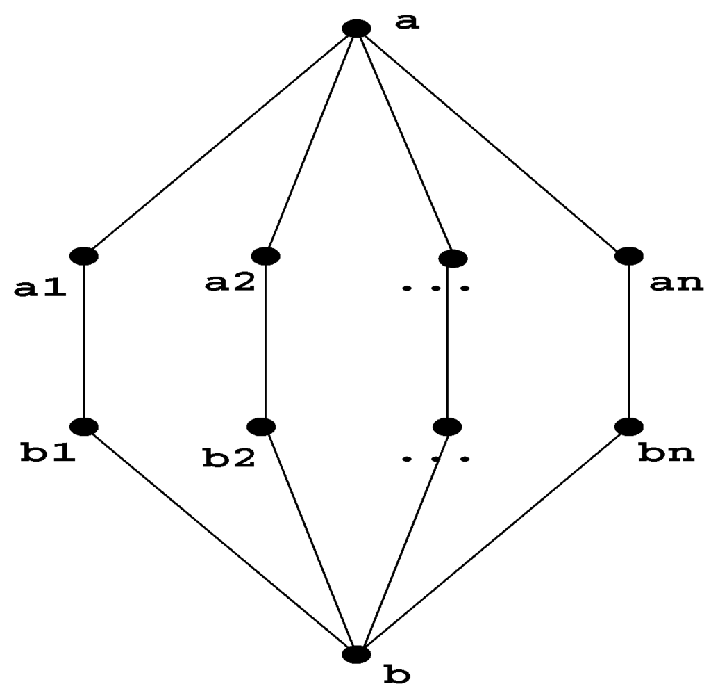
Figure 3. This graph has an exponential number of minimal separators, which are the combinations from the Cartesian product $\{a_1,b_1\}\times \{a_2,b_2\}\times \dots \times \{a_n,b_n\}$.

Figure 3. This graph has an exponential number of minimal separators, which are the combinations from the Cartesian product $\{a_1,b_1\}\times \{a_2,b_2\}\times \dots \times \{a_n,b_n\}$.

Chordal graphs:

A graph is chordal if it has no chordless cycle of length strictly greater than 3; chordal graphs are extensions of trees and have many similar properties. Dirac [3] originally defined the concept of a minimal separator in order to characterize chordal graphs, by showing that a graph G is chordal if and only if every minimal separator of G is a clique. In a chordal graph, there are less than n minimal separators [4]. Figure 4 shows a chordal graph H.

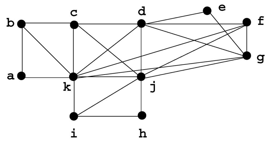
Figure 4. Chordal graph H, with minimal separators: $\{b,k\},\{c,k\},\{d,j,k\},\{j,k\},\{i,j\},$ $\{d,g\}.$

Figure 4. Chordal graph H, with minimal separators: $\{b,k\},\{c,k\},\{d,j,k\},\{j,k\},\{i,j\},$ $\{d,g\}.$

Perfect elimination orderings:

Another interesting characterization of chordal graphs is that they have a simplicial ordering on the vertices: a vertex is said to be simplicial if its neighborhood is a clique. A graph is chordal if and only if one can repeatedly find a simplicial vertex, and remove it, until no vertex is left. Since at each step a vertex is removed, this defines a series of transitory graphs: at step $i+1$, the transitory graph is input graph G from which the first i vertices have been removed. This process is called a simplicial elimination scheme, and defines an ordering on the vertices called a perfect elimination ordering (peo).

Each minimal separator of a chordal graph H is the neighborhood of a vertex in the transitory graph in the simplicial elimination scheme [4]. We will say that such a vertex generates a minimal separator of H (w.r.t. a given peo of H):

Definition 2.5

Let $H=(V,E)$ be a chordal graph, let α be a perfect elimination ordering of H. We say that vertex x of number i by α generates minimal separator S w.r.t α if S is equal to the set of neighbors of x of higher number.

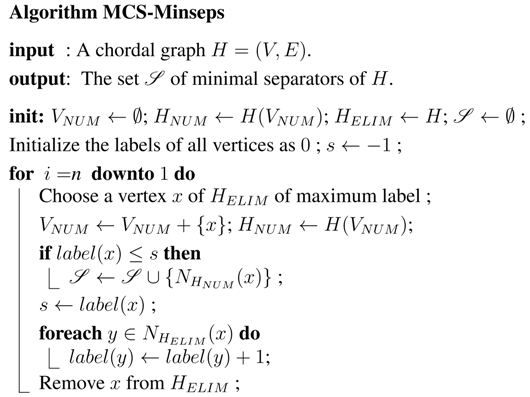
Thus, to compute the set of minimal separators of H, it is sufficient to compute a peo α of H and to select the vertices that generate a minimal separator of H w.r.t. α. This is easy to accomplish with a special kind of peo defined by algorithms such as MCS [5], and will be used for our implementation in Section 4.

Minimal triangulations: 

A triangulation is a chordal completion of a graph: a set F of edges (called the fill edges)is added to the graph in order to obtain a chordal graph.

Definition 2.6

Let $G=(V,E)$ be a graph. A chordal graph $H=(V,E+F)$ is called a triangulation of G, and F is called the fill. The triangulation is said to be:

• minimal if for no proper subset $F^{\prime }$ of F, $H^{\prime }=(V,E+F^{\prime })$ is chordal.
• minimum if no other minimal triangulation has less fill edges.

Example 2.7

Graph H from Figure 4 is a minimal triangulation of Graph G from Figure 1 (see Figure 5).

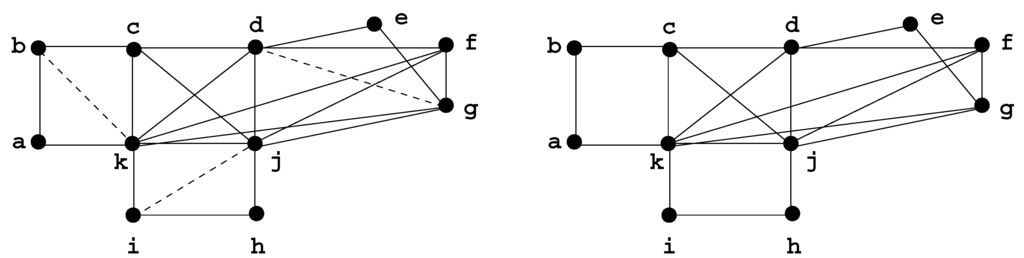
Figure 5. H is a minimal triangulation of G. The fill edges are represented by dotted lines.

Figure 5. H is a minimal triangulation of G. The fill edges are represented by dotted lines.

Computing a minimum triangulation is NP complete [6], but computing a minimal triangulation can be done in $O\left(nm\right)$ time (or a little less for dense graphs [7,8]). This problem has given rise to several recent papers, so there are now many minimal triangulation algorithms (see e.g. [9,10,11,12]). We will use one of them (MCS-M) in Section 4 where we describe an implementation.

Minimal elimination orderings:

One way to compute a triangulation of a graph $G=(V,E)$ is to force the graph into having a perfect elimination ordering: define an ordering α on V, repeatedly pick the next vertex by α, add any edges missing in its neighborhood (in the subgraph induced by the not yet removed vertices), and remove it, until no vertex is left. This will yield a triangulation $G_{\alpha }^{+}=(V,E+F)$ whose fill F is the set of all edges added in this process.

An ordering α on the set of vertices of G is a minimal elimination ordering (meo) of G if the triangulation $G_{\alpha }^{+}$of G obtained is a minimal triangulation of G.

Algorithm LEX M [13] was devised to compute an meo. In Section 4, we will use a simpler version of LEX M, MCS-M [9]. Both these algorithms yield a minimal triangulation H of the input graph G and an ordering α that is both a meo of G and a peo of H, and makes it easy to compute the set of vertices generating the minimal separators of H.

3. Defining clique minimal separator decomposition

3.1. Definitions and examples

The decomposition by clique minimal separators can be defined by the following algorithmic process on input graph G: define a collection of subgraphs (which at the beginning contains only G) by repeatedly applying the following decomposition step on a subgraph which has a clique minimal separator, until none of the subgraphs has a clique minimal separator.

Decomposition Step 3.1

Given a graph $G^{\prime }$, find a clique minimal separator S of $G^{\prime }$ and a full component C of S; replace $G^{\prime }$ with the following 2 subgraphs: $G_1=G^{\prime }(S\cup C)$, $G_2=G^{\prime }(V-C)$.

The decomposition is the set of subgraphs obtained in the end, which are called atoms.

The decomposition is unique, the resulting set of atoms does not depend of the order in which the decomposition steps are executed. This is because of the following property of clique minimal separator decomposition:

Property 3.2

Let $\mathcal{S}$ be the set of minimal separators of a graph $G^{\prime }$, let S be a clique minimal separator of $G^{\prime }$; after application of one decomposition Step 3.1, each other minimal separator is a minimal separator of either $G_1^{\prime }$ or of $G_2^{\prime }$.

Thus in particular, any clique minimal separator will be a clique minimal separator of $G_1$ or of $G_2$. Note that the clique minimal separator which was used, S, may or may not still be a minimal separator of $G_2$, depending on whether S had more than two or only two full components.

The atoms obtained are characterized as follows:

Characterization 3.3

An atom of graph G is a maximal connected subgraph containing no clique minimal separator.

Example 3.4

• Figure 6 gives the decomposition of a tree.
• On any chordal graph, this decomposition yields the set of maximal cliques of the input graph.
• In a non-chordal graph, some of the atoms will not be cliques. Let us use our graph G from Figure 1 as an example: The clique minimal separators of G are: $\{c,k\}$, {j,k}$,\{d,j,k\}$. Figure 7 shows a decomposition tree and the set of atoms.

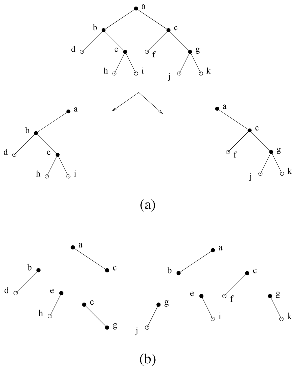
Figure 6. (a) A decomposition step using minimal separator $\left\{a\right\}$. The minimal separators (except for $\left\{a\right\}$) are partitioned into the two subtrees obtained. (b) Total decomposition.

Figure 6. (a) A decomposition step using minimal separator $\left\{a\right\}$. The minimal separators (except for $\left\{a\right\}$) are partitioned into the two subtrees obtained. (b) Total decomposition.

3.2. Properties of the atoms

• The number of atoms is at most n.
• The intersection between atoms is always a clique (which may be empty), and it is not necessarily a minimal separator (even when it is not empty).

Example 3.5

In our example from Figure 7, atom $\{a,b,c,k\}\cap$ atom $\{c,d,j,k\}=\{c,k\}$, which is not a minimal separator; atom $\{a,b,c,k\}\cap$ atom $\{i,j,k,h\}=$$\{j,k\}$, a minimal separator.

3.3. An equivalent process

Another way of doing the decomposition is using a clique minimal separator S and copying it in all the components it defines. For a component C which is not a full component, we need to copy only the neighborhood of C. This corresponds to a clique minimal separator which is properly included in S.

The property we use is the following:

Property 3.6

Let S be a minimal separator, let $\left(C_i\right)$ be connected components of $G(V-S)$. Then $\forall i$, $N_G\left(C_i\right)$ is a minimal separator of G.

Figure 7. A decomposition tree for graph G from Figure 1 and the set of atoms of G.

Figure 7. A decomposition tree for graph G from Figure 1 and the set of atoms of G.

This leads to the following decomposition step:

Decomposition Step 3.7

Given a graph $G^{\prime }$ with a clique minimal separator S, let $C_1,\dots ,C_k$ be the connected components of $G^{\prime }(V-S)$. Replace $G^{\prime }$ with the subgraphs $G^{\prime }(C_i\cup N_{G^{\prime }}\left(C_i\right))$.

After such a decomposition step using clique minimal separator S, S and the clique minimal separators subsets of S can no longer be a minimal separator in any of the subgraphs obtained, and all the other minimal separators of G are partitioned into the subgraphs obtained.

Example 3.8

Figure 8 shows a decomposition step in graph G from Figure 1 using Decomposition Step 3.7.

An application of Decomposition Step 3.7 corresponds to several applications of Decomposition Step 3.1.

3.4. How to compute the clique minimal separators

To our knowledge, the only efficient known way to compute the clique minimal separators of a graph is to extract them from a minimal triangulation.

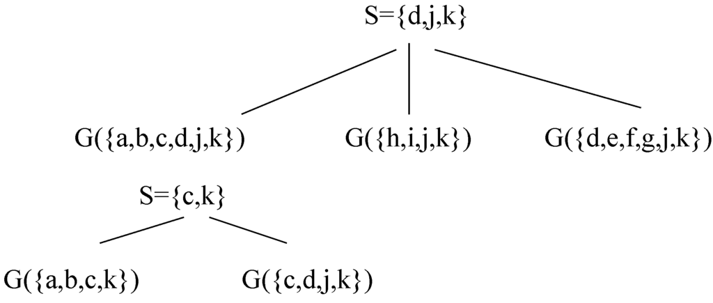
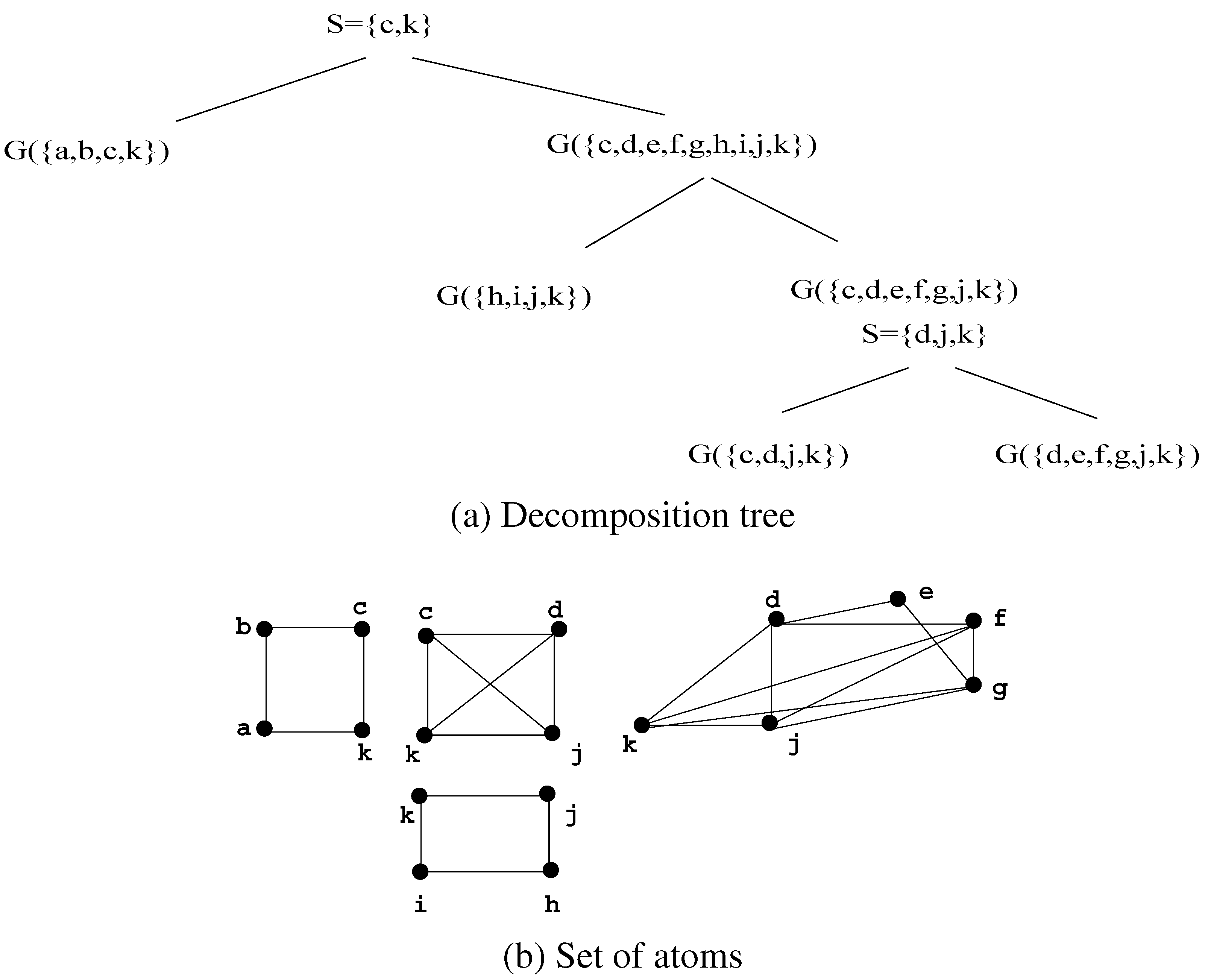
Figure 8. A decomposition of G using Decomposition Step 3.7.

Figure 8. A decomposition of G using Decomposition Step 3.7.

This method is based on the following property:

Property 3.9

Let $G=(V,E)$ be a graph, let $H=(V,E+F)$ be a minimal triangulation of G. The clique minimal separators of G are exactly the minimal separators of H that are cliques in G.

Thus in order to find the clique minimal separators of a graph, the general process is as follows:

• compute a minimal triangulation H of G.
• compute the minimal separators of H.
• check each minimal separator of H to see whether it is a clique in G.

Computing the minimal separators of a minimal triangulation of a graph can be done efficiently using an ordering provided by a search algorithm such as MCS-M, and Steps 1 and 2 can be merged, as we will see in Section 4.

Example 3.10

Graph H from Figure 4 is a minimal triangulation of Graph G from Figure 1. The minimal separators of H are: $\{b,k\},\{c,k\},\{d,j,k\},\{j,k\},\{i,j\},\{d,g\}$. Three of them are cliques in G: $\{c,k\},\{d,j,k\},\{j,k\}$, so they are clique minimal separators of G.

3.5. Some problems which can be solved using the atoms

• Minimal and minimum triangulation: if a minimal triangulation is computed for each of the atoms of the clique minimal separator decomposition of a graph, then the union of the set of fill edges obtained defines a minimal triangulation for G. Thus if for each atom a minimum-sized fill is computed, the resulting fill will be a minimum triangulation of G, since the sets of fill edges in the atoms are pairwise disjoint.
• Treewidth: the treewidth is obtained by taking the largest treewidth over all the atoms.
• Perfection: Any chordless cycle of length 4 or more is preserved by a decomposition step, as well as any antihole, so this decomposition preserves holes and antiholes. Thus a graph is perfect if and only if all its atoms are perfect.
• Coloring: An optimal coloring is obtained by merging optimal colorings of the atoms.
• Maximum clique: Any maximal clique of the graph is preserved after a decomposition step, so finding the size of the largest clique of each atom will yield the size of the largest clique of the original graph.

4. Algorithms and implementations

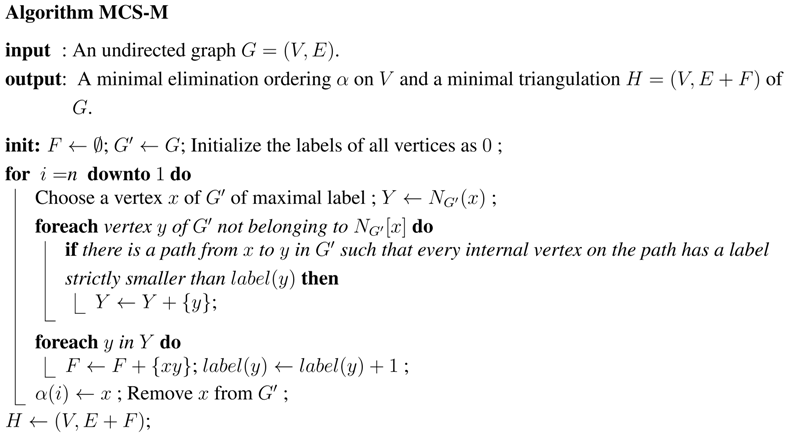
There are several ways of computing the decomposition of a graph into atoms. The simplest is to implement Decomposition Step 3.1. We will use Algorithm MCS-M [9], a search algorithm which computes a minimal triangulation $H=(V,E+F)$ of the input graph $G=(V,E)$, represented by a set F of fill edges, as well as an ordering α of the vertices. MCS-M numbers the vertices from n to 1, and the ordering α obtained is a meo of the input graph G and a peo of the minimal triangulation H which is computed [14].

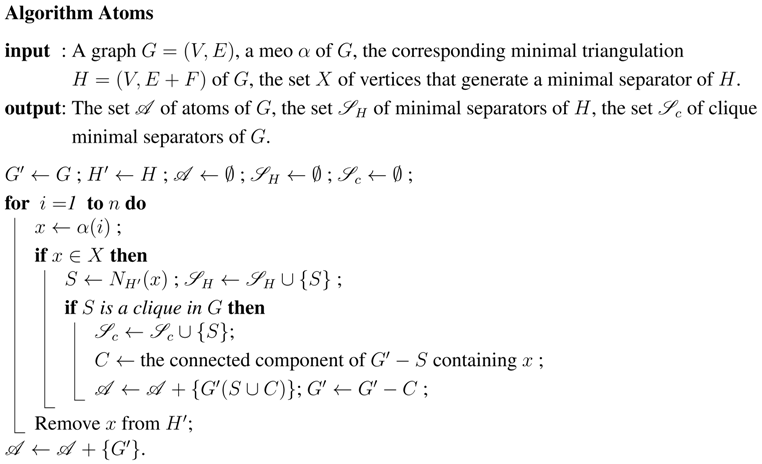
Once this ordering and this triangulation are computed, we will use them in a second algorithm, (Algorithm Atoms), which will generate the atoms by scanning the vertices from 1 to n.

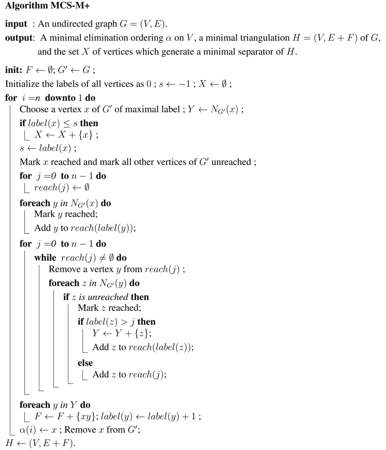
We will start by giving the general MCS-M algorithm, then an expanded version, which we call MCS-M+, as will be explained afterwards, and finally give the algorithm which yields the atoms.

$G^{\prime }$ will be the transitory subgraph of G induced by the set of still unnumbered vertices.

We will now expand this algorithm in two ways.

First, we will implement “if there is a path from x to y in $G^{\prime }$ such that every internal vertex on the path has a label strictly smaller than $label\left(y\right)$”.

We do this in a similar way as in the implementation of LEX M given in [13] by a single search in $G^{\prime }$. For each label value j, set $reach\left(j\right)$ contains the reached vertices having label j, as well as the vertices having a label strictly smaller than j reached from a vertex having label j.

Second, we will compute the set X of vertices that generate the minimal separators of the triangulation H, as described in [5]. The idea behind this is that as long as the labels of the chosen vertices keep getting larger, we are inside a clique of H; when suddenly the label of the chosen vertex x stops getting larger, x generates a minimal separator of H. Each such vertex x is added to set X.

Once we have obtained an MCS-M ordering α, as well as the corresponding minimal triangulation H of G and the set X of generators of the minimal separators of H, we run through the vertices from 1 to n. We use the transitory subgraphs $G^{\prime }$ and $H^{\prime }$ of G and H, initialized as G and H, respectively. At each step i processing vertex $x=\alpha \left(i\right)$, we check whether x is in the set X. If it is, the neighborhood $N_{H^{\prime }}\left(x\right)$ of x in $H^{\prime }$ is a minimal separator of H; we check whether it is a clique in G. If it is, then S is a clique minimal separator of G. In that case we compute the connected component C of $G(V-S)$ which contains x; $G^{\prime }(S\cup C)$ is an atom [15], and is stored as such; C is then removed from $G^{\prime }$. In any case, we then remove x from $H^{\prime }$.

5. Theoretical and bibliographical background

5.1. A brief history of clique minimal separator decomposition

In 1976, Gavril [16] described the class of “clique separable graphs” in the context of solving in polynomial time the hard problems of minimum coloring and maximum clique.

In 1980, the problem of finding a clique separator in an arbitrary graph was addressed by Whitesides [17], who presented an $O\left(n^3\right)$ algorithm to find one clique separator.

In 1983, Tarjan [15] addressed the problem of finding a decomposition of an arbitrary graph using its clique separators. He noted that using Whitesides’ algorithm, this would require $O\left(n{m}^3\right)$ time. He proposed an $O\left(nm\right)$ time algorithm to do this, by showing that no fill edge of a minimal triangulation can join two connected components defined by a clique separator. Computing an meo required $O\left(nm\right)$ time, as he showed in [13] (1976), and he proved that using an meo, a clique separator decomposition can be computed in $O\left(nm\right)$ time. Tarjan left open the question of defining a unique clique separator decomposition.

In 1990, Dahlhaus, Karpinsky and Novick [18] proposed a parallel algorithm for clique separator decomposition.

In 1990, concurrently, Leimer [19], in a paper sent out for publication in 1986, described in every mathematical detail how to obtain an optimal and unique decomposition using the clique minimal separators of the graph. Leimer also described how to use LEX M (also called the RTL algorithm) to find a clique minimal separator decomposition in $O\left(nm\right)$ time.

In 2001, Olesen and Madsen [20] applied clique minimal separator decomposition to Bayesian networks, and presented an approach based on the clique tree of a minimal triangulation to compute the atoms (which they call maximal prime subgraphs) by merging in the clique tree any two nodes connected by an edge which represents a non-clique minimal separator (the reader is referred to [21] for full details on clique trees).

5.2. Computing the clique minimal separators of a graph

We first prove that for any graph G and any minimal triangulation H of G, the clique minimal separators of G are exactly the minimal separators of H that are cliques in G (property 3.9).

For this, it is sufficient to show that any clique of G has the same number of full components in G as in H. This follows from the following property, which is an extension of Lemma 1 from [15].

Property 5.1

Let $G=(V,E)$ be a graph, let $H=(V,E+F)$ be a minimal triangulation of G and let S be a clique of G. Then $G(V-S)$ and $H(V-S)$ have the same connected components, with the same neighborhoods.

Proof: 

Let $H^{\prime }$ be the graph defined by $H^{\prime }=(V,E+F^{\prime })$, where $F^{\prime }$ is the set of edges in F that are contained in $N_G\left[C\right]$ for some connected component C of $G(V-S)$. By definition of $H^{\prime }$, $G(V-S)$ and $H^{\prime }(V-S)$ have the same connected components, with the same neighborhoods. Let us show that $H^{\prime }$ is chordal. Let μ be a cycle in $H^{\prime }$ of length greater than 3, and let us show that μ has a chord in $H^{\prime }$. As H is chordal, μ has a chord, say $xy$, in H. If $xy$ is in $H^{\prime }$ then it is a chord of μ in $H^{\prime }$. Otherwise there is a connected component C of $G(V-S)$ such that x is in C and y is in $V-N_G\left[C\right]$, or conversely. Hence there are two non-consecutive vertices w and z of μ that are both in $N_G\left(C\right)$, and therefore both in clique S of $H^{\prime }$. It follows that $wz$ is a chord of μ in $H^{\prime }$, which completes the proof that $H^{\prime }$ is chordal. As $G\subseteq H^{\prime }\subseteq H$, with $H^{\prime }$ chordal and H a minimal triangulation of G, $H^{\prime }=H$, and therefore $G(V-S)$ and $H(V-S)$ have the same connected components, with the same neighborhoods. □

Corollary 5.2

(Property 3.9) Let $G=(V,E)$ be a graph, let $H=(V,E+F)$ be a minimal triangulation of G. The clique minimal separators of G are exactly the minimal separators of H that are cliques in G.

The fact that each minimal separator of a chordal graph H is generated by a vertex of H w.r.t. a peo of H [4] is well-known. A way of selecting the exact vertices that generate a minimal separator is discussed in [5].

The following algorithm is based on the expanded version of MCS presented in [21] to generate the maximal cliques and a clique tree.

This process is integrated in the implementation given in Section 4.

5.3. Decomposing a graph into atoms

Decomposition Step 3.1 and Algorithm Atoms of Section 4 are largely inspired from the decomposition of a graph by clique separators described by Tarjan [15]. Tarjan considers clique separators instead of clique minimal separators, with the drawback that the set of atoms obtained is not unique (see SubSection 5.4). He also computes a meo of G and the corresponding minimal triangulation of G, but he selects the vertices that generate a clique separator instead of a clique minimal separator of G. The proof of the clique separator decomposition algorithm given in [15] can easily be modified into a proof of Algorithm Atoms. We will give an idea of this proof.

Theorem 5.3

Algorithm Atoms computes a clique minimal separator decomposition of input graph G.

Proof: 

(idea of the proof) The proof works by induction on $k=|X^{\prime }|$, where $X^{\prime }$ is the set of vertices of X that generate a clique of G w.r.t. α, i.e., the set of vertices of G that generate a clique minimal separator of G w.r.t. α. If k = 0 then the computed decomposition is $\left\{G\right\}$, which is correct since G has no clique minimal separator. We suppose that the decomposition is correct if $|X^{\prime }|\le k$. Let us show that it is still correct if $|X^{\prime }|=k+1$. Let x be the first vertex of $X^{\prime }$ in ordering α, let S be the clique minimal separator of G generated by x w.r.t. α, let C be the connected component of $G(V-S)$ containing x, let $G_1=G(S\cup C)$ and $G_2=G(V-C)$. For j in $\{1,2\}$, let $V_j$ be the vertex set of $G_j$, let ${\alpha }_j$ be the restriction of α to $V_j$, let $H_j=H\left(V_j\right)$ and $X_j^{\prime }=X^{\prime }\cap V_j$. It can be shown that for j in $\{1,2\}$, ${\alpha }_j$ is a meo of $G_j$, with $H_j$ as corresponding minimal triangulation of $G_j$. Moreover, each vertex of $V_2$ generates the same set in $G_2$ w.r.t. ${\alpha }_2$ as in G w.r.t. α, which is a minimal separator of $H_2$ if and only if it is a minimal separator of H. Hence $X_2^{\prime }$ is exactly the set of vertices of $G_2$ that generate a a clique minimal separator of $G_2$ w.r.t. ${\alpha }_2$, with $|X_2^{\prime }|\le k$ since $X_2^{\prime }\subseteq X^{\prime }-\left\{x\right\}$. It follows by induction hypothesis that $G_2$ is correctly decomposed. It remains to show that $G_1$ is an atom of G. It can be shown that each vertex of $C-\left\{x\right\}$ precedes x in ordering α, and generates the same set in $G_1$ w.r.t. ${\alpha }_1$ as in G w.r.t. α, which is a minimal separator of $H_1$ if and only if it is a minimal separator of H. As no vertex of $C-\left\{x\right\}$ generates a clique minimal separator of G w.r.t. α (since x is the first vertex that does), no vertex of $C-\left\{x\right\}$ generates a clique minimal separator of $G_1$ w.r.t. ${\alpha }_1$ either. Now each vertex of $S\cup \left\{x\right\}$ generates a subset of S, which is not a separator of $G_1$, w.r.t. ${\alpha }_1$. Hence $G_1$ has no clique minimal separator, and is therefore an atom of G. □

5.4. The unicity of clique minimal separator decomposition

Tarjan [15] originally defined the decomposition step of a graph by a clique separator as follows:

Decomposition Step 5.4

Let S be a clique separator of $G^{\prime }=(V^{\prime },E^{\prime })$, let $(S,A,B)$ be a partition of $V^{\prime }$ such that no vertex in A is adjacent to a vertex in B. Replace $G^{\prime }$ by $G_1^{\prime }=G^{\prime }(S\cup A)$ and $G_2^{\prime }=G^{\prime }(S\cup B)$.

He remarked that the set of atoms obtained by repeatedly applying this decomposition step is not unique, giving a counterexample that is recalled in Figure 9, and left the problem of the unicity of the decomposition open. Leimer [19] solved this problem, showing that using clique minimal separators instead of clique separators ensures unicity of the decomposition (with the additional condition that each one of A and B contains a full component of S in $G^{\prime }$ in the case of Decomposition Step 5.4). We present some elements of the proof of this result, which is associated in [19] with proofs of more complex results which make it difficult for non-specialists to follow. We first recall some definitions given in [19].

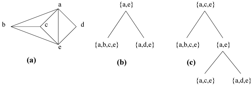
Figure 9. A graph with different decompositions by clique separators. (a) Graph. (b) One decomposition, which is the unique decomposition by clique minimal separators. (c) Another decomposition.

Figure 9. A graph with different decompositions by clique separators. (a) Graph. (b) One decomposition, which is the unique decomposition by clique minimal separators. (c) Another decomposition.

Definition 5.5

A graph is prime if it is connected and has no clique separator (or equivalently, no clique minimal separator). A mp-subgraph of a graph G is a maximal prime subgraph of G.

Leimer proved that the clique minimal separator decomposition of a graph G is the set of mp-subgraphs of G (Characterization 3.3). The proof of this characterization relies on the following property.

Property 5.6

Let $G=(V,E)$ be a graph, let S be a clique of G having at least one full component in G. Then there is a subset A of V such that $S\subset A$ and $G\left(A\right)$ is prime.

Proof: 

(idea of the proof) The property holds if G is chordal since in that case, as S is a clique of G having a full component, say C, in G, there is a vertex x of C such that $S\subseteq N_G\left(x\right)$ (this follows from the results in [4]), and therefore $S\cup \left\{x\right\}$ is a clique and induces a prime graph.

Let us show that it holds for any graph G. Let $G^{*}$ be the graph obtained from G by making each mp-subgraph of G into a clique. $G^{*}$ is chordal and has the same mp-subgraphs as G [19]. There is a subset A of V such that $S\subset A$ and $G^{*}\left(A\right)$ is prime. Let B be a subset of V such that $A\subseteq B$ and $G^{*}\left(B\right)$ is a mp-subgraph of $G^{*}$. Then $S\subset B$ and $G\left(B\right)$ is prime. □ He also showed the following characterization, which is Characterization 3.3:

Characterization 5.7 

The clique minimal separator decomposition of graph G is the set of mp-subgraphs of G.

Proof: 

We suppose that the decomposition step which is used is Decomposition Step 5.4 with the additional condition that each one of A and B contains a full component of S in $G^{\prime }$, which is more general than Decomposition Step 3.1.

The proof goes by induction on the number n of vertices of the graph. The property trivially holds if $n=1$. Suppose that it holds for any graph with at most n vertices. Let us show that it holds for a graph $G=(V,E)$ with $n+1$ vertices.

The property trivially holds if G has no clique minimal separator. We suppose that G has a clique minimal separator S. Let $(S,A,B)$ be a partition of V such that no vertex in A is adjacent to a vertex in B and each one of A and B contains a full component of S in G. Let $G_1=G(S\cup A)$ and $G_2=G(S\cup B)$. Let us show that the set $atoms\left(G\right)$ of atoms obtained by replacing G by $G_1$ and $G_2$ and further decomposing $G_1$ and $G_2$ is equal to the set $mp$-$subgraphs\left(G\right)$ of mp-subgraphs of G. Clearly $atom\left(G\right)=atoms\left(G_1\right)\cup atoms\left(G_2\right)$. As by induction hypothesis $atoms\left(G_1\right)=mp$-$subgraphs\left(G_1\right)$ and $atoms\left(G_2\right)=mp$-$subgraphs\left(G_2\right)$, it is sufficient to show that $mp$-$subgraphs\left(G\right)=mp$-$subgraphs\left(G_1\right)\cup mp$-$subgraphs\left(G_2\right)$.

Let us first show that $mp$-$subgraphs\left(G\right)\subseteq mp$-$subgraphs\left(G_1\right)\cup mp$-$subgraphs\left(G_2\right)$. Let $G\left(M\right)$ be in $mp$-$subgraphs\left(G\right)$. Then $M\subseteq S\cup A$ or $M\subseteq S\cup B$ (otherwise $M\cap S$ would be a clique separator of $G\left(M\right)$) and therefore $G\left(M\right)\in mp$-$subgraphs\left(G_1\right)\cup mp$-$subgraphs\left(G_2\right)$.

Let us show now that $mp$-$subgraphs\left(G_1\right)\cup mp$-$subgraphs\left(G_2\right)\subseteq mp$-$subgraphs\left(G\right)$. Let $G\left(M\right)\in mp$-$subgraphs\left(G_1\right)\cup mp$-$subgraphs\left(G_2\right)$, say $G\left(M\right)\in mp$-$subgraphs\left(G_1\right)$. By Property 5.6, as A contains a full component of S in G, no subset of S induces a mp-subgraph of $G_1$. Hence $M\cap A\ne \varnothing$. Let $G\left(M^{\prime }\right)$ be a mp-subgraph of G with $M\subseteq M^{\prime }$. As $mp$-$subgraphs\left(G\right)\subseteq mp$-$subgraphs\left(G_1\right)\cup mp$-$subgraphs\left(G_2\right)$, $G\left(M^{\prime }\right)\in mp$-$subgraphs\left(G_1\right)\cup mp$-$subgraphs\left(G_2\right)$, and as $M^{\prime }\cap A\ne \varnothing$ (since $M\cap A\ne \varnothing$ and $M\subseteq M^{\prime }$), $G\left(M^{\prime }\right)\in mp$-$subgraphs\left(G_1\right)$. As $G\left(M\right)$ and $G\left(M^{\prime }\right)$ are both mp-subgraphs of $G_1$ with $M\subseteq M^{\prime }$, $M=M^{\prime }$. Hence $G\left(M\right)\in mp$-$subgraphs\left(G\right)$. It follows that $mp$-$subgraphs\left(G\right)=mp$-$subgraphs\left(G_1\right)\cup mp$-$subgraphs\left(G_2\right)$, which completes the proof by induction. □

Corollary 5.8

The decomposition by clique minimal separators is unique.

6. Conclusions

Clique minimal separator decomposition is simple to implement and particularly well-suited to applications involving graphs chosen from a distance matrix. Though the theoretical background is somewhat complicated, it is not necessary to master it in order to use this decomposition. Clique minimum separator decomposition has also been used recently as a tool to solve the maximum weight stable set problem for special graphs classes [22], and has been applied to treewidth by using separators which are cliques or almost cliques [23].

One of the promising aspects of this decomposition is that once a threshold is chosen, the “clusters” which are formed as atoms of the corresponding graph are uniquely defined, depending solely on the structure of the data.

Regarding graph visualization, the set of atoms can be organized into a meta-graph where the vertices are the atoms. For instance [2], there can be an edge between two atoms when their intersection is a clique minimal separator. This yields a more global view of the graph, while displaying some of its structural properties.

References

- Didi Biha, M.; Kaba, B.; Meurs, M.J.; SanJuan, E. Graph decomposition approaches for terminology graphs. Proc. MICAI 2007, 883–893. [Google Scholar]
- Kaba, B.; Pinet, N.; Lelandais, G.; Sigayret, A.; Berry, A. Clustering gene expression data using graph separators. In Silico Biol. 2007, 7, 433–452. [Google Scholar] [PubMed]
- Dirac, G.A. On rigid circuit graphs. Abh. Math. Sem. Univ. Hamburg 1961, 25, 71–76. [Google Scholar] [CrossRef]
- Rose, D.J. Triangulated graphs and the elimination process. J. Math. Anal. Appl. 1970, 32, 597–609. [Google Scholar] [CrossRef]
- Berry, A.; Pogorelcnik, R. A simple algorithm to generate the minimal separators of a chordal graph; Research Report LIMOS RR-10-04; LIMOS UMR CNRS: Aubière, France, 2010. [Google Scholar]
- Yannakakis, M. Computing the minimum fill-in is NP-complete. SIAM J. Algebr. Discrete Method 1981, 2, 77–79. [Google Scholar] [CrossRef]
- Kratsch, D.; Spinrad, J. Minimal fill in O(n2.69) time. Discrete Math. 2006, 306, 366–371. [Google Scholar] [CrossRef]
- Heggernes, P.; Telle, J.A.; Villanger, Y. Computing minimal triangulations in time O(nαlogn)=o(n2.376). SIAM J. Discrete Math. 2005, 19, 900–913. [Google Scholar] [CrossRef]
- Berry, A.; Blair, J.R.S.; Heggernes, P. Maximum cardinality search for computing minimal triangulations of graphs. Algorithmica 2004, 39, 287–298. [Google Scholar] [CrossRef]
- Berry, A.; Bordat, J.P.; Heggernes, P.; Simonet, G.; Villanger, Y. A wide-range algorithm for minimal triangulation from an arbitrary ordering. J. Algor. 2006, 58, 33–66. [Google Scholar] [CrossRef]
- Berry, A.; Heggernes, P.; Villanger, Y. A vertex incremental approach for maintaining chordality. Discrete Math. 2006, 306, 318–336. [Google Scholar] [CrossRef]
- Heggernes, P. Minimal triangulations of graphs: A survey. Discrete Math. 2006, 306, 297–317. [Google Scholar] [CrossRef]
- Rose, D.J.; Tarjan, R.E.; Lueker, G.S. Algorithmic aspects of vertex elimination on graphs. SIAM J. Comput. 1976, 5, 266–283. [Google Scholar] [CrossRef]
- Berry, A.; Krueger, R.; Simonet, G. Maximal label search algorithms to compute perfect and minimal elimination orderings. SIAM J. Discrete Math. 2009, 23, 428–446. [Google Scholar] [CrossRef]
- Tarjan, R.E. Decomposition by clique separators. Discrete Math. 1985, 55, 221–232. [Google Scholar] [CrossRef]
- Gavril, F. Algorithms on clique separable graphs. Discrete Math. 1977, 19, 159–165. [Google Scholar] [CrossRef]
- Whitesides, S. An algorithm for finding clique cutsets. Inf. Process. Lett. 1981, 12, 31–32. [Google Scholar] [CrossRef]
- Dahlhaus, E.; Karpinski, M.; Novick, M.B. Fast parallel algorithms for the clique separator decomposition. In Proceedings of the First Annual ACM-SIAM Symposium on Discrete Algorithms: SODA ’90, Philadelphia, PA, USA, January 1990; pp. 244–251.
- Leimer, H.G. Optimal decomposition by clique separators. Discrete Math. 1993, 113, 99–123. [Google Scholar] [CrossRef]
- Olesen, K.G.; Madsen, A.L. Maximal prime subgraph decomposition of Bayesian networks. IEEE Trans. Syst. Man Cybernet. B 2002, 32, 21–31. [Google Scholar] [CrossRef] [PubMed]
- Blair, J.R.S.; Peyton, B.W. An introduction to chordal graphs and clique trees. Graph Theory Sparse Matrix Comput. 1993, 84, 1–29. [Google Scholar]
- Brandstädt, A.; Hoàng, C.T. On clique separators, nearly chordal graphs, and the Maximum Weight Stable Set Problem. Theor. Comput. Sci. 2007, 389, 295–306. [Google Scholar] [CrossRef]
- Bodlaender, H.L.; Koster, A.M.C.A. Safe separators for treewidth. Discret Math. 2006, 306, 337–350. [Google Scholar] [CrossRef]
© 2010 by the authors. Licensee MDPI, Basel, Switzerland. This article is an Open Access article distributed under the terms and conditions of the Creative Commons Attribution license ( http://creativecommons.org/licenses/by/3.0/).