Review

Advances in Artificial Neural Networks – Methodological Development and Application

United States Department of Agriculture, Agricultural Research Service, Application and Production Technology Research Unit, 141 Experiment Station Road, Stoneville, Mississippi 38776, USA
Algorithms 2009, 2(3), 973-1007; https://doi.org/10.3390/algor2030973
Submission received: 1 July 2009 / Revised: 24 July 2009 / Accepted: 28 July 2009 / Published: 3 August 2009
(This article belongs to the Special Issue Neural Networks and Sensors)

Abstract

:
Artificial neural networks as a major soft-computing technology have been extensively studied and applied during the last three decades. Research on backpropagation training algorithms for multilayer perceptron networks has spurred development of other neural network training algorithms for other networks such as radial basis function, recurrent network, feedback network, and unsupervised Kohonen self-organizing network. These networks, especially the multilayer perceptron network with a backpropagation training algorithm, have gained recognition in research and applications in various scientific and engineering areas. In order to accelerate the training process and overcome data over-fitting, research has been conducted to improve the backpropagation algorithm. Further, artificial neural networks have been integrated with other advanced methods such as fuzzy logic and wavelet analysis, to enhance the ability of data interpretation and modeling and to avoid subjectivity in the operation of the training algorithm. In recent years, support vector machines have emerged as a set of high-performance supervised generalized linear classifiers in parallel with artificial neural networks. A review on development history of artificial neural networks is presented and the standard architectures and algorithms of artificial neural networks are described. Furthermore, advanced artificial neural networks will be introduced with support vector machines, and limitations of ANNs will be identified. The future of artificial neural network development in tandem with support vector machines will be discussed in conjunction with further applications to food science and engineering, soil and water relationship for crop management, and decision support for precision agriculture. Along with the network structures and training algorithms, the applications of artificial neural networks will be reviewed as well, especially in the fields of agricultural and biological engineering.

1. Introduction

Soft computing is a partnership of computing techniques. The partnership includes fuzzy logic, Artificial Neural Networks (ANNs), and genetic algorithms. Conventionally, a huge set of techniques are referred to as hard computing, such as stochastic and statistical methods bound by the concept called NP (verifiable in Nondeterministic Polynomial time)-complete. Unlike hard computing, soft computing techniques offer “inexact” solutions of very complex problems through modeling and analysis with a tolerance of imprecision, uncertainty, partial truth, and approximation. In fact, soft computing is an integration of biological structures and computing techniques. In the partnership, ANNs provides configurations made up of interconnecting artificial neurons that mimic the properties of biological neurons.
There are a variety of ANN architectures, such as Multilayer Feedforward Network (MFN), Radial Basis Function (RBF) network, recurrent network, feedback network, and Kohonen Self-Organizing Map (SOM) network. Each of these networks has a training algorithm to memorize what it “sees” and project what it does not “see” in the same population. Typical training algorithms include Back-Propagation (BP) for Multi-Layer Perceptron (MLP, which is a MFN model), data clustering and linear weight solution for RBF networks, and unsupervised SOM for Kohonen SOM networks. In 1986, Rumelhart et al. [1] reported the BP training algorithm by implementing the Delta rule, a gradient descent learning rule for updating the weights of the artificial neurons in the perceptron-type ANNs, for MFNs in the monograph of the Parallel Distributed Processing (PDP) research group [2]. This work introduced and enhanced recognition of the BP algorithm, gave a strong impulse to the study of the mechanisms and structure of the brain, and provided the catalyst for much of the subsequent research and application of ANNs.
There are many issues and problems in applying ANNs which have inspired studies and research for improving the standard methods to solve problems. Determination of network structure is an issue in identification of ANN models, such as before implementing a MFN, the optimal numbers of hidden layers and nodes need to be decided on [3,4,5], and network pruning for redundancy connection reduction to improve network generalization capacities [6]. The slow convergence speed and local minima sticking with suboptimal solutions of BP training for MLPs have been studied [7,8,9,10,11,12,13,14]. Research has been conducted to improve the standard BP algorithm to overcome data over-fitting [15,16,17,18,19,20,21].
With the development of research and applications, ANNs have been integrated or fused with other methods of soft computing and signal processing such as fuzzy logic [22,23,24,25,26,27] and wavelet analysis [28,29,30,31]. The fusion is to combine or cascade different computing methods with ANNs to improve system performance over an individual technique. In many cases, the problems can be solved more effectively by combining one or two other techniques rather than implementing ANNs exclusively. In this way, the fused methods complement each other to enhance the ability of data interpretation and modeling and to avoid subjectivity in the operation of the training algorithm with ANNs individually.
Support Vector Machines (SVMs) emerged as a method in parallel with artificial neural networks as a set of supervised generalized linear classifiers and often provide higher classification accuracies than MLP neural networks [32,33]. SVMs have a number of advantages over ANNs and have been attracting more and more interest in recent years.
In agricultural and biological engineering, although some early research and applications exist [34,35,36], the interest of ANNs has been growing greatly in the last fifteen years in studies of soil and water regimes related to crop growth, analysis of the operation of food processing, and support of decision-making in precision farming. In summary of papers and reports collected from various sources, particularly through searching in the technical library of ASABE (American Society of Agricultural and Biological Engineers; http://asae.frymulti.com/) and the National Agricultural Library of USDA (United States Department of Agriculture; http://www.nal.usda.gov/), it was found out that, from early 1990s to the present, there have been 348 related reports and papers (193 peer reviewed) on ANNs. It is interesting that of the 20 reports and papers (13 peer reviewed) on SVMs from 2003 to the present, seven (two peer reviewed) came out in 2008. This may signify more interest of SVMs in the next decade in agricultural and biological engineering.
The purpose of this paper is to overview ANN methodology, to determine the state of the art, to identify the limitations, and to project the future. Specifically, this paper will review the history of the development of ANNs. Then, the standard architectures and algorithms of ANNs will be described. Furthermore, a number of advanced ANN models will be introduced with SVMs, and the limitations of ANNs are identified. The future of research and applications of ANNs will be discussed with the development of SVMs. With the concepts, network structures, and training algorithms, the applications of ANNs will be reviewed with a focus on agricultural and biological engineering as well.

2. History of ANN Development

ANNs provide a method to characterize synthetic neurons to solve complex problems in the same manner as the human brain. For many years, especially since the middle of the last century, an interest in studying the brain’s mechanism and structure has been increasing. This growing research interest has led to the development of new computational models, connectionist systems or ANNs, based on the biological background, for solving complex problems like pattern recognition, and fast information processing and adaptation.
In the early 1940s, McCulloch and Pitts [37] studied the potential and capabilities of the interconnection of several basic components, based on the model of a neuron. Later on, others, like Hebb [38], were concerned with the adaptation laws involved in neural systems. In 1958, Rosenblatt [39] coined the name Perceptron and devised an architecture which has subsequently received much attention. In 1960, Widrow and his student, Hoff, [40] presented an important generalization of the perceptron training algorithm as the Least Mean Square (LMS) learning procedure, also known as the Delta rule. The learning rule was applied as the adaptive linear element in the ADALINE (ADAptive LInear Neuron) networks. Then, Minsky and Papert [41] introduced a rigorous analysis of the Perceptron, of which they proved many properties and pointed out limitations of several related models. In the 1970s, the work of Grossberg [42] came to prominence. His work, based on biological and psychological evidence, proposed several novel architectures of nonlinear dynamic systems. In 1982, Hopfield [43] applied a particular nonlinear dynamic structure to solve problems in optimization. All of them conducted pioneer studies on the theoretical aspect of ANNs, particularly starting in the 1950s and 1960s.
In 1986, the PDP research group published a series of algorithms and results [2]. This publication contains an article entitled “Learning Internal Representations by Error Propagation” [1]. This article made the recognition of the BP training algorithm although it was already described in 1974 [44]. The BP algorithm implemented with the general Delta rule [1,7], as the representative of supervised training algorithms, gave a strong impulse to the subsequent research and has resulted in the largest body of research and applications in ANNs although a number of other ANN architectures and training algorithms have been developed and applied at the same time. In 1982, Finnish Professor Teuvo Kohonen [45] first described a different ANN architecture which is trained using an unsupervised SOM learning procedure. This Kohonen SOM algorithm has been populated in many research and practical applications later on. In 1988, RBF neural networks were first used [46], although RBFs were introduced earlier in 1977 [47]. RBF networks have also been widely used with the strong capability of function approximation and, along with MLP perceptron, had the impact on the emergence of SVMs [32,33,48]. In the late 1980s, the standard MFNs were proven as universal approximators on a compact subset of Rn [49,50]. The MFNs have a single hidden layer containing finite number of hidden neurons. The neurons use arbitrary activation function The theory assures that MFNs, including MLP networks, RBF networks and even SVMs under certain conditions [51] can handle problems which are highly complex and nonlinear.
So far, ANNs have been used in many industrial and commercial applications such as process modeling and control [52], character recognition [53], image recognition [54], credit evaluation [55], fraud detection [56,57], insurance [58], and stock forecasting [59]. In a later section, applications of ANNs in agricultural and biological engineering will be reviewed.

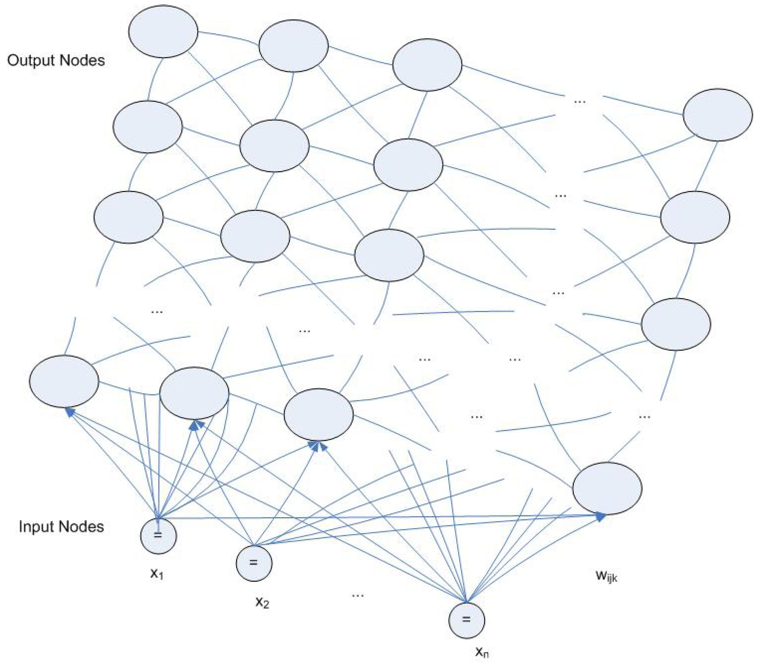
3. ANN Architectures and Training Algorithms

3.1. MLP and BP

Because the original perceptrons, single layer feedfoward networks, which were introduced by Rosenblatt [39], are limited to learning linearly separately patterns, nonlinear layers between the input and output are added to separate the data with enough training to model any well-defined function to arbitrary precision. This MFN model is known as a multilayer perceptron. The neural networks formed using the model are universal approximators [49,50]. Figure 1 shows the diagram of a one-hidden-layered MLP network structure. The MLP networks are typically trained with the BP algorithm. The BP algorithm is supervised, which is to map the process inputs to the desired outputs by minimizing the errors between the desired outputs and the calculated outputs driven from the inputs and network learning.
Figure 1. MLP network structure.
Algorithms 02 00973 g001
The standard BP algorithm [1] is a gradient descent algorithm to minimize the mean square error between the calculated outputs and the desired outputs of the MLP network. Assuming that there are n process inputs, x, and m desired outputs, d, with the network with a sample size of N: {xit, djt | i = 1, 2, … n; j = 1, 2, …, m; t = 1, 2, …, N}, then the mean square error of the network outputs is:
E = 1 2 t = 1 N j = 1 m (d jt y jt ) 2
where yjt is the calculated output.
Based on the gradient descent method, each of the network connection weights is updated as follows:
Δw = η E(w) = η E w = t = 1 l j = 1 m (d jt y jt ) y jt w
where η is a small constant such as 0.1 as the learning rate in the training process of the algorithm. For the MLP in Figure 1, all the weights are the sets of {wik | i = 1, 2, …, n; k = 1, 2, …, h} and {wkj | k= 1, 2, …, h; j = 1, 2, …, m} where h is the number hidden nodes. Each of the output is as follows:
y jt = s( k = 1 h w kj s( i = 1 n w ik x it ))
where s(z) is the activation function of each hidden node and output node. It typically is a sigmoid function as s(z) = 1/(1 + e-z). Therefore,
y jt w kj = s'( k = 1 h w kj s( i = 1 n w ik x it )) [ k = 1 h s( i = 1 n w ik x it )]
y jt w ik = s'( k = 1 h w kj s( i = 1 n w ik x it )) [ k = 1 h s( i = 1 n w ik x it ) + k = 1 h w kj s'( i = 1 n w ik x it )x it ]
and s’(z) = s(z)(1 - s(z)) is the first derivative of s(z).
Earlier than Rumelhart et al. [1], Werbos [44] gave a different derivation of the BP algorithm. This derivation is more general and mathematically rigorous than the one given by Rumelhart et al. In Werbos’ derivation, the chain rule is expressed in a convenient form by ordered derivatives. Even so, most research and applications of the BP algorithm still referred to the results of Rumelhart et al. due to their milestone publication in 1986 with the PDP research group.

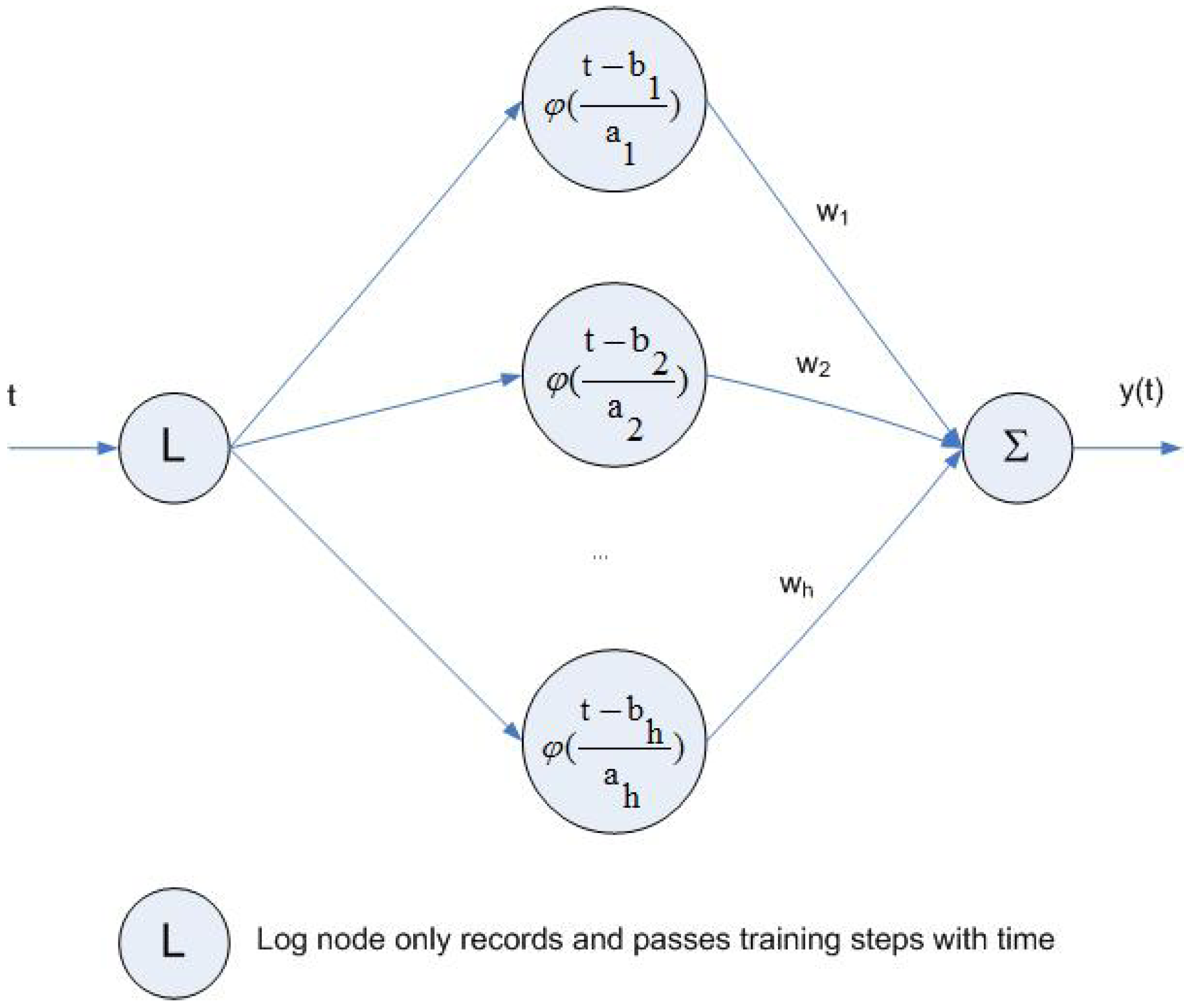
3.2. Radial Basis Function Network

Due to adding hidden nodes and layer(s) and the nonlinearity of the sigmoid activation function of each hidden nodes and/or output nodes in MLPs, the BP algorithm has the possibility to produce complex error surfaces which contain many minima. Since some minima are deeper than others, it is possible that the algorithm will not find a global minima. Instead, the network may fall into local minima, which represent suboptimal solutions. The RBF networks [46] were introduced with the centers of data clustering means, and then the linear solution for the connection weights to the network output directly to a unique local minimum, the global minimum, which shortens network training process greatly.
Figure 2 is a diagram of a one-hidden-layered RBF network structure. The RBF networks also are MFNs. With sufficient larger number of hidden nodes, they are universal approximators as well. The RBF network training also is supervised, involving determination of data clustering centers, ck (k = 1, 2, …, hc), where hc also is the number of the centers to be determined, and network connection weights from the hidden layer to the network outputs, wkj (k = 1, 2, …, hc; j = 1, 2, …, m). Similar to BP training, the RBF training is to establish the map between process inputs and desired outputs by minimizing the errors between the desired outputs and the calculated outputs driven from the inputs and network learning. The objective function of error minimization is defined as:
E = t = 1 N j = 1 m (d jt y jt ) 2
and:
y jt = k = 1 h c w kj R( i = 1 n x it c k )
where R( ) is a RBF function.
A RBF function is any function R that satisfies R(x) = R(||x||). It is a real-valued function that depends on the distance from the origin as R(x) = R(||x||) or from other point or center, c, as R(x - c) = R(||x - c||). The norm ||.|| is usually Euclidean distance.
The linear solution of output layer weights in equation (7) guarantees the objective function (6) to get the global minima and greatly speed up the training process.
RBF networks integrate nonlinear RBF activation functions in hidden layer and linear combination of weights in output layer. In input data clustering, different techniques can be used, such as k-means clustering [60] and fuzzy c-means [61]. There are choices of RBF functions, such as Gaussian RBF, multiquadric RBF, polyharmonic spline, and thin plate spline. Some of the RBFs will bring more parameters to determine in training process, such as Gaussian RBF, R(x - c) = exp(-β||x - c||2), which brings one more parameter, β, to determine.
Figure 2. RBF network structure.
Algorithms 02 00973 g002

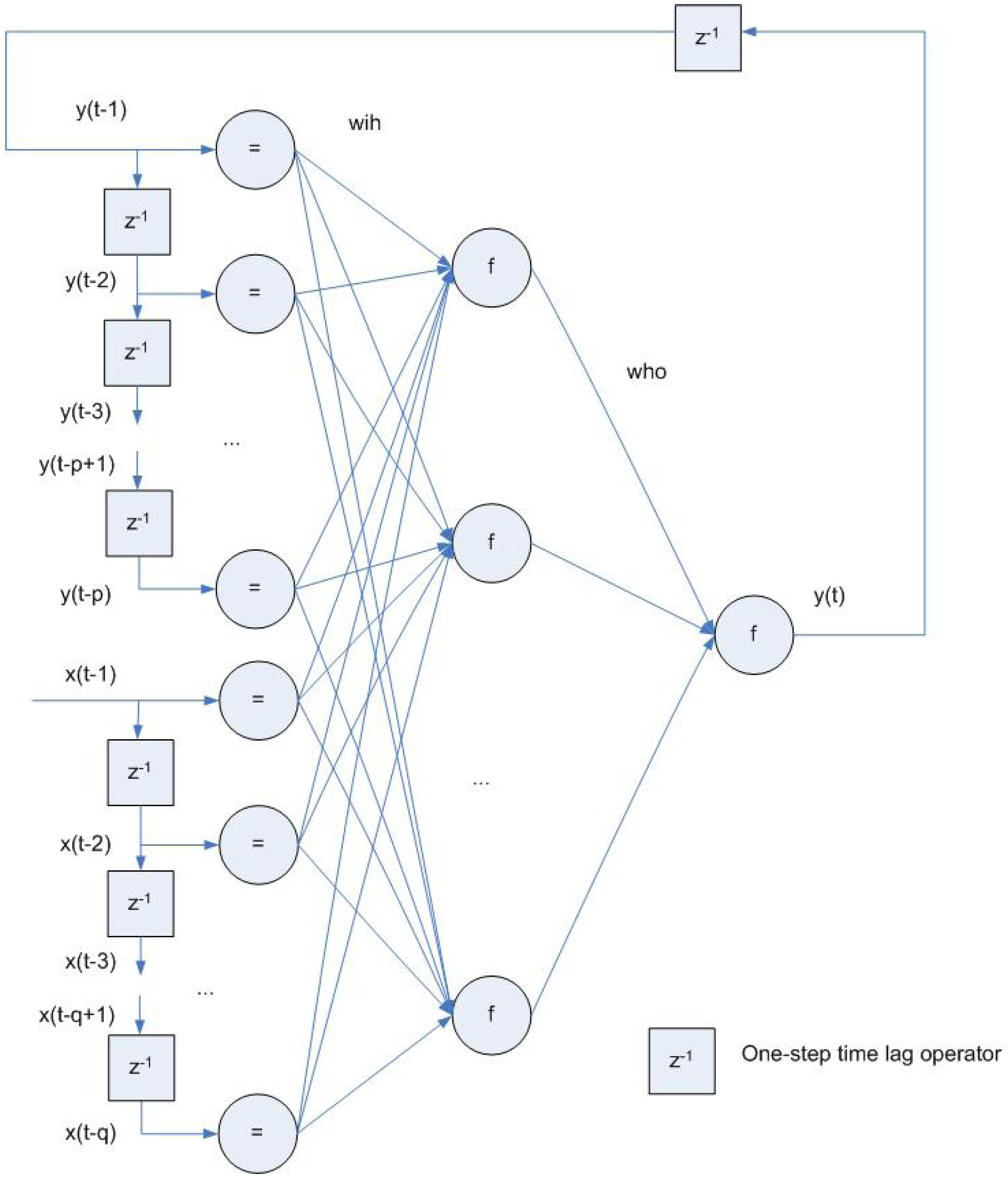
3.3. Recurrent and Feedback Networks

A recurrent neural network is a type of ANN where network nodes may have a directed connection. A typical example of this is that either the network’s hidden node activation values or network output values are fed back into the network input nodes. These types of networks are good at characterizing process temporal dynamics. Examples of simple recurrent networks are Elman and Jordan networks [62,63].
MLP networks are good for mapping the static relationship of process input and output: x → y. They have been used for identification of dynamic systems [64,65]. However, they require a large number of input nodes which may result in long computing time and being affected by external noise [66]. Recurrent neural networks have been attracted in the field of dynamic system identification since they can avoid the problems MLP networks have [67,68,69].
In time series analysis, ANNs can establish AR (AutoRegressive) function map between process input and output: {y(t-i) | i = 1, 2, …, p} → y(t). In process modeling and control, ANNs can help establish ARX (AutoRegressive with eXogenous input) function map of process input and output: {y(t - i), x(t - j) | i = 1, 2, …, p; j = 1, 2, …, q} → y(t) where p and q are the orders of time lags of y and x, respectively. Figure 3 shows a network structure to map the dynamic process input/output relationship with the ARX function map. Internally, this network is identical to a MLP. Externally, it feeds back the network output back to the network input with a lagged time shift. This network is named External Recurrent Neural Network (ERNN) [70]. Obviously, training of this network should be different from standard BP. Around the network, y(t - i) is a time-delayed output from the network itself. This network model is determined as a specific form of time-lag recurrent networks [4]. For the time-lag recurrent networks with only one recurrent connection, i.e. i = 1, a number of training algorithms have been proposed [71,72,73]. Among the proposed algorithms, the BP Through Time (BPTT) is able to be modified for multiple recurrent connections, i.e. i > 1 using ordered derivatives from Werbos’s derivation of the BP algorithm [44]. When the external feedback signal y(t) replaces the input of the network, the change of weights will affect y(t + 1) and thus y(t + 1) all the way to y(N) where T is the length of the data. Thus, the gradient computation has to account for this chaining from t = 0 to t = N. The input layer at time t+1 can be considered as a part of the 3rd layer of the network at time t. When calculating the error of the output layer at time t, it is necessary to calculate the error for the input nodes at time t + 1 up to t + p, all of which are connected to the corresponding output node at time t. In the regular BP algorithm, the error term for the network nodes propagates the required information all the way from t = N back to the current time instant. This is what the BPTT signifies. Based on Werbos’s work [44], a modified BPTT algorithm was derived for the ERNN [74] as described above.
This modified algorithm was used for training over the whole trajectory of the training data. The maximum number of prediction steps is equal to the total number of observations. In controller design, the prediction steps would be much smaller. In order to solve this problem, the network can be trained to do shorter prediction with the modified training algorithm [74]. The modified training algorithm is still BPTT, but at each time instant the error term is propagated from the specified prediction step t + L (L << N) back to the current time instant t. This work resulted in an ERNN-based multiple-step-ahead prediction for process controller design [70]:
y(t + l |t) = f(y(t + l -1|t), ... ,y(t + l -p|t),x(t + l -1), ... ,x(t + l -q),W) y(t + l |t) = { y(t + l  ) when  l > 0 d(t + l  ) otherwise   l = 1,2, ... ,L
where y(t + l |t) is the l-step-ahead predictor of y(t) at the time instant t, f( ) is the approximation of the function map, and W is the set of weights and bias terms in the network.
Figure 3. ERNN network structure.
Algorithms 02 00973 g003

3.4. Kohonen SOM Network and Unsupervised Training

Unlike the trainings of MLP, RBF and ERNN networks, Kohonen SOM networks are trained using an unsupervised algorithm, by which the input data are self-organized into clusters or classes, i.e. similar input data will activate the same network output node. The networks construct one-dimensional, two-dimensional, and even three-dimensional arrays of output nodes to form self-organized feature maps. Figure 4 is the structure of Kohonen SOM network with a two-dimensional array of output nodes used to form feature maps.
This is a two-layer network. The output nodes are orderly arranged in a two-dimensional grid. Each input is connected to all output nodes through a weight. The network training process has two stages. The first is to generate a coarse mapping, i.e. to create some form of topological ordering on the map of randomly oriented nodes. There may be large changes to the orientation of the nodes on the map, so the gain term or adaption rate, η, needs to be kept high to allow large weight modifications and settle into an approximate mapping quickly. Once a stable coarse map is found, the training process goes into the second stage. At this stage, the nodes within the localized regions of the map are fine-tuned to the network inputs. For this fine-tuning much smaller changes of weights must be made at each output node, so the adaptation rate, η, is reduced as training progresses. The weight updating in training is iteratively operated along with winning output node neighborhood:
Δw ijk = η(w ijk -x k ) ij NE ij* (i = 1,2, ... ,p;j = 1,2, ... ,q;k = 1,2, ... ,n)
where p and q the first and second dimension of the feature map array, respectively, n is the number of network inputs, and ij* is the location of optimal output node. The optimal node is determined by:
MIN ij * (D ij ) D ij = k = 1 n (x k w ijk ) 2
Figure 4. Kohonen SOM network with two-dimensional array of output nodes used to form feature maps.
Algorithms 02 00973 g004
The neighborhood function NEij is set large at very beginning of training, and slowly decreases in size with the progress of the training (Figure 5). The output nodes of the network are activated using a winner-take-all method:
y ij = { 1  if  ij = ij* 0  otherwise
That is that if (i,j) is the location of the optimal output node, the output node takes the value of 1; otherwise it takes 0. Accordingly, the weights connected to the neighborhood of the optimal node are updated.
Figure 5. Topological neighborhoods with the progress of training as feature maps are formed.
Algorithms 02 00973 g005

4. Advanced Development of ANNs

With the progress of research and applications, ANN technology has been improved and advanced. Research has been done on modification of the standard BP algorithm to speed up algorithm convergence and avoid local minima in MLP network training. Much work has been devoted to preventing over-fitting in MLPs to improve the generalization ability of the networks. ANNs have been enhanced by fusing with other methods such as fuzzy logic and wavelet analysis. SVMs, emerging as a new soft computing technique, bring up a new wave of research and applications of ANNs.

4.1. Standard BP Enhancement

In standard BP training, it is critical to select a learning rate, η, to let the process converge to the true global minimum of the mean square error of the network outputs with a rather rapid speed. A BP training with a too small learning rate will have a noticeable slow progress. One with a too large learning rate will speed up significantly. However, this may result in oscillations around relatively poor solutions. Evidence shows that the use of a momentum term in the BP algorithm can be helpful in speeding the convergence and avoiding local minima (http://www.cs.bham.ac.uk/~pxt/NC/ASSIGNMENT/MICHAEL/momentum.html). The momentum term is defined as a fraction of the previous weight change αΔw-, and added to equation (2) from the standard BP algorithm [7]:
Δw = η E(w) + αΔw -
where α is taken 0≤ α ≤ 0.9.
In this way, in BP training, the momentum is used to stabilize the weight change using a combination of the gradient decreasing term with a fraction of the previous weight change.
With the concept of momentum in BP training, the method has been further developed. Yu et al. [9] developed an adaptive momentum algorithm which can update the momentum coefficient automatically in every iteration step. The result of this adaptive process is equivalent to adding a momentum term to the standard BP algorithm. The momentum coefficient is updated automatically in every iteration. Numerical simulations show that the adaptive momentum algorithm can eliminate possible divergent oscillations during the initial training, and can also accelerate the learning process and result in a lower error when the final convergence is reached. Gerke and Hoyer [10] presented an analysis of fuzzy adaption of training parameters (learning rate and momentum) to accelerate BP learning in MFNs.
There are other studies on BP training acceleration and local minima. Huang et al. [75] investigated the efficiency of the training processes of MFNs using the gradient descent method in the standard BP algorithm and Levenberg-Marquardt method in backpropagation. It was found that in the case of low epoch training (below several thousand epochs) using the gradient descent algorithm, the Levenberg-Marquardt algorithm was less efficient, and in the case of high epoch training (above several thousand epochs) using the gradient descent algorithm, the Levenberg-Marquardt algorithm was more efficient. Jeenbekov and Sarybaeva [11] described properties of various parameters of sigmoid activation function mathematically with their influence on the speed of convergence of the BP training algorithm for MFNs. Wang et al. [12] proposed an improved BP algorithm intended to avoid the local minima problem caused by neuron saturation in the hidden layer. Each training pattern has its own activation functions of neurons in the hidden layer. When the network outputs have not received their desired signals, the activation functions are adapted so as to prevent neurons in the hidden layer from saturating. Bi et al. [13] proposed a modified error function with two terms. By adding one term to the conventional error function, the modified error function can harmonize the update of weights connected to the hidden layer and those connected to the output layer. Thus, it can avoid thelocal minima problem caused by update disharmony between weights connected to the hidden layer and the output layer. Simulations on some benchmark problems and a real classification task have been performed to test the validity of the modified error function. Otair and Salameh [14] proposed an algorithm used for training that depends on a multilayer neural network with a very small learning rate, especially when using a large training set size. It can be applied in a generic manner for any network size that uses a BP algorithm through an optical time (seen time).

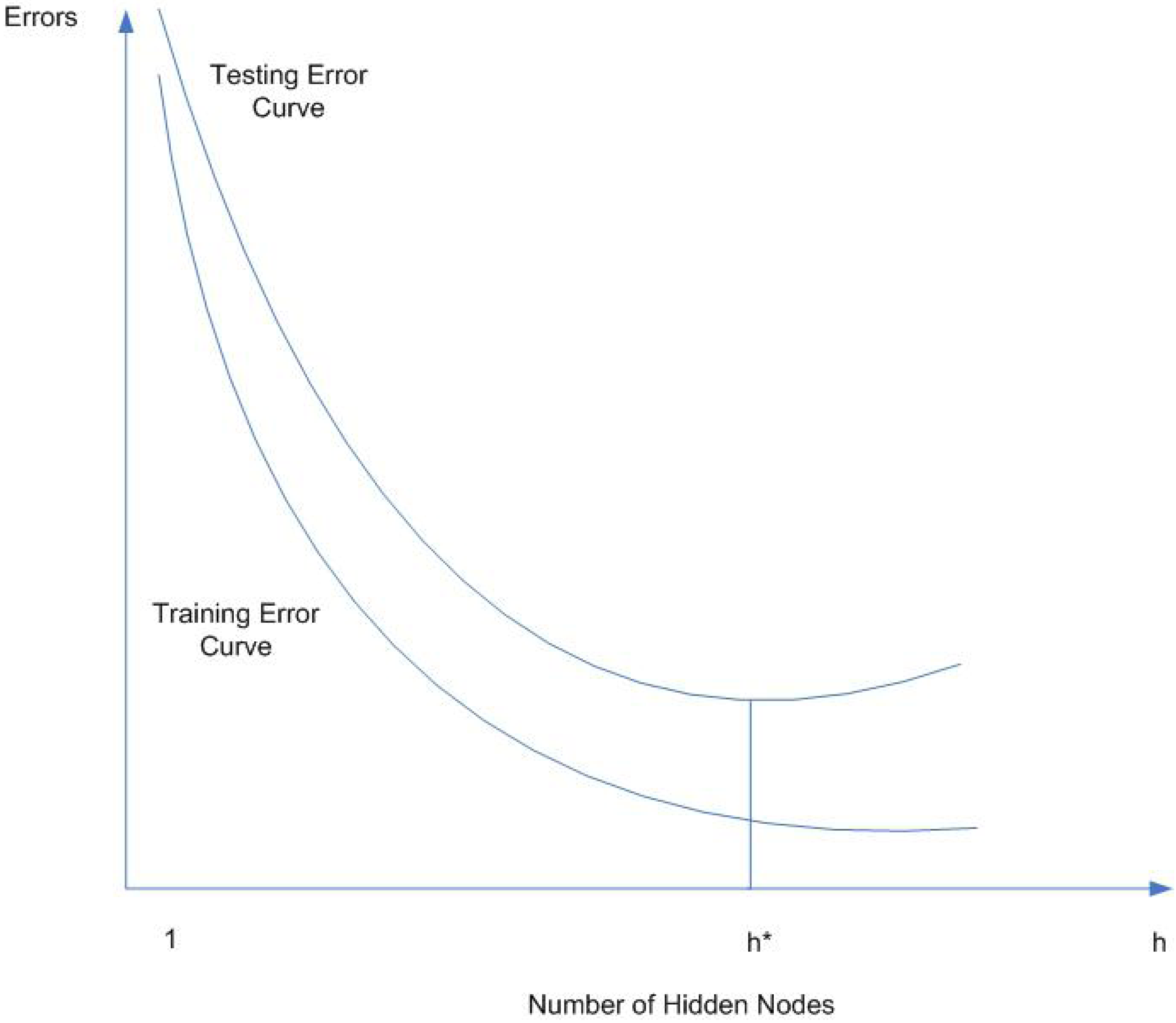
4.2. Network Generalization

Although MFNs can be universal approximators with a sufficiently large number of hidden nodes, excessive number of nodes in the hidden layer may endanger the network to become memorized, which may lead to overfit the input variables [76,77,78]. The overfitted networks may fit training data points well but may not be able to well interpolate and extrapolate testing data points. The testing data points can be between the training points or out of the range of the training points. Overfitting is a very important problem in MLPs, and much work has been devoted to preventing overfitting to improve network generalization with techniques such as early stopping, weight decay, and pruning. Figure 6 shows typical error curves of MLP training and testing. With the increase of the hidden nodes, the training error is large at the beginning and then keeps decreasing with a gradual decline of the curve slope. Similarly, the testing error is also larger at the beginning and then keeps decreasing until it reaches a point, h*. Starting from this point, with further increase of the hidden nodes, the testing error increases gradually while the training error continues to decrease. During training, if the minimal point on the testing curve can be found, the overfitting problem may be solved. The training and testing curves with training steps have a similar behavior as shown in Figure 6, which can be used to investigate overfitting, as can happen with too many training steps.
Based on the explanation of Figure 6, during MLP training, the training error and testing error are checked at every step, and the training process terminates as long as the minimal point of testing error is reached. This is so called early stopping method [20]. Further, a three-set approach was proposed [15]. This approach is to divide a data set into three nonoverlapping subsets: one for training to update network weights, one for testing to terminate training to prevent overfitting, and one for validation to evaluate the trained network. This approach gives a reasonable estimate of the network’s generalization ability.
Adding a penalty term, Ep, to the mean square error of the network outputs in the standard BP algorithm, a new objective function is formulated for MLP training:
Ew = E + λEp
where λ is a pre-set constant for the penalty term. The training algorithm using this objective function causes network weights to converge to smaller absolute values than they would in the standard case. This method is called weight decay [16,75].The generalization ability of a network depends on the adjustment of the decay constant, λ. With weight decay training, the network can avoid oscillation in the outputs caused by large weights.
Figure 6. MLP error curves vs. number of hidden nodes.
Algorithms 02 00973 g006
Network pruning is another method used to prevent overfitting. This method begins with a fully connected network and the network is made smaller by iteratively eliminating least effective nodes in the hidden layer(s) or interconnections between nodes. The pruned network provides a structure that has a greater capacity for generalization [6,18,19].

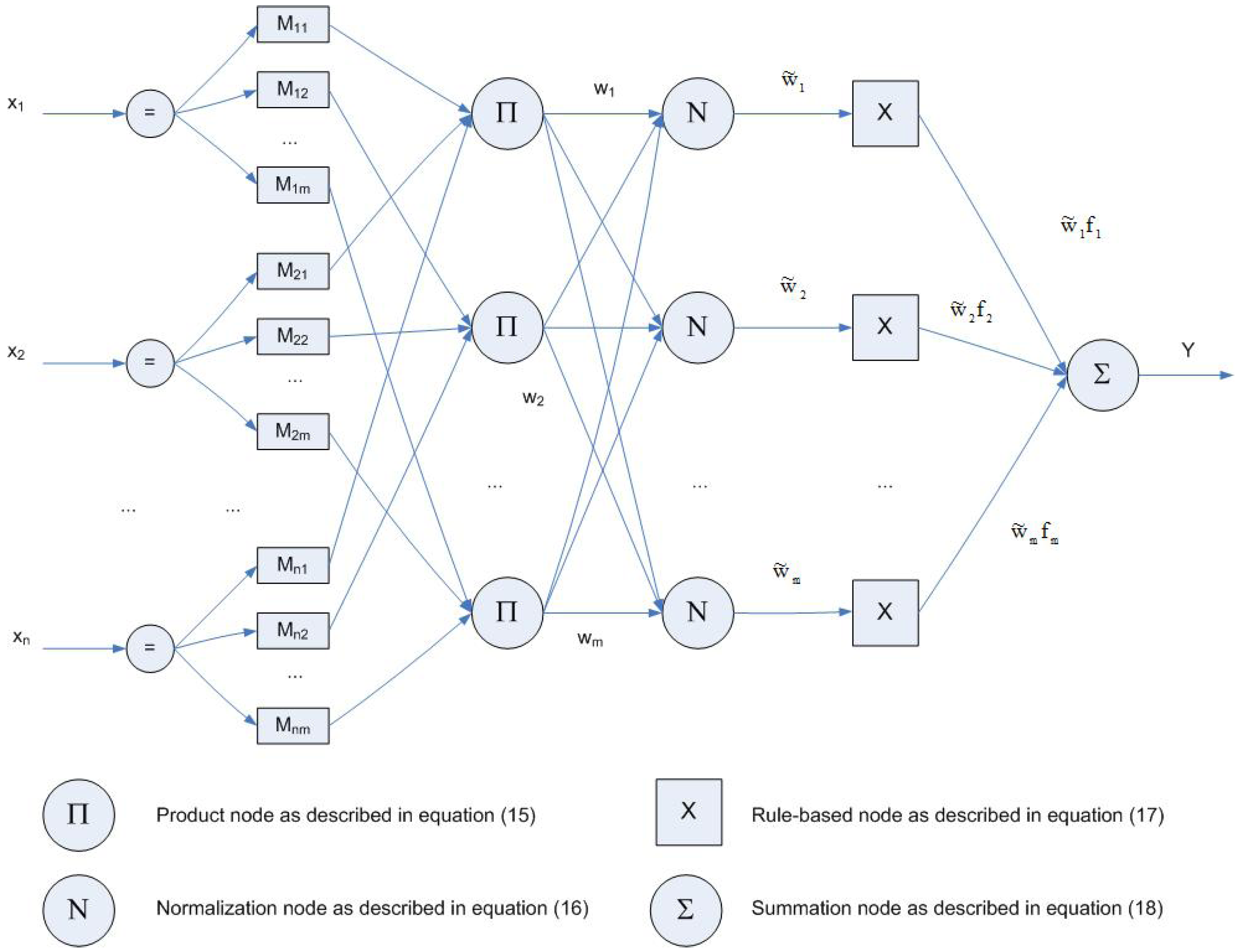
4.3. Neuro-Fuzzy Systems

Fuzzy logic is a form of multi-valued logic derived from fuzzy set theory [79] to deal with reasoning that is approximate, rather than precise. In contrast to yes/no or 0/1 binary logic, Fuzzy logic provides a set of membership values inclusively between 0 and 1 to indicate the degree of truth. Fuzzy logic can be combined with ANNs to form a learning machine that is able to determine the parameters for a fuzzy system by ANN computing. A fuzzy system comprises of linguistic rules such as IF THEN from prior knowledge. Input and output variables of the system are described linguistically. If the knowledge is incomplete, wrong, or contradictory, the fuzzy system needs to be tuned. Fuzzy system is incapable of learning; it is a mechanism of straight interpretation and implementation. ANNs are capable of learning with a sufficient amount of observed examples for a problem. These observations are used to train the network model. The result can provide data for parameterization of fuzzy rules.
The fuzzy-neural systems have been studied and applied. Takagi and Hayashi [22] proposed a neural-fuzzy reasoning system that is capable of automatic determination of inference rules and adjustment according to the time-variant reasoning environment with the use of NN in fuzzy reasoning. Horikawa et al. [23] presented a fuzzy modeling method using fuzzy neural networks with the BP algorithm. The method can identify the fuzzy model of a nonlinear system automatically. Nie and Linkens [24] approximated reasoning through a BP Neural Network with the aid of fuzzy set theory. An example of multivariable fuzzy control of blood pressure was examined for the underlying principles. Simpson and Jahns [25] introduced the fuzzy min-max function approximation neural network. The function approximation network is realized by modifying the developed fuzzy min-max clustering network [80] to include an output layer that sums and thresholds the hidden layer membership functions. Jang [81] introduced the framework of ANFIS (Adaptive-Network-based Fuzzy Inference System). Jang and Sun [27] reviewed fundamental and advanced developments in neuro-fuzzy systems for modeling and control. They introduced design methods for ANFIS in modeling and control applications.
A fuzzy-neural system can be represented as a MFN. The first layer is for input variables. The middle or hidden layer(s) are for encoding fuzzy rules and fuzzy inference. The last layer is for output variables. The fuzzy inferences are converted as network connection weights. Figure 7 shows the structure of a fuzzy-neural system based on the idea of ANFIS [81].
Figure 7. Structure of a fuzzy-neural system.
Algorithms 02 00973 g007
For n input variables {xi | i = 1, 2, …, n}, suppose that there are m fuzzy if-then rules:
Rule 1: If x1 is M11, x2 is M21, …, and xn is Mn1, then f1=a11x1+a12x2+…+a1nxn+r1
Rule 2: If x1 is M12, x2 is M22, …, and xn is Mn2, then f2=a21x1+a22x2+…+a2nxn+r2
… … …
Rule m: If x1 is M1m, x2 is M2m, …, and xn is Mnm, then fm=am1x1+am2x2+…+amnxn+rm
where Mij is a linguistic label (small, medium, and large) of a membership function, μMij(x), of xi with the associated node j. The membership function can be in different forms with different parameter sets, such as the generalized bell-shaped function,
μ M ij (x) = 1 1 + [( x c ij a ij ) 2 ] b ij
or the Gaussian function, μ M ij (x) = exp[ ( x b ij a ij ) 2 ] . In the layer, each node labeled Π multiplies the incoming membership values and sends the product out to the next layer as connection weights:
w j = μ M 1j (x) × μ M 2j (x) × ... × μ M nj (x)       ( =  1 ,  2 ,   ,  m )
In the next layer labeled N, the connection weights are normalized:
w ˜ j = w j i = 1 m w i       ( =  1 ,  2 ,   ,  m )
In the next layer the outputs are:
y j = w ˜ j f j = w ˜ j (a j1 x 1 + a j2 x 2 + ... + a jn x n + r j )       ( =  1 ,  2 ,   ,  m )
In the last node, the node generates the overall output of the network by summing up from all incoming connections:
Y = i = 1 m y i = i = 1 m w ˜ j f i = i = 1 m w i f i i = 1 m w i
The parameters included in the fuzzy and neural network equations above can be updated using the method of gradient descent in the standard BP algorithm. Other methods were suggested also to update the parameters [81].

4.4. Wavelet-Based Neural Networks
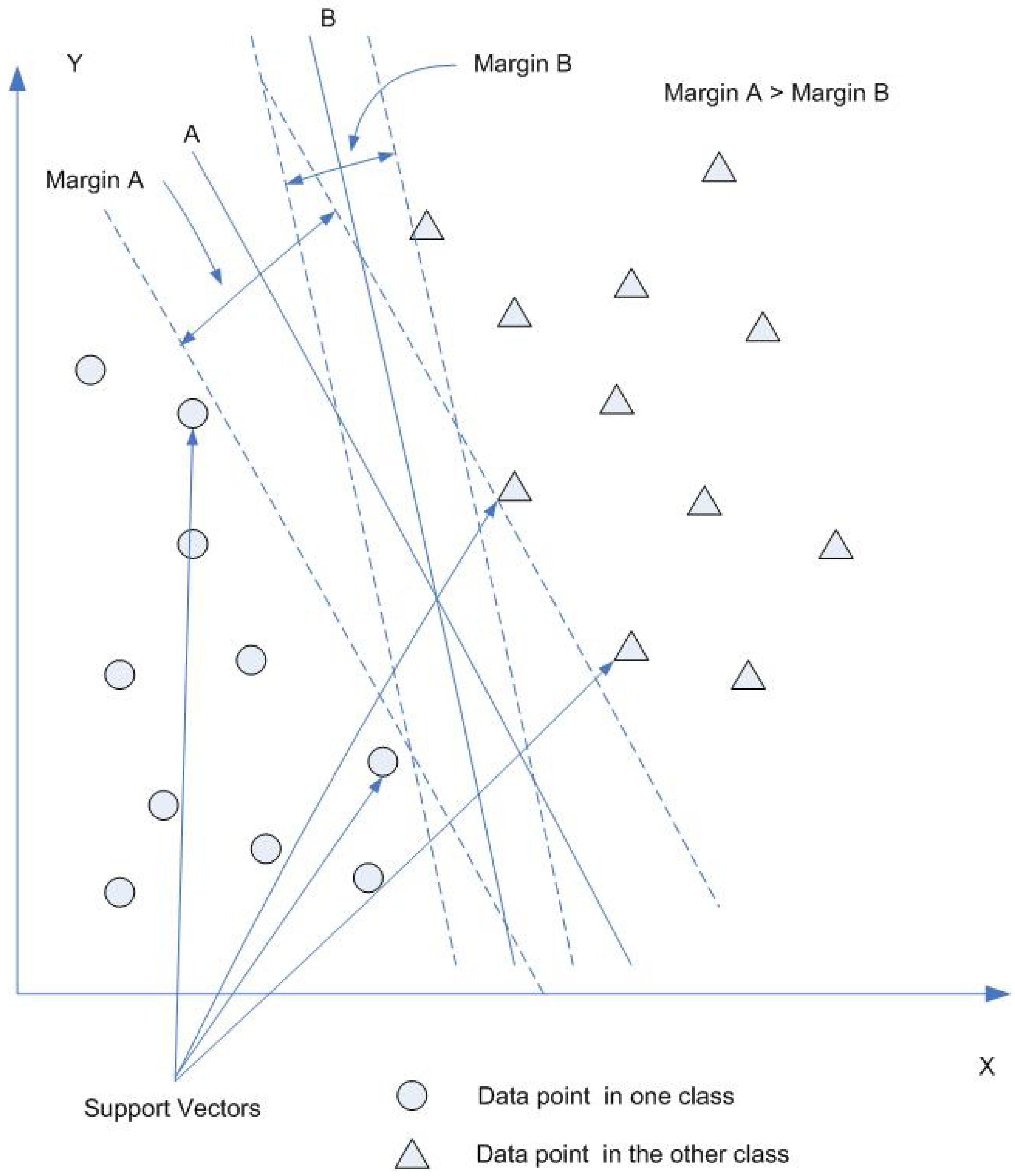
As discussed above, the standard BP algorithm may produce problems in training, for example, converge to local optima. Besides, the determination of the network structure in BP training, such as the number of hidden nodes, is still subjective. With the intelligent integration of wavelet transform, ANNs can be able to approximate data with non-linear and non-stationary properties and to conduct self-learning adaptive structure identification and parameter estimation in modeling process.
Wavelets are “small’’ waves that should integrate to zero around the x-axis. They localize functions well and a “mother’’ wavelet can be translated and dilated into a series of wavelet basis functions. The basic idea of wavelets can be traced back to very early in this century. However, the development of the construction of compactly supported orthonormal wavelets [82] and the wavelet-based multiresolution analysis [83] has resulted in extensive research and applications of wavelets in recent years. In comparison to the more widely known Fourier transform, wavelet basis functions are local both in frequency and time while Fourier basis functions are local only in frequency. Wavelet analysis has been widely used in a variety of fields, especially in signal and image processing.
Wavelet analysis is becoming a common tool for analyzing localized variations of power within a time series [84]. By decomposing a time series into time-frequency space, one is able to determine both the dominant modes of variability and how those modes vary in time. Wavelet-based ANNs (WANNs) have been developed and used for function approximation [28,29,30]. WANNs have been further developed for nonlinear time series forecasting [31]. WANNs have a strong ability of function approximation for optimal time series pattern recognition and their modeling algorithms are different from conventional BP neural network training algorithms. Therefore, WANNs have the potential to overcome the problems that conventional ANNs had.
WANN is a MFN model with wavelet analysis. It replaces the sigmoid function in the MLP with nonlinear wavelet basis function, ϕ ( t b a ) , where a and b are the scale factor and translation factor of the wavelet function, respectively. In this model, nonlinear time series is expressed as a linear combination of selected nonlinear wavelet basis so that a finite number of wavelet series items are used to approximate time series function, i.e.
y(t) = i = 1 h w i ϕ ( t b i a i )
Figure 8 shows the structure of the WANN. This is a single hidden-layered feedforward network. It only has one input node and one output node. The objective of the modeling task is to determine the network parameters, wi, ai, bi and h, to achieve an optimal fitting between the desired output series d(t) and the calculated output series y(t):
J h = 1 2 t = 1 N [d(t)-y(t)] 2
Figure 8. Structure of WANN.
Algorithms 02 00973 g008
Unlike in the standard BP algorithm, in WANN training determination of h is a step-wise process. Preset a toleranceε for nonlinear time series fitting error. Starting h from 1 and calculate J1. If J1 < ε, the optimal h, h* = 1; otherwise, set h = 2 and calculate J2. If J2<ε, h* = 2; otherwise, keep on going until h* is found with Jh* < ε.
Using Newton’s method it can be derived that the parameter updating equations can be as follows in training:
Δ w i = t = 1 N [d(t)-y(t)] ϕ ( t-b i a i )
Δ a i = t = 1 N [d(t)-y(t)] w i a i 2 ( t b i ) ϕ ' ( t-b i a i )
Δ b i = t = 1 N [d(t)-y(t)] w i a i ϕ ' ( t-b i a i )
The forms of ϕ (t) and ϕ ' (t) depend on the selected wavelet function. For example, for Morlet mother wavelet, φ(t) = cos(1.75t)exp(–t2/2). Then its first derivative is φ′(t) = –1.75sin(1.75t)exp(–t2/2) –tcons(1.75t)exp(–t2/2).

4.5. SVMs

SVMs were proposed by Vapnik [85]. Based on the description of Burges [32] and Cristianini and Taylor [33], SVMs are a set of supervised generalized linear classifiers that have often been found to provide higher classification accuracies than widely used MLP classifiers. The growing interest in SVMs is shown by their successful application in many areas such as automobile [86], time series analysis [87,88], medicine [89], pattern recognition [90], geophysics [91,92], computational biology [93], and control engineering [94]. The interest resulted from SVMs’ intrinsic effectiveness with respect to traditional classifiers. This effectiveness results in high classification accuracies and very good generalization capabilities. In architecture design, SVMs requires limited effort to configure few control parameters compared with traditional classifiers such as MLPs. Also, based on the universal approximation capability of their standard MFN counterparts, the approximation capability of SVMs was investigated [51]. It was shown that an SVM with polynomial kernel of degree n-1, which is trained on a training set of size n can approximate the n training points up to any accuracy.
A SVM performs classification through mapping input vectors into a higher-dimensional space and constructing a hyperplane that optimally separates the data in the higher-dimensional space. A SVM model using sigmoid kernel function is equivalent to a two-layer perceptron neural network. However, the operation of the SVM is different. In training, a SVM implements a simple linear mapping or linear classifier together with a prior fixed nonlinear mapping in order to make data separable. This implementation allows training to not suffer from the problem of local minima, and to focus on function optimization with respect to its generalization ability. These advantages often lead to better results for SVMs compared to MFNs.
The goal of SVM modeling is to find the optimal hyperplane that separates clusters of vectors, a set of features, such that data points with one class of the variable are on one side of the plane and ones with the other class are on the other side of the plane. The vectors near the hyperplane are the support vectors. Let’s look at the 2-dimensional case as an example. Assume that for classification, the data are from a categorical variable with two classes, and there are two prediction variables, X and Y, with continuous values. The data points using the value of X on the X axis and Y on the Y axis may be plotted as Figure 9.
Figure 9. Margin between support vectors in two-dimension.
Algorithms 02 00973 g009
In the plot it can be seen what classes each (X,Y) point belongs to. In this example, the data points with one class are in the lower left corner of the plot and the data points with the other classes are in the upper right corner. The SVM analysis is find a one-dimensional hyperplane, i.e. a line, to separate the data points based on their target classes. Obviously, there are an infinite number of possible such lines. Two of them are shown in the plot. The task of SVM now is to determine which line is optimal. For this optimization two parallel (dashed) lines are constructed, one on each side of the separating line. The two lines are pushed up against the two sets of data points belonged to two classes. They label the distance between the separating line and the closest vectors to the line. The two lines are used to calculate the margin, which is defined as the distance between them. The SVM analysis is to find the line (hyperplane in general) that makes the margin between the support vectors maximized. In Figure 9, the line A is superior to the line B. In this sense, SVM classifiers are also known as maximum margin classifiers.
Mathematically, suppose having a training data pairs {(xi, ci) | i= 1, 2, …, N} with xi ∈ Rn and ci∈{1, -1}, indicate what class the data point xi belongs to. In a simple case, a hyperplane can be defined as F(x) = wtx + w0 where w is the adaptable weight vector and w0 is the bias term, and T is the vector transpose operator. In training, the data points xi are projected into the higher-dimensional space, and the classification is conducted through sign[f(x)] where f(x) is the estimate of F(x). The SVM algorithm searches for a hyperplane f(x) that maximizes the margin between the two sets of data points in class 1 and -1.
Further, the margin maximum problem can be solved in any high-dimensional space by introducing a kernel function [95,96]. With a nonlinear kernel function, the low-dimensional input space is nonlinearly transformed into a high-dimensional feature space such that the probability that the feature space is linear separable becomes higher. Theoretically, the kernel function is able to implicitly map the input space into an arbitrary high-dimensional feature space that can be linearly separable even if the input space may not be linearly separable. Some commonly used kernel functions are polynomial, Gaussian, Sigmoid, and RBF.
In general, SVMs’s training is to solve the following optimization problem:
MIN w, w 0 ( 1 2 w T w + λ i = 1 N ξ i )
s.t.   c i [w T φ (x i ) + w 0 ] 1 ξ i
where λ is a user defined positive constant, a penalty parameter of the error term, ξi (≥0) is the slack variable to measure the degree of misclassification of xi, and φ(x) is the function to map data points xi from the input space to a higher-dimensional feature space.
With equation (22), data points xi are mapped into a higher-dimensional space by the function of φ(x). Then a linearly separable hyperplane ( w T φ (x i ) + w 0 ) is found with the maximal margin in the higher-dimensional space. Further, the mapping function φ(x) is determined with a specified kernel function K(xi,xj):
K(xi,xj) = φ(xi) φ(xj)
If RBF is chosen as the kernel function, then K(xi, xj) = exp(-γ||xi - xj||2) (γ > 0). The RBF kernel is good at handling nonlinear classification for SVMs.

5. Limitations of ANNs

As described above, ANNs are powerful computing techniques, which are designed to mimic human learning processes by establishing linkages between process input and output data. These techniques have been widely applied with advanced development with their unique advantages, such as no underlying assumption about the distribution of data, arbitrary decision boundary capabilities, universal approximation capabilities, easy adaptation to different types and structures of data, ability to fuzzy output values to enhance classification, and good generalization capabilities. However, ANNs have some disadvantages in common, which need to be considered in practical application:
  • Black box
    ANNs are black box in nature. Therefore, if the problem is to find the output response to the input such as system identification [96], ANNs can be a good fit. However, if the problem is to specifically identify causal relationship between input and output, ANNs have only limited ability to do it compared with conventional statistical methods.
  • Long computing time
    ANN training needs to iteratively determine network structure and update connection weights. This is a time-consuming process. With a typical personal computer or work station, the BP algorithm will take a lot of memory and may take hours, days and even longer before the network converges to the optimal point with minimum mean square error. Conventional statistical regression with the same set of data, on the contrary, may generate results in seconds using the same computer.
  • Overfitting
    With too much training time, too many hidden nodes, or too large training data set, the network will overfit the data and have a poor generalization, i.e. high accuracy for training data set but poor interpolation of testing data. This is an important issue being investigated in ANN research and applications as described above.
Also, SVMs were originally developed to solve binary classification problems. How to effectively extend it for multiclass classification is still an ongoing research issue. Typically, a multiple class classifier can be constructed by combining several binary classifiers. Further, all classes can be considered at once. Hsu and Lin [98] gave decomposition implementations for two such "all-together" methods. They compared the performance with three methods based on binary classifications: one-against-all, one-against-one, and Directed Acyclic Graph SVM (DAGSVM). The experiments indicated that the one-against-one and DAG methods are more suitable for practical use than the other methods.

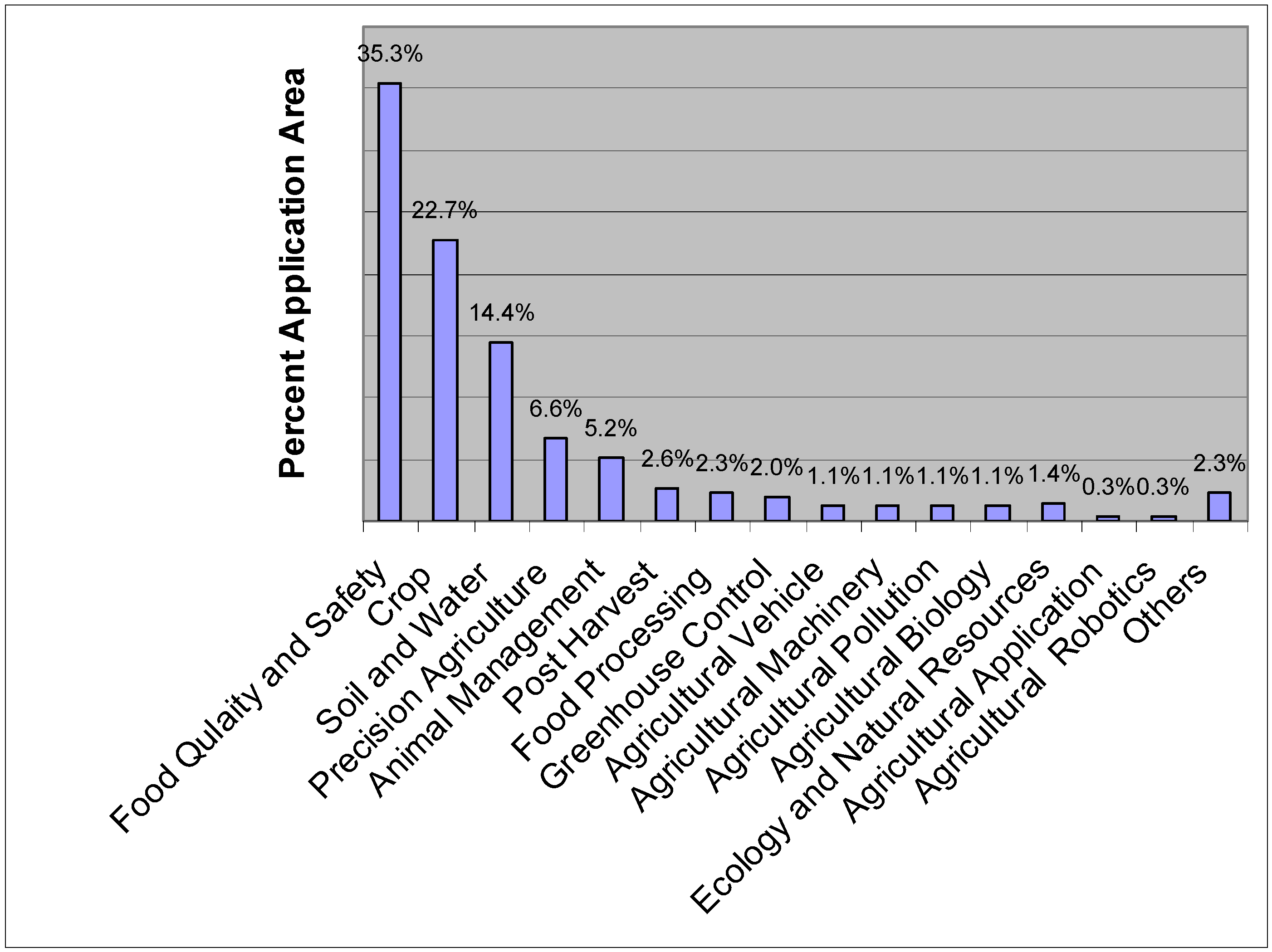
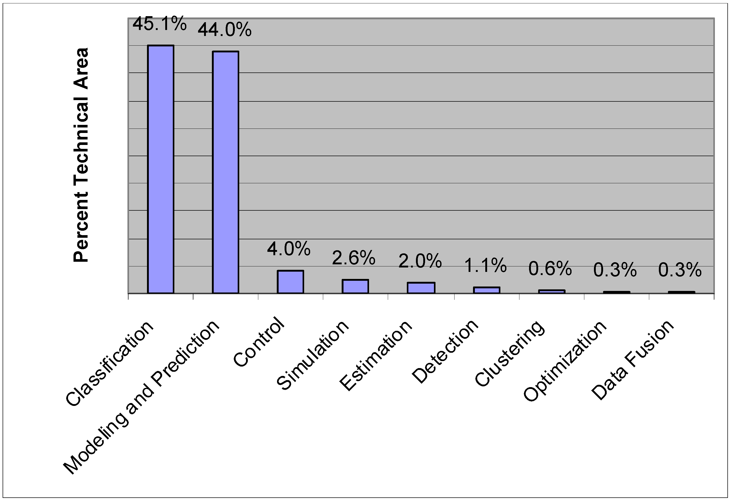
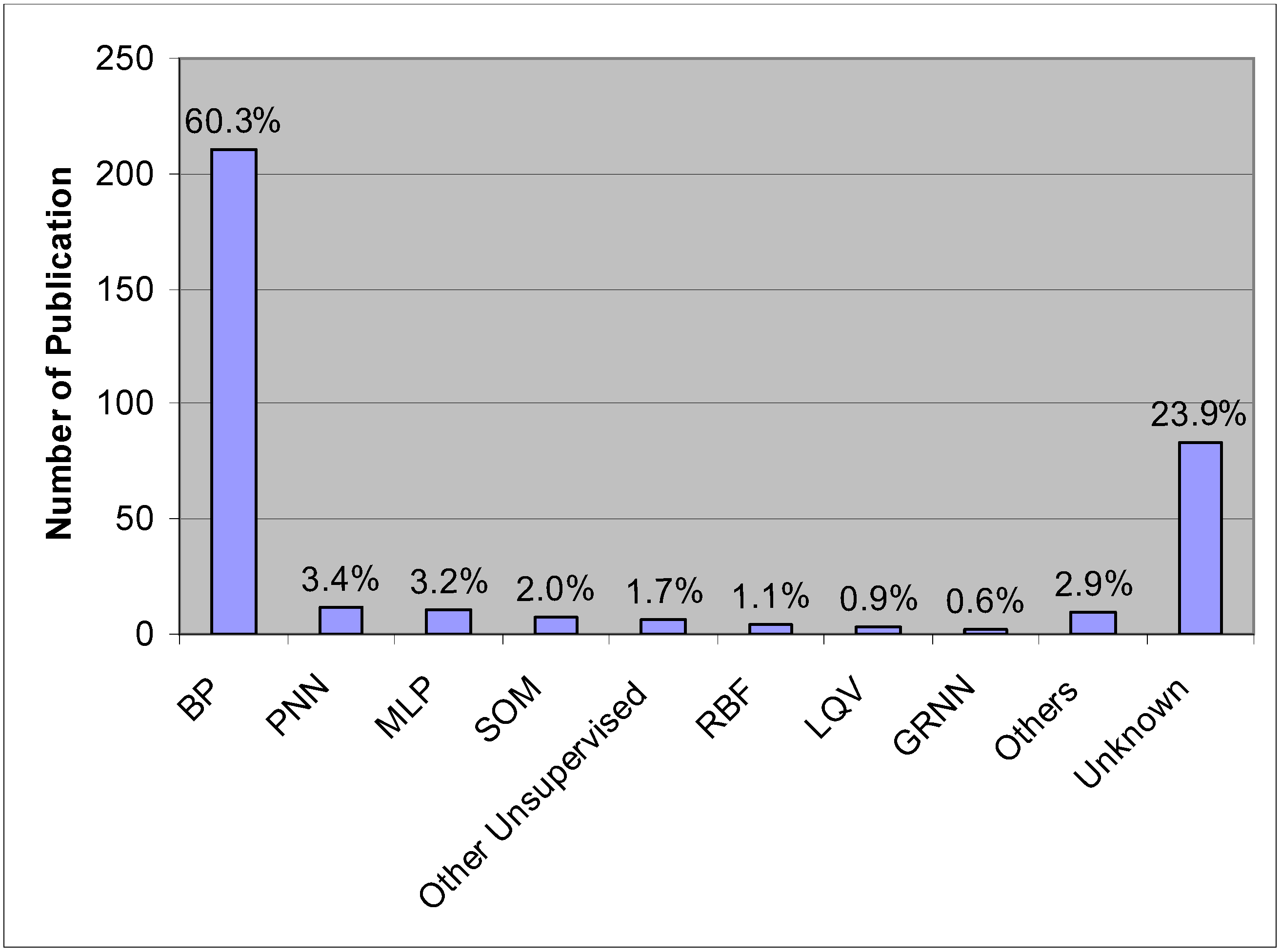
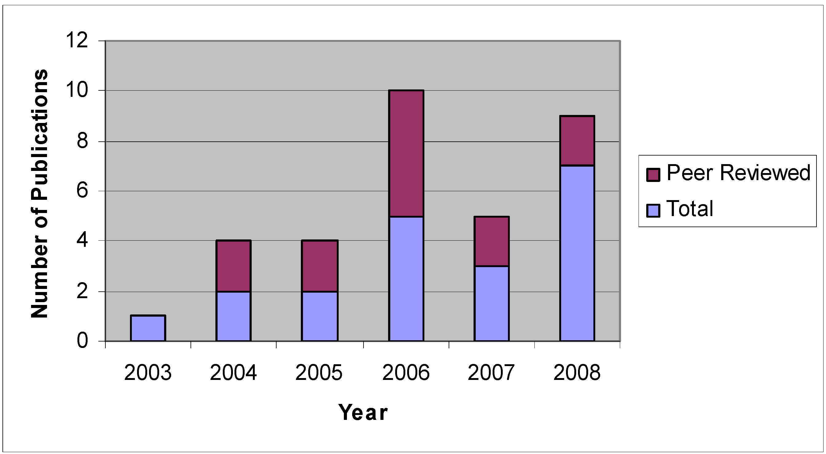
6. ANN Applications in Agricultural and Biological Engineering

ANNs have the largest body of applications in agricultural and biological engineering compared to other soft computing techniques such as fuzzy logic and genetic algorithms. In summary of related 348 papers and reports, ANNs have been applied in solving problems in food quality and safety (35.3%), crop (22.7%), soil and water (14.4%), precision agriculture (6.6%), animal management (5.2%), post harvest (2.6%), food processing (2.3%), greenhouse control (2%), agricultural vehicle control (1.2%), agricultural machinery (1.2%), agricultural pollution (1.2%), agricultural biology (1.2%), ecology and natural resources (1.4%), agricultural robotics (0.3%), chemical application (0.3%), and others (2.3%) such as bioenergy and agricultural facilities (Figure 10). These ANN applications have been created mainly through classification (45.1%), modeling and prediction (44%), control (4%), and simulation (2.6%), parameter estimation (2%), detection (1.2%), data clustering (0.6%), optimization (0.3%) and data fusion (0.3%) as well (Figure 11).
Early applications include modeling sensory color quality of tomato and peach [99], investigation of combined effects of CO2 and sucrose on the growth of alfalfa cuttings using a Kalman filter neural network [100], classification of apple surface features [101], corn kernel breakage classification [102], and machine vision inspection of potatoes [103].
Recently, the BP ANN method was used in regression for modeling the correlation between crop yield and 10 yield components of chickpea [104]. A BP ANN was employed and trained with extracted features from the data collected by electronic nose to identify the wheat age [105]. BP neural network and generalized regression neural network techniques were developed and compared to model source gas and PM10 concentration and emission rate (GPCER) generated and emitted from swine deep-pit finishing buildings as affected by time of day, season, ventilation rates, animal growth cycles, in-house manure storage levels, and weather conditions [106]. MLP models were developed and used to predict or classify water stress in samples of Sunagoke moss using the texture features extracted from color co-occurrence matrix (CCM) and gray-level co-occurrence matrix (GLCM) methods [107]. A BP ANN was developed for predicting fungal infections using input from principal components extracted from sample visible and near-infrared (NIR) reflectance spectroscopy for early detection of Botrytis cinerea on eggplant leaves [108].
Figure 10. Application area distribution of ANNs in agricultural and biological engineering.
Algorithms 02 00973 g010
Figure 11. Technical area distribution of ANNs in agricultural and biological engineering.
Algorithms 02 00973 g011
Similar to applications in general engineering fields, most of the work in agricultural and biological engineering has been accomplished by multilayer feedforward ANN trained by the famous BP algorithm, which was inspired by the work of Rumelhart et al. in 1986. Among the 348 collected papers and reports, besides 83 of them in which the ANNs’ structure and training algorithm were not explicitly stated, 210 of them (60%) were based on MFNs trained by the BP algorithm. Twelve of them (3.5%) were based on PNN (Probabilistic Neural Network). Eleven of them (3%) were based on MLP using different training algorithms such as Levenberg-Marquardt optimization procedure, Broyden-Fletcher-Goldfarb-Shanno (BFGS) optimization procedure, and genetic algorithm. Seven of them (2%) were based on Kohonen SOM. Six of them (2%) were based upon other unsupervised training algorithms such as fuzzy art, ART2 and Auto- Associative network. Four of them (1%) were based on RBF networks. Three of them (0.8%) were based on LVQ (Learning Vector Quantization). Two of them (0.6%) were based on GRNN (Generalized Regression Neural Network). Ten of them (3%) were based on other network structures such as Counter-Propagation (CP) and Adaptive Logic Network (ALN). Figure 12 shows the ANN method distribution of applications in agricultural and biological engineering.
Fuzzy-neural systems have been developed and used in agricultural and biological engineering. Table 1 listed papers and reports on fuzzy-neural methods and systems in applications in agricultural and biological engineering. Linko et al. [109] applied neural network modeling for fuzzy food extrusion control. Kim and Cho [110] used the BP algorithm in training ANN models for prediction of volume, browning and bread temperatures. The outputs of the ANN models were used for fuzzy control simulation of the oven used in the baking process. Morimoto et al. [111] proposed and then applied a new fuzzy control technique, which efficiently selects optimal membership functions and control rules by using neural networks and genetic algorithms to the control of relative humidity in a fruit-storage house. The response of relative humidity, as affected by ventilation, was first identified using neural networks, and then optimal membership functions and control rules were sought through simulation of the identified model using GAs. Odhiambo et al. [112] developed a strategy consisting of fusing the fuzzy logic and ANN on a conceptual and structural basis for an easy and efficient means of tuning fuzzy ET (Evapotranspiration) models. The neural component provided supervised learning capabilities for optimizing the membership functions and extracting fuzzy rules from a set of input–output examples selected to cover the data hyperspace of the sites evaluated.
Figure 12. ANN method distribution of applications in agricultural and biological engineering.
Algorithms 02 00973 g012
Table 1. Papers and reports on fusion of fuzzy logic and ANNs in agricultural and biological engineering.
YearAuthorFusion TypeApplication Area
1992Linko et al. [109]ANN modeling for fuzzy controlExtrusion control
1997Kim and Cho [110]ANN modeling plus fuzzy control simulationBread baking process control
1997Morimoto et al. [111]ANN modeling plus GA parameter optimization for fuzzy controlFruit storage control
2001Odhiambo et al. [112]Conceptual and structural fusion of fuzzy logic and ANNET model optimization
2003Andriyas et al. [118]FCM clustering for RBF trainingPrediction of the performance of vegetative filter strips
2003Chtioui et al. [113]SOM with FCM clusteringColor image segmentation of edible beans
2003Lee et al. [119]ANFIS modelingPrediction of multiple soil properties
2003Neto et al. [120]ANFIS classificationAdaptive image segmentation for weed detection
2004Odhiambo et al. [115]Fuzzy-Neural Netwok unsupervised classificationClassification of soils
2004Meyer et al. [114]ANFIS classificationClassification of uniform plant, soil, and residue color images
2004Goel et al. [121]Fuzzy c-means clustering for RBF trainingPrediction of sediment and phosphorous movement through vegetative filter strips
2006Hancock and Zhang [115]ANFIS classificationHydraulic vane pump health classification
2007Xiang and Tian [117]ANN modeling plus ANFIS training of fuzzy logic controllerOutdoor automatic camera parameter control
Chtioui et al. [113] developed a novel segmentation approach that partitions color images into two uniform regions is described. This unsupervised procedure is based on a SOM neural network and fuzzy c–means clustering (FCM). The SOM allows the mapping of a color image related to edible beans into a consistent two–dimensional table through a non–linear projection. Fuzzy clustering is then applied to the Kohonen map to determine the two cluster centers. Meyer et al. [114] conducted a digital camera operation study for classifying uniform images of grass, bare soil, corn stalks residue, wheat straw residue, and a barium sulfate reference panel, based on color. The classifications were conducted with fuzzy inference systems, built with subtractive clustering, an ANFIS. Odhiambo et al. [115] applied a fuzzy-neural network (F-NN) classifier for unsupervised clustering and classification of soil profiles using ground-penetrating radar (GPR) imagery. Hancock and Zhang [116] developed an on-line hydraulic vane pump fault detection system. This fault detection system decomposed vertical pump vibration signals using wavelet packet analysis. Packets containing signal features distinguishing normal and failed pump operation were entered into an ANFIS for pump health classification. Xiang and Tian [117] developed an artificially intelligent controller based on an ANN and an ANFIS for implementing controller to automatically adjust multispectral camera parameter to compensate for changing natural lighting conditions and to acquire white-balanced images.
The interest of SVMs in agricultural and biological engineering is steadily growing (Figure 13). The figure indicates that although the number of peer reviewed publications on this topic did not increase steadily over the past few years, a trend exists for total number of papers and report to increase in the past few years and to be able to project this trend in the next few years. The successful implementations of SVMs in agricultural and biological engineering are listed in Table 2, which includes classification of intact and cracked eggs [122], classification of forest data cover types [123], classification of meat with small data set [124], black walnut shell and meat classification using hyperspectral fluorescence imaging [125], classification to differentiate individual fungal infected and healthy wheat kernels [126], classification for weed and nitrogen stress detection in corn [127], discrimination for screening of compound feeds using NIR hyperspectral data [128], identification of tea varieties by computer vision [129], discrimination of wheat classes with NIR spectroscopy [130], detection of underdeveloped hazenuts from fully developed nuts by impact acoustics [131], classification of electronic nose data [132], classification of modified starches [133], classification of milk with an electronic nose [134], and recognition of plant disease [135]. In these applications, Zhang et al. [126] fused SVM with kernel of RBF neural network. Pardo and Sberveglieri [132] implemented SVM with RBF kernel. Brudzewski et al. [134] applied SVM neural network with one hidden layer of non-linear neurons, one-output linear neuron and specialized learning procedure leading to the global minimum of the error function and excellent generalization ability of the trained network.
Figure 13. Publications on applications of SVMs in agricultural and biological engineering.
Algorithms 02 00973 g013
Table 2. Papers and reports on applications of SVMs in agricultural and biological engineering.
YearAuthorApplication MethodApplication Area
2003Fletcher and Kong [136]SVM classificationClassifying feature vectors and decide whether each pixel in hyperspectral fluorescence images of poultry carcasses falls in normal or skin tumor categories
2004Brudzewski et al. [134]SVM neural network classificationClassification of milk by an electronic nose
2004Tian et al. [135]SVM classificationClassification for recognition of plant disease
2005Pardo and Sberveglieri [132]SVM with RBF kernel of RBFClassification of electronic nose data
2005Pierna et al. [133]SVM classificationClassification of modified starches by Fourier transform infrared spectroscopy
2006Chen et al. [129]SVM classificationIdentification of tea varieties by computer vision
2006Karimi et al. [127]SVM classificationClassification for weed and nitrogen stress detection in corn
2006Onaran et al. [131]SVM classificationDetection of underdeveloped hazenuts from fully developed nuts by impact acoustics
2006Pierna et al. [128]SVM classificationDiscrimination of screening of compound feeds using NIR hyperspectral data
2006Wang and Paliwal [130]Least-Squares SVM classificationDiscrimination of wheat classes with NIR spectroscopy
2007Jiang et al. [125]Gaussian kernel based SVM classificationBlack walnut shell and meat classification using hyperspectral fluorescence imaging
2007Oommen et al. [137]SVM modeling and predictionSimulation of daily, weekly, and monthly runoff and sediment yield fron a watershed
2007Zhang et al. [126]Multi-class SVM with kernel of RBF neural networkClassification to differentiate individual fungal infected and healthy wheat kernels.
2008Fu et al. [138]Least-Squares SVM modeling and predictionQuantification of vitamin C content in kiwifruit using NIR spectroscopy
2008Khot et al. [124]SVM classificationClassification of meat with small data set
2008Kovacs et al. [139]SVM modeling and predictionPrediction of different concentration classes of instant coffee with electronic tongue measurements
2008Peng and Wang [140]Least-Squares SVM modeling and predictionPrediction of pork meat total viable bacteria count with hyperspectral imaging
2008Sun et al. [106]SVM modeling and predictionOn-line assessing internal quality of pears using visible/NIR transmission
2008Trebar and Steele [123]SVM classificationClassification of forest data cover types
2008Yu et al. [9]Least-Squares SVM modeling and predictionRice wine composition prediction by visible/NIR spectroscopy
2009Deng et al. [122]SVM classificationclassification of intact and cracked eggs

7. Conclusion and Future Directions

As described above, ANNs have their advantages and have been used as a powerful tool in solving problems in scientific research and engineering applications. ANNs have their own limitations to restrict them as a substitute of traditional methods such as statistical regression, pattern recognition, and time series analysis. In the next decade with advanced development of computer power, ANNs will continue to develop new applications in various fields, including agricultural and biological engineering. As a powerful alternative to conventional methods, ANNs will be studied more to develop approaches to overcoming problems of ANNs in general or in a specific research area. For effective research and development, the guidelines may be generated for predetermining best ANN structure and training algorithms for a given problem. For process statistical modeling, additional research topics may be to establish generic procedures to include significant variables to and exclude non-significant ones from ANN models and to add confidence limits on the output predictions and parameter estimations. These works will let ANNs inherit advantages from conventional statistics.
The fusion of ANNs with other advanced computing methods will continue. These methods will include but are not limited to fuzzy logic, genetic algorithms, decision tree, and wavelet analysis. The fusion will allow the system to inherit the advantages of both of the paradigms and avoid the drawbacks.
SVMs are an alternative learning method for polynomial, RBF and MLP classifiers in which the weights of the network are found by solving a quadratic programming problem with linear constraints, rather than by solving a non-convex, unconstrained minimization problem as in standard neural network training. With the advantages of SVMs over ANNs and the growing interests of SVMs, it can be expected that in the next decade SVMs will be more actively used in various fields, including agricultural and biological engineering, although the results were not already as expected [130].
In food science and engineering, soil and water relationship for crop management, and decision support for precision agriculture, more applications of ANNs and SVMs will be expected. These techniques will be applied standalone or fusion with other soft and hard techniques. Areas of study can involve classification and prediction of food quality and safety, classification for agricultural soil spatial distribution, water resource optimization for irrigation planning, detection and classification of crop stress and pests (weeds, insects and diseases) detection, analysis of remote sensing imagery, study of crop and yield, and field prescriptions for variable rate chemical application.

Acknowledgements

Special thanks to Steven J. Thomson, Lead Scientist of Application and Production Technology Research Unit in United States Department of Agriculture, Agricultural Research Service, for his careful review and support.

References

  1. Rumelhart, D.E.; Hinton, G.E.; Williams, R.J. Learning internal representations by error propagation. In Parallel Distributed Processing: Explorations in the Microstructures of Cognition; Rumelhart, D.E., McClelland, J.L., Eds.; MIT Press: Cambridge, MA, USA, 1986; Vol. I, pp. 318–362. [Google Scholar]
  2. Rumelhart, D.E.; McClelland, J.L. Parallel Distributed Processing: Explorations in the Microstructures of Cognition; MIT Press: Cambridge, MA, USA, 1986. [Google Scholar]
  3. Kavuri, S.N.; Venkatasubramanian, V. Solving the hidden node problem in networks with ellipsoidal unitsand related issues. In Proceedings of International Joint Conference on Neural Networks, Baltimore, MA, USA, June 7-11, 1992; Vol. I, pp. 775–780.
  4. Su, H.; McAvoy, T.J.; Werbos, P.J. Long-term predictions of chemical processes using recurrent neural networks: a parallel training approach. Ind. Eng. Chem. Res. 1992, 31, 1338–1352. [Google Scholar] [CrossRef]
  5. Jou, I.C.; You, S.S.; Chang, L.W. Analysis of hidden nodes for multi-layer perceptron neural networks. Patt. Recog. 1994, 27, 859–864. [Google Scholar] [CrossRef]
  6. Sietsma, J.; Dow, R.J.F. Neural net pruning: why and how. In Proceedings of IEEE Int. Conf. Neural Networks, San Diego, CA, USA, July 24-27, 1988; Vol. I, pp. 325–333.
  7. Rumelhart, D.E.; Hinton, G.E.; Williams, R.J. Learning representations by back-propagating errors. Nature 1986, 323, 533–536. [Google Scholar] [CrossRef]
  8. McClelland, J.L.; Rumelhart, D.E. Explorations in parallel distributed processing: A handbook of models, programs, and exercises; MIT Press: Cambridge, MA, USA, 1988. [Google Scholar]
  9. Yu, X.; Loh, N.K.; Miller, W.C. A new acceleration technique for the backpropagation algorithm. In Proceedings of IEEE International Conference on Neural Networks, San Diego, CA, USA, March 28 – April 1, 1993; Vol. III, pp. 1157–1161.
  10. Gerke, M.; Hoyer, H. 1997. Fuzzy backpropagation training of neural networks. In Computational Intelligence Theory and Applications; Reusch, B., Ed.; Springer: Berlin, Germany, 1997; pp. 416–427. [Google Scholar]
  11. Jeenbekov, A.A.; Sarybaeva, A.A. Conditions of convergence of back-propagation learning algorithm. In Proceedings of SPIE on Optoelectronic and Hybrid Optical/Digital Systems for Image and Signal Processing, Bellingham, WA, USA, 2000; Vol. 4148, pp. 12–18.
  12. Wang, X.G.; Tang, Z.; Tamura, H.; Ishii, M.; Sun, W.D. An improved backpropagation algorithm to avoid the local minima problem. Neurocomputing 2004, 56, 455–460. [Google Scholar] [CrossRef]
  13. Bi, W.; Wang, X.; Tang, Z.; Tamura, H. Avoiding the local minima problem in backpropagation algorithm with modified error function. IEICE Trans. Fundam. Electron. Commun. Comput. Sci. 2005, E88-A, 3645–3653. [Google Scholar] [CrossRef]
  14. Otair, M.A.; Salameh, W.A. Speeding up back-propagation neural networks. In Proceedings of the 2005 Informing Science and IT Education Joint Conference, Flagstaff, AZ, USA, June 16-19, 2005; pp. 167–173.
  15. Burke, L. Assessing a neural net. PC AI. 1993, 7, 20–24. [Google Scholar]
  16. Finnoff, W.; Hergert, F.; Zimmermann, H.G. Improving model selection by nonconvergent methods. Neural Netw. 1993, 6, 771–783. [Google Scholar] [CrossRef]
  17. Wang, J.H.; Jiang, J.H.; Yu, R.Q. Robust back propagation algorithm as a chemometric tool to prevent the overfitting to outliers. Chemom. Intell. Lab. Syst. 1996, 34, 109–115. [Google Scholar] [CrossRef]
  18. Kavzoglu, T.; Mather, P.M. Assessing artificial neural network pruning algorithms. In Proceedings of the 24th Annual Conference and Exhibition of the Remote Sensing Society, Cardiff, South Glamorgan, UK, September 9-11, 1998; pp. 603–609.
  19. Kavzoglu, T.; Vieira, C.A.O. An analysis of artificial neural network pruning algorithms in relation to land cover classification accuracy. In Proceedings of the Remote Sensing Society Student Conference, Oxford, UK, April 23, 1998; pp. 53–58.
  20. Caruana, R.; Lawrence, S.; Giles, C.L. Overfitting in neural networks: backpropagation, conjugate gradient, and early stopping. In Proceedings of Neural Information Processing Systems Conference, Denver, CO, USA, November 28-30, 2000; pp. 402–408.
  21. Lawrence, S.; Giles, C.L. Overfitting and neural networks: conjugate gradient and backpropagation. In Proceedings of International Joint Conference on Neural Networks, Como, Italy, July 24-27, 2000; pp. 114–119.
  22. Takagi, T.; Hayashi, I. NN–driven fuzzy reasoning. IJAR 1991, 5, 191–212. [Google Scholar] [CrossRef]
  23. Horikawa, S.; Furuhashi, T.; Uchikawa, Y. On fuzzy modelling using fuzzy neural networks with back propagation algorithm. IEEE Trans. Neural Netw. 1992, 3, 801–806. [Google Scholar] [CrossRef]
  24. Nie, J.; Linkens, D. Neural network–based approximate reasoning: Principles and implementation. Int. J. Contr. 1992, 56, 399–413. [Google Scholar] [CrossRef]
  25. Simpson, P.K.; Jahns, G. Fuzzy min–max neural networks for function approximation. In Proceedings of IEEE International Conference on Neural Networks, San Francisco, CA, USA, March 28 – April 21, 1993; Vol. 3, pp. 1967–1972.
  26. Mitra, S.; Pal, S.K. Logical operation based fuzzy MLP for classification and rule generation. Neural Netw. 1994, 7, 353–373. [Google Scholar] [CrossRef]
  27. Jang, R.J.S.; Sun, C.T. Neuro–fuzzy modelling and control. Proc. IEEE 1995, 83, 378–406. [Google Scholar] [CrossRef]
  28. Cristea, P.; Tuduce, R.; Cristea, A. Time series prediction with wavelet neural networks. In Proceedings of IEEE Neural Network Applications in Electrical Engineering, Belgrade, Yugoslavia, September 25-27, 2000; pp. 5–10.
  29. Shashidhara, H.L.; Lohani, S.; Gadre, V.M. Function learning wavelet neural networks. In Proceedings of IEEE International Conference on Industrial Technology, Goa, India, January 19-22, 2000; Vol. II, pp. 335–340.
  30. Ho, D.W.C.; Zhang, P.A.; Xu, J. Fuzzy wavelet networks for function learning. IEEE Trans. on Fuzzy Syst. 2001, 9, 200–211. [Google Scholar] [CrossRef]
  31. Zhou, B.; Shi, A.; Cai, F.; Zhang, Y. Wavelet neural networks for nonlinear time series analysis. Lecture Notes Comput. Sci. 2004, 3174, 430–435. [Google Scholar]
  32. Burges, C.J.C. A tutorial on support vector machines for pattern recognition. Data Min. Knowl. Disc. 1998, 2, 121–167. [Google Scholar] [CrossRef]
  33. Cristianini, N.; Taylor, J.S. An Introduction to Support Vector Machines and Other Kernel-Based Learning Methods; Cambridge University Press: New York, NY, USA, 2000. [Google Scholar]
  34. Whittaker, A. D.; Park, B.P.; McCauley, J.D.; Huang, Y. Ultrasonic signal classification for beef quality grading through neural networks. In Proceedings of Automated Agriculture for the 21st Century, Chicago, IL, USA, December 10-14, 1991; pp. 116–125.
  35. Zhang, Q.; Litchfield, J.B. Advanced process controls: Applications of adaptive, fuzzy and neural control to the food industry. In Food Processing Automation; ASAE: St. Joseph, MI, USA, 1992; Vol. II, pp. 169–176. [Google Scholar]
  36. Eerikäinen, T.; Linko, P.; Linko, S.; Siimes, T.; Zhu, Y.H. Fuzzy logic and neural networks applications in food science and technology. Trends Food Sci. Technol. 1993, 4, 237–242. [Google Scholar] [CrossRef]
  37. McCulloch, W.S.; Pitts, W.H. A logical calculus of the ideas immanent in nervous activity. Bull. Math. Biophys. 1943, 5, 115–133. [Google Scholar] [CrossRef]
  38. Hebb, D.O. The organization of behavior; Wiley: New York, NY, USA, 1949. [Google Scholar]
  39. Rosenblatt, F. The perceptron: A probabilistic model for information storage and organization in the brain. Psycho. Rev. 1958, 65, 386–408. [Google Scholar] [CrossRef]
  40. Widrow, B.; Hoff, M.E. Adaptive switching circuits. In WESCON Convention Record; Institute of Radio Engineers: New York, NY, USA, 1960; Vol. VI, pp. 96–104. [Google Scholar]
  41. Minsky, M.; Papert, S.A. Perceptrons: An Introduction to Computational Geometry; MIT Press: Cambridge, MA, USA, 1969. [Google Scholar]
  42. Grossberg, S. Adaptive pattern classification and universal recoding, 1: Parallel development and coding of neural feature detectors. Biol. Cybernetics 1976, 23, 187–202. [Google Scholar] [CrossRef]
  43. Hopfield, J.J. Neural networks and physical systems with emergent collective computational abilities. In Proceedings of the National Academy of Sciences of the USA; National Academy of Sciences: Washington, DC, USA, 1982; Vol. 79, 8, pp. 2554–2558. [Google Scholar]
  44. Werbos, P.J. Beyond Regression: New Tools for Prediction and Analysis in the Behavioral Sciences. In Doctoral Dissertation; Applied Mathematics, Harvard University: Boston, MA, USA, 1974. [Google Scholar]
  45. Kohonen, T. Self-organized formation of topologically correct feature maps. Biol. Cybernetics 1982, 43, 59–69. [Google Scholar] [CrossRef]
  46. Broomhead, D.S.; Lowe, D. Multivariable functional interpolation and adaptive networks. Comp. Syst. 1988, 2, 321–355. [Google Scholar]
  47. Powell, M.J.D. Restart procedures for the conjugate gradient method. Math. Program. 1977, 12, 241–254. [Google Scholar] [CrossRef]
  48. Dong, C.X.; Yang, S.Q.; Rao, X.; Tang, J.L. An algorithm of estimating the generalization performance of RBF-SVM. In Proceedings of 5th International Conference on Computational Intelligence and Multimedia Applications, Xian, Shanxi, China, September 27-30, 2003; pp. 61–66.
  49. Hornik, K.; Stinchcombe, M.; White, H. Multilayer feedforward networks are universal approximators. Neural Netw. 1989, 2, 359–366. [Google Scholar] [CrossRef]
  50. Cybenko, G.V. Approximation by superpositions of a sigmoidal function. Math. Contr. Signal. Syst. 1989, 2, 303–314. [Google Scholar] [CrossRef]
  51. Hammer, H.; Gersmann, K. A note on the universal approximation capability of support vector machines. Neural Process. Lett. 2003, 17, 43–53. [Google Scholar] [CrossRef]
  52. Lennox, B.; Montague, G.A.; Frith, A.M.; Gent, C.; Bevan, V. Industrial application of neural networks – an investigation. J. Process Contr. 2001, 11, 497–507. [Google Scholar] [CrossRef]
  53. Hussain, B.; Kabuka, M.R. A novel feature recognition neural network and its application to character recognition. IEEE Trans. Patt. Anal. Mach. Intell. 1998, 6, 98–106. [Google Scholar] [CrossRef]
  54. Ma, L.; Khorasani, K. Facial expression recognition using constructive feedforward neural networks. IEEE Trans. Syst. Man Cybernetics B 2004, 34, 1588–95. [Google Scholar] [CrossRef]
  55. Piramuthu, S. Financial credit-risk evaluation with neural and neurofuzzy systems. Eur. J. Operat. Res. 1999, 112, 310–321. [Google Scholar] [CrossRef]
  56. Barson, P.; Field, S.; Davey, N.; McAskie, G.; Frank, G. The detection of fraud in mobile phone networks. Neural Netw. World 1996, 6, 477–484. [Google Scholar]
  57. Ghosh, S.; Reilly, D.L. Credit card fraud detection with a neural-network. In Proceedings of the 27th Annual Hawaii International Conference on System Science, Maui, HI , USA, January 4-7, 1994; Vol. III, pp. 621–630.
  58. Braun, H.; Lai, L.L. A neural network linking process for insurance claims. In Proceedings of 2005 International Conference on Machine Learning and Cybernetics, Guangzhou, Guangdong, China, August 18-21, 2005; Vol. I, pp. 399–404.
  59. Fu, T.C.; Cheung, T.L.; Chung, F.L.; Ng, C.M. An innovative use of historical data for neural network based stock prediction. In Proceedings of Joint Conference on Information Sciences, Kaohsiung, Taiwan, October 8-11, 2006.
  60. Hartigan, J.A.; Wong, M.A. A k-means clustering algorithm. Appl. Statistics 1979, 28, 100–108. [Google Scholar] [CrossRef]
  61. Zhu, Y.; He, Y. Short-term load forecasting model using fuzzy c means based radial basis function network. In Proceedings of 6th International Conference on Intelligence Systems Design and Applications, Jinan, China, October 16-18, 2006; Vol. I, pp. 579–582.
  62. Jordan, M.I. Attractor dynamics and parallelism in a connectionist sequential machine. In Proceedings of 8th Annual Conference of Cognitive Science Society, Amherst, MA, USA, August 15-17, 1986; pp. 531–546.
  63. Elman, J.L. Finding structure in time. Cogn. Sci. 1990, 14, 179–211. [Google Scholar] [CrossRef]
  64. Pham, D.T.; Liu, X. Neural Networks for Identification, Prediction and Control; Springer-Verlag: London, UK, 1995. [Google Scholar]
  65. Yun, L.; Haubler, A. Artificial evolution of neural networks and its application to feedback control. Artif. Intell. Eng. 1996, 10, 143–152. [Google Scholar]
  66. Pham, D.T.; Karaboga, D. Training Elman and Jordan networks for system identification using genetic algorithms. Artif. Intell. Eng. 1999, 13, 107–117. [Google Scholar] [CrossRef]
  67. Pham, D.T.; Liu, X. Dynamic system identification using partially recurrent neural networks. J. Syst. Eng. 1992, 2, 90–97. [Google Scholar]
  68. Pham, D.T.; Liu, X. Training of Elman networks and dynamic system modeling. Int. J. Syst. Sci. 1996, 27, 221–226. [Google Scholar] [CrossRef]
  69. Ku, C.C.; Lee, K.Y. Diagonal recurrent neural networks for dynamic systems control. IEEE Trans. Neural Netw. 1995, 6, 144–156. [Google Scholar]
  70. Huang, Y.; Whittaker, A.D.; Lacey, R.E. Neural network prediction modeling for a continuous snack food frying process. Trans. ASAE 1998, 41, 1511–1517. [Google Scholar] [CrossRef]
  71. Pineda, F.J. Recurrent backpropagation and the dynamical approach to adaptive neural computation. Neural Comput. 1989, 1, 167–172. [Google Scholar] [CrossRef]
  72. William, R.J.; Zipser, D.A. A learning algorithm for continually running fully recurrent neural networks. Neural Comput. 1989, 1, 270–280. [Google Scholar] [CrossRef]
  73. Pearlmutter, A.B. Dynamic recurrent neural networks; Technical Report CMU-CS-90-196; Carnegie Mellon University: Pittsburgh, PA, USA, 1990. [Google Scholar]
  74. Huang, Y. Sanck food frying process input-output modeling and control through artificial neural networks. Ph.D. Dissertation, Texas A&M University, College Station, TX, USA, 1995. [Google Scholar]
  75. Huang, Y.; Lacey, R.E.; Whittaker, A.D. Neural network prediction modeling based on ultrasonic elastograms for meat quality evaluation. Trans. ASAE 1998, 41, 1173–1179. [Google Scholar] [CrossRef]
  76. Haykin, S. Neural Networks A Comprehensive Foundation, 2nd Edition ed; Prentice Hall Inc.: Upper Saddle River, NJ, USA, 1999. [Google Scholar]
  77. Bishop, C.M. Neural Networks for Pattern Recognition; Oxford University Press: Oxford, UK, 1995. [Google Scholar]
  78. Bishop, C.M. Pattern Recognition and Machine Learning; Springer-Verlag New York, Inc.: Secaucus, NJ, USA, 2006. [Google Scholar]
  79. Zadeh, L.A. Fuzzy sets. Inf. Contr. 1965, 8, 338–353. [Google Scholar] [CrossRef]
  80. Simpson, P.K. Fuzzy min-max neural networks – part 2: clustering. IEEE Trans. Fuzzy Syst. 1992, 1, 32–45. [Google Scholar] [CrossRef]
  81. Jang, J.S.R. ANFIS: adaptive-network-based fuzzy inference system. IEEE Trans. Syst. Man Cybernetics 1993, 23, 665–685. [Google Scholar] [CrossRef]
  82. Daubechies, I. Orthonormal bases of compactly supported wavelets. Comm. Pure Appl. Math. 1988, 41, 909–996. [Google Scholar] [CrossRef]
  83. Mallat, S. A theory of multiresolution signal decomposition: The wavelet representation. IEEE Trans. Patt. Anal. Mach. Intell. 1989, 11, 674–693. [Google Scholar] [CrossRef]
  84. Percival, D.B.; Walden, A.T. Wavelet Methods for Time Series Analysis; Cambridge University Press: Cambridge, UK, 2000. [Google Scholar]
  85. Vapnik, V. The Nature of Statistical Learning Theory; Springer-Verlag: London, UK, 1995. [Google Scholar]
  86. Rychetsky, M.; Ortmann, S.; Glesner, M. Support vector approaches for engine knock detection. In Proceedings of International Joint Conference on Neural Networks (IJCNN 99), Washington, DC, USA, July 10-16, 1999; Vol. II, pp. 969–974.
  87. Müller, K.R.; Smola, A.; Rätsch, G.; Schölkopf, B.; Kohlmorgen, J.; Vapnik, V. Using support vector machines for time series prediction. In Advances in Kernel Methods; Schölkopf, B., Burges, C.J.C., Smola, A.J., Eds.; MIT Press: Cambridge, MA, USA, 1999; pp. 242–253. [Google Scholar]
  88. Iplikci, S. Dynamic reconstruction of chaotic systems from inter-spike intervals using least squares support vector machines. Phys. D. 2006, 216, 282–293. [Google Scholar] [CrossRef]
  89. Lee, Y.J.; Mangasarian, O.L.; Wolberg, W.H. Breast cancer survival and chemotherapy: a support vector machine analysis. In DIMACS Series in Discrete Mathematics and Theoretical Computer Science; American Mathematical Society: Providence, RI, USA, 2000; Vol. 55, pp. 1–10. [Google Scholar]
  90. Kim, K.I.; Jung, K; Park, S.H.; Kim, H.J. Support vector machines for texture classification. IEEE Trans. Patt. Anal. Mach. Intell. 2002, 24, 1542–1550. [Google Scholar] [Green Version]
  91. Hidalgo, H.; Sosa, S.; Gómez-Treviño, E. Application of the kernel method to the inverse geosounding problem. Neural Netw. 2003, 16, 349–353. [Google Scholar] [CrossRef]
  92. Pal, M. Support vector machines-based modelling of seismic liquefaction potential. Int. J. Num. Anal. Meth. Geomech. 2006, 30, 983–996. [Google Scholar] [CrossRef]
  93. Schölkopf, B.; Smola, A.J. Learning with Kernels; MIT Press: Cambridge, MA, USA, 2002. [Google Scholar]
  94. Rangwala, H.; Karypis, G. Profile-based direct kernels for remote homology detection and fold recognition. Bioinformatics 2005, 21, 4239–4247. [Google Scholar]
  95. Iplikci, S. Support vector machines-based generalized predictive control. Int. J. Rob. Nonl. Contr. 2006, 16, 843–862. [Google Scholar] [CrossRef]
  96. Cortes, C.; Vapnik, V. Support vector networks. Mach. Learn. 1995, 20, 273–297. [Google Scholar] [CrossRef]
  97. Ljung, L. Perspectives on system identification; Division of Automatic Control, Linköpings Universitet: Linköping, Sweden, 2008. [Google Scholar]
  98. Hsu, C.W.; Lin, C.J. A comparison of methods for multi-class support vector machines. IEEE Trans. Neural Netw. 2002, 13, 415–425. [Google Scholar]
  99. Thai, C.N.; Shewfelt, R.L. Modeling sensory color quality of tomato and peach: neural networks and statistical regression. Trans. ASAE 1991, 34, 950–955. [Google Scholar] [CrossRef]
  100. Tani, A.; Murase, H.; Kiyota, M.; Honami, N. Growth simulation of alfalfa cuttings in vitro by Kalman filter neural network. Acta Horticul. 1992, 319, 671–676. [Google Scholar]
  101. Yang, Q. Classification of apple surface features using machine vision and neural networks. Comput. Electron. Agric. 1993, 9, 1–12. [Google Scholar] [CrossRef]
  102. Liao, K.; Paulsen, M.R.; Reid, J.F. Corn kernel breakage classification by machine vision using a neural network classifier. Trans. ASAE 1993, 36, 1949–1953. [Google Scholar] [CrossRef]
  103. Deck, S.H.; Morrow, C.T.; Heinemann, P.H.; Sommer III, H.J. Comparison of a neural network and traditional classifier for machine vision inspection of potatoes. Appl. Eng. Agric. 1995, 11, 319–326. [Google Scholar] [CrossRef]
  104. Khazaei, J.; Naghavi, M.R.; Jahansouz, M.R.; Salimi-Khorshidi, G. Yield estimation and clustering of chickpea genotypes using soft computing techniques. Agron. J. 2008, 100, 1077–1087. [Google Scholar] [CrossRef]
  105. Zhang, H.; Wang, J. Identification of stored-grain age using electronic nose by ANN. Appl. Eng. Agric. 2008, 24, 227–231. [Google Scholar] [CrossRef]
  106. Sun, G.; Hoff, S.J.; Zelle, B.C.; Nelson, M.A. Development and comparison of backpropagation and generalized regression neural network models to predict diurnal and seasonal gas and PM10 concentrations and emissions from swine buildings. Trans. ASABE 2008, 51, 685–694. [Google Scholar] [CrossRef]
  107. Ondimu, S.N.; Murase, H. Comparison of plant water stress detection ability of color and gray-level texture in sunagoke moss. Trans. ASABE 2008, 51, 1111–1120. [Google Scholar] [CrossRef]
  108. Wu, D.; Feng, L.; Zhang, C.; He, Y. Early detection of botrytis cinerea on eggplant leaves based on visible and near-infrared spectroscopy. Trans. ASABE 2008, 51, 1133–1139. [Google Scholar] [CrossRef]
  109. Linko, P.; Zhu, Y.H.; Linko, S. Application of neural network modeling in fuzzy extrusion control. Food Bioprod. process. 1992, 70, 131–137. [Google Scholar]
  110. Kim, S.; Cho, I. Neural network modeling and fuzzy control simulation for bread-baking process. Trans. ASAE 1997, 40, 671–676. [Google Scholar] [CrossRef]
  111. Morimoto, T.; Suzuki, J.; Hashimoto, Y. Optimization of a fuzzy controller for fruit storage using neural networks and genetic algorithms. Eng. Appl. Artif. Intell. 1997, 10, 453–461. [Google Scholar] [CrossRef]
  112. Odhiambo, L.O.; Yoder, R.E.; Yoder, D.C.; Hines, J.W. Optimization of fuzzy evapotranspiration model through neural training with input-output examples. Trans. ASAE 2001, 44, 1625–1633. [Google Scholar] [CrossRef]
  113. Chtioui, Y.; Panigrahi, S.; Backer, L.F. Self-organizing map combined with a fuzzy clustering for color image segmentation of edible beans. Trans. ASAE 2003, 46, 831–838. [Google Scholar] [CrossRef]
  114. Meyer, G.E.; Hindman, T.W.; Jones, D.D.; Mortensen, D.A. Digital camera operation and fuzzy logic classification of uniform plant, soil, and residue color images. Appl. Eng. Agric. 2004, 20, 519–529. [Google Scholar] [CrossRef]
  115. Odhiambo, L.O.; Freeland, R.S.; Yoder, R.E.; Hines, J.W. Investigation of a fuzzy-neural network application in classification of soils using ground-penetrating radar imagery. Appl. Eng. Agric. 2004, 20, 109–117. [Google Scholar] [CrossRef]
  116. Hancock, K.M.; Zhang, Q. A hybrid approach to hydraulic vane pump condition monitoring and fault detection. Trans. ASABE 2006, 49, 1203–1211. [Google Scholar] [CrossRef]
  117. Xiang, H.; Tian, L.F. Artificial intelligence controller for automatic multispectral camera parameter adjustment. Trans. ASABE 2007, 50, 1873–1881. [Google Scholar] [CrossRef]
  118. Andriyas, S.; Negi, S.C.; Rudra, R.P.; Yang, S.X. Modelling total suspended solids in vegetative filter strips using artificial neural networks; ASAE: St. Joseph, MI., USA, 2003; ASAE number: 032079. [Google Scholar]
  119. Lee, K.H; Zhang, N.; Das, S. Comparing adaptive neuro-fuzzy inference system (ANFIS) to partial least-squares (PLS) method for simultaneous prediction of multiple soil properties; ASAE: St. Joseph, MI., USA, 2003; ASAE paper number: 033144. [Google Scholar]
  120. Neto, J.C.; Meyer, G.E.; Jones, D.D.; Surkan, A.J. Adaptive image segmentation using a fuzzy neural network and genetic algorithm for weed detection; ASAE: St. Joseph, MI., USA, 2003; ASAE paper number: 033088. [Google Scholar]
  121. Goel, P.K.; Andriyas, S.; Rudra, R.P.; Negi, S.C. Modeling sediment and phosphorous movement through vegetative filter strips using artificial neural networks and GRAPH; ASAE: St. Joseph, MI., USA, 2004; ASAE paper number: 042263. [Google Scholar]
  122. Deng, X.; Wang, Q.; Wu, L.; Gao, H.; Wen, Y.; Wang, S. Eggshell crack detection by acoustic impulse response and support vector machine. African J. Agric. Res. 2009, 4, 40–48. [Google Scholar]
  123. Trebar, M.; Steele, N. Application of distributed SVM architectures in classifying forest data cover types. Comput. Electron. Agric. 2008, 63, 119–130. [Google Scholar] [CrossRef]
  124. Khot, L.R.; Panigrahi, S.; Woznica, S. Neural-network-based classification of meat: evaluation of techniques to overcome small dataset problems. Biol. Eng. 2008, 1, 127–143. [Google Scholar] [CrossRef]
  125. Jiang, L.; Zhu, B.; Rao, X.; Berney, G.; Tao, Y. Discrimination of black walnut shell and pulp in hyperspectral fluorescence Imagery using Gaussian kernel function approach. J. Food Eng. 2007, 81, 108–117. [Google Scholar] [CrossRef]
  126. Zhang, H.; Paliwal, J.; Jayas, D.S.; White, N.D.G. Classification of fungal infected wheat kernels using near-infrared reflectance hyperspectral imaging and support vector machine. Trans. ASABE 2007, 50, 1779–1785. [Google Scholar] [CrossRef]
  127. Karimi, Y.; Prasher, S.O.; Patel, R.M.; Kim, S.H. Application of support vector machine technology for weed and nitrogen stress detection in corn. Comput. Electron. Agric. 2006, 51, 99–109. [Google Scholar] [CrossRef]
  128. Pierna, J.A.F.; Baeten, V.; Dardenne, P. Screening of compound feeds using NIR hyperspectral data. Chemom. Intell. Lab. Syst. 2006, 84, 114–118. [Google Scholar] [CrossRef]
  129. Chen, Q.; Zhao, J.; Cai, J.; Wang, X. Study on identification of tea using computer vision based on support vector machine. Chinese J. Sci. Instrum. 2006, 27, 1704–1706. [Google Scholar]
  130. Wang, W.; Paliwal, J. Spectral data compression and analyses techniques to discriminate wheat classes. Trans. ASABE 2006, 49, 1607–1612. [Google Scholar] [CrossRef]
  131. Onaran, I.; Pearson, T.C.; Yardimci, Y.; Cetin, A.E. Detection of underdeveloped hazelnuts from fully developed nuts by impact acoustics. Trans. ASABE 2006, 49, 1971–1976. [Google Scholar] [CrossRef]
  132. Pardo, M.; Sberveglieri, G. Classification of electronic nose data with support vector machines. Sens. Actuat. B 2005, 107, 730–737. [Google Scholar] [CrossRef]
  133. Pierna, J.A.F.; Volery, P.; Besson, R.; Baeten, V.; Dardenne, P. Classification of modified starches by Fourier transform infrared spectroscopy using support vector machines. J. Agric. Food Chem. 2005, 53, 6581–6585. [Google Scholar] [CrossRef]
  134. Brudzewski, K.; Osowski, S.; Markiewicz, T. Classification of milk by means of an electronic nose and SVM neural network. Sens. Actuat. B 2004, 98, 291–298. [Google Scholar] [CrossRef]
  135. Tian, Y.; Zhang, C.; Li, C. Study on plant disease recognition using support vector machine and chromaticity moments. Trans. Chinese Soc. Agric. Mach. 2004, 35, 95–98. [Google Scholar]
  136. Fletcher, J.T.; Kong, S.G. Principal component analysis for poultry tumor inspection using hyperspectral fluorescence imaging. In Proceedings of the International Joint Conference on Neural Networks, Portland, Oregon, USA, July 20-24, 2003; Vol. I, pp. 149–153.
  137. Oommen, T.; Misra, D.; Agarwal, A.; Mishra, S.K. Analysis and application of support vector machine based simulation for runoff and sediment yield; ASABE: St. Joseph, MI., USA, 2007; ASABE paper number: 073019. [Google Scholar]
  138. Fu, X.; Ying, Y.; Xu, H.; Yu, H. Support vector machines and near infrared spectroscopy for quantification of vitamin C content in kiwifruit; ASABE: St. Joseph, MI., USA, 2008; ASABE number: 085204. [Google Scholar]
  139. Kovacs, Z.; Kantor, D.B.; Fekete, A. Comparison of quantitative determination techniques with electronic tongue measurements; ASABE: St. Joseph, MI., USA, 2008; ASABE paper number: 084879. [Google Scholar]
  140. Peng, Y.; Wang, W. Prediction of pork meat total viable bacteria count using hyperspectral imaging system and support vector machines. In Proceedings of the Food Processing Automation Conference, Providence, RI, USA, June 28-29, 2008. CD-ROM.

