An Improved Cloud Classification Algorithm for China’s FY-2C Multi-Channel Images Using Artificial Neural Network


Abstract
:1. Introduction
2. Data
2.1. Satellite Data
2.2. Classes
2.3. Samples
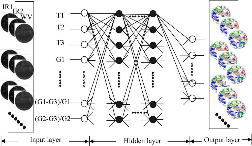
- Pre-processing: Download FY-2C level 1 data of June, July and August in 2007 in HDF format. Then prepare underlying surface map and the Tbb map of three infrared channels (IR1, 10.3–11.3 μm; IR2, 11.5–12.5 μm and WV 6.3–7.6 μm).
- Data visualization: According to its time stamp order, open FY-2C Tbb maps of three infrared channels and underlying surface map at the same time with special human-computer interactive software. The software is developed by Dr. Cang-Jun Yang in NSMC (National Satellite Meteorological Center in Beijing) in the Window PC environment.
- Pixel Sample collection: Scan image and find out a cloud patch whose cloud type is desired, such as cumulonimbus (Cb), thick cirrus according to the experience of our invited meteorological experts. Then choose one pixel at the center of the cloud patch and record its related information: Tbb of IR1, IR2, and WV. This method only chooses one pixel in one cloud patch, and it discards indecipherable cloud patches even with expert’s eyes. Therefore, the samples collected in this study are clearly defined typical cloud types and can be deemed as “truth”. Repeat the sample pixel collection process for the whole image.
- Sample Database establishment: Repeat step 2 and 3. In this study, we collect about 15 pixel samples at one timestamp from the multi-channel images. There are about 200-timestamp multi-channel images have used and 2864 samples of cloud types have been collected. These samples covered almost all types of the geographical regions which are spread over mountains, plains, lakes, and coastal areas. These samples were collected during different period of the day to account the diurnal features of clouds. The number of sample pixels for each category of surface/clouds is shown in Table 2.
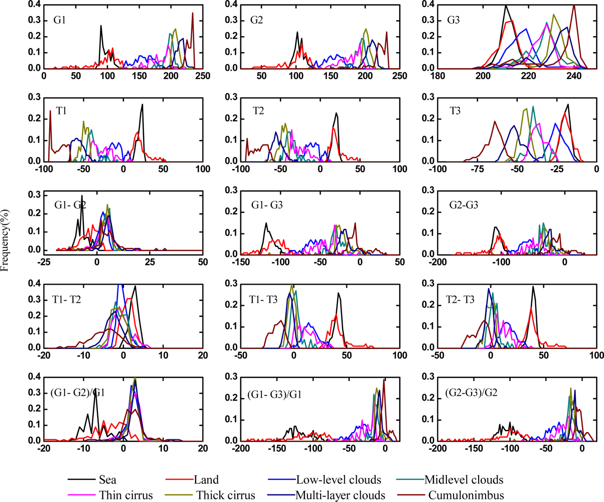
2.4. Features
2.5. Reasonableness Test of Samples
2.6. Configuration
3. Methodology
3.1. Cloud Classifier
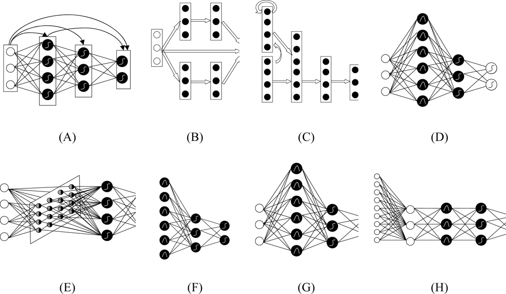
3.1.1. Brief Description of Cloud Classifiers
- Back Propagation (BP): BP (Figure 3A) is probably the most widely used algorithm for generating classifiers. It is a feed-forward multi-layer neural network [33]. It has two stages: a forward pass and a backward pass. The forward pass involves presenting a sample input to the network and letting activations flow until they reach the output layer. The activation function can be any function. During the backward pass, the network’s actual output (from the forward pass) is compared with the target output and error estimates are computed for the output units. The weights connected to the output units can be adjusted in order to reduce those errors. The error estimates of the output units can be used to derive error estimates for the units in the hidden layers. Finally, errors are propagated back to the connections stemming from the input units.
- Modular Neural Networks (MNN): MNN (Figure 3B) is a special class of Multilayer perceptron (MLP). These networks process their input using several parallel MLPs, and then recombine the results. This tends to create some structure within the topology, which will foster specialization of function in each sub-module.
- Jordan-Elman Neural Networks: Jordan and Elman networks (Figure 3C) extend the multilayer perceptron with context units, which are processing elements (PEs) that remember past activity. In the Elman network, the activity of the first hidden PEs is copied to the context units, while the Jordan network copies the output of the network. Networks which feed the input and the last hidden layer to the context units are also available.
- Probabilistic Neural Network (PNN): PNN (Figure 3D) is nonlinear hybrid networks typically containing a single hidden layer of processing elements (PEs). This layer uses Gaussian transfer functions, rather than the standard Sigmoid functions employed by MLPs. The centers and widths of the Gaussians are set by unsupervised learning rules, and supervised learning is applied to the output layer. All the weights of the PNN can be calculated analytically, and the number of cluster centers is equal to the number of exemplars by definition.
- Self-Organizing Map (SOM): SOM (Figure 3E) transforms the input of arbitrary dimension into one or two dimensional discrete map subject to a topological (neighborhood preserving) constraint. The feature maps are computed using Kohonen unsupervised learning.
- Co-Active Neuro-Fuzzy Inference System (CANFIS): The CANFIS model (Figure 3F) integrates adaptable fuzzy inputs with a modular neural network to rapidly and accurately approximate complex functions. Fuzzy inference systems are also valuable as they combine the explanatory nature of rules (membership functions) with the power of “black box” neural networks.
- Support Vector Machine (SVM): SVM (Figure 3G) has been very popular in the machine learning community for the classification problem. Basically, the SVM technique aims to geometrically separate the training set represented in an Rn space, with n standing for the number of radiometric and geometric criteria taken into account for classification, using a hyperplane or some more complex surface if necessary. SVM training algorithm finds out the best frontier in order to maximize the margin, defined as a symmetric zone centered on the frontier with no training points included, and to minimize the number of wrong classification occurrences. In order to reach that goal, SVM training algorithm usually implements a Lagrangian minimization technique. It reduces complexity for the detection step. Another advantage is its ability to generate a confidence mark for each pixel classification based on the distance measured in the Rn space between the frontier and the point representative of the pixel to be classified: the general rule is that a large distance means a high confidence mark. In this study, the SVM is based upon a training set of pixels with known criteria and classification (cloud/surface). It is implemented using the Kernel Adatron algorithm. The Kernel Adatron maps inputs to a high-dimensional feature space, and then optimally separates data into their respective classes by isolating the inputs which fall close to the data boundaries. Therefore, the Kernel Adatron is especially effective in separating sets of data which share complex boundaries.
- Principal Component Analysis (PCA): PCA (Figure 3H) is a very popular technique for dimensionality reduction. It combines unsupervised and supervised learning in the same topology. In this study, we use PCA to extract principal features of cloud image. These features are integrated into a single module or class. This technique has the ability to identify relatively fewer “features” or components that as a whole represent the full object state and hence are appropriately termed “Principal Components”. Thus, principal components extracted by PCA implicitly represent all the features.
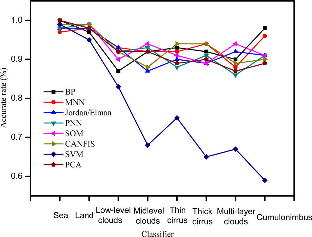
3.1.2. Comparison of Cloud Classifiers
3.2. Evaluation Indices for Model Parameters Screening and Model Testing
3.2.1. Mean square error (MSE):
3.2.2. Normalized mean square error (NMSE):
3.2.3. Percent Error (%):
3.2.4. Correlation coefficient (Corr) :
3.2.5. Accuracy rate (%)
3.2.6. Akaike’s Information Criterion (AIC):
3.2.7. Rissanen’s Minimum Description Length (MDL):
3.3. Cloud Classifier Parameters
3.4. Training and Validation of Cloud Classifier
4. Result and Analysis
4.1. Pixel-level Evaluation of Classification Results
4.1.1. Cross-Examination Results of Classification
4.1.2 Test Results of Classification
4.1.3. Comparison with FY-2C Operational Cloud Classification Products
4.2. Cloud path-Level Evaluation of Classification Results
4.2.1. Case 1: high latitude case
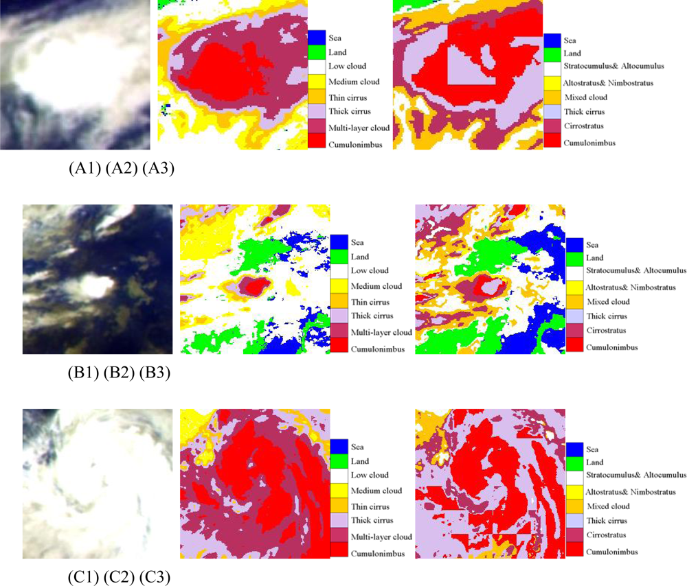
4.2.2. Case 2: Cumulonimbus case
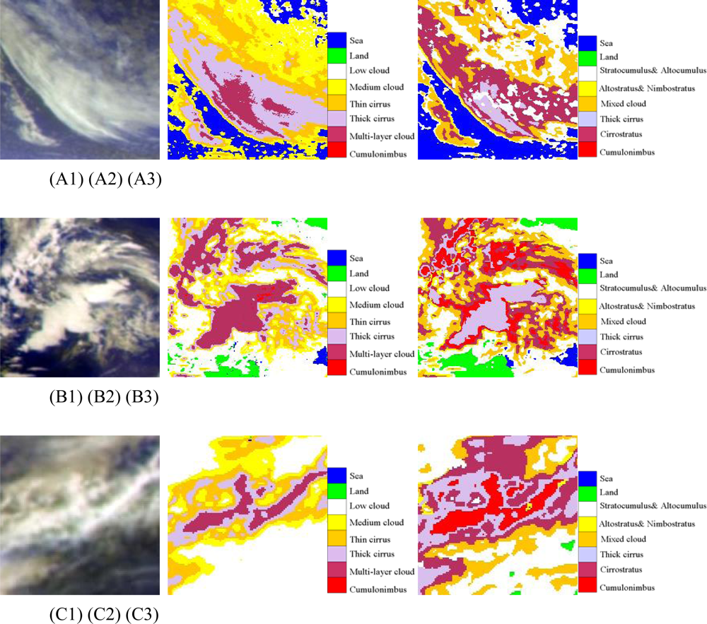
4.2.3. Case 3: Cirrus case
5. Conclusions and Discussion
Acknowledgments
References and Notes
- Hobbs, P.V.; Deepak, A. (Eds.) Clouds: Their Formation, Optical Properties and Effects; Academic Press: New York, NY, USA, 1981; p. 285.
- Hunt, G.E. On the sensitivity of a general circulation model climatology to changes in cloud structure and radiative properties. Tellus 1982, 34, 29–38. [Google Scholar]
- Liou, K.N. Influence of cirrus clouds on weather and climate processes: a global perspective. Mon. Weather Rev 1986, 114, 1167–1199. [Google Scholar]
- Vázquez-Cuervo, J.; Armstrong, E.M.; Harris, A. The effect of aerosols and clouds on the retrieval of infrared sea surface temperatures. J. Climate 2004, 17, 3921–3933. [Google Scholar]
- Aha, D.W.; Bankert, R.L. Cloud classification using error-correcting output codes. Ai Applications 1997, 11, 13–28. [Google Scholar]
- Baum, B.A.; Tovinkere, V.; Titlow, J.; Welch, R.M. Automated cloud classification of global AVHRR data using a fuzzy logic approach. J. Appl. Meteorol 1997, 36, 1519–1540. [Google Scholar]
- Ackerman, S.A.; Strabala, K.I.; Menzel, W.P.; Frey, R.A.; Moeller, C.C.; Guclusteringey, L.E. Discriminating clear sky from clouds with MODIS. J. Geophys. Res 1998, 103, 141–157. [Google Scholar]
- Key, J. Cloud cover analysis with Arctic advanced very high resolution radiometer data. 2: Classification with spectral and textural measures. J. Geophys. Res 1990, 95, 7661–7675. [Google Scholar]
- Berendes, T.A.; Mecikalski, J.R.; MacKenzie, W.M., Jr.; Bedka, K.M.; Nair, U.S. Convective cloud identification and classification in daytime satellite imagery using standard deviation limited adaptive clustering. J. Geophys. Res 2008, 113(d20), D20207. [Google Scholar]
- Ebert, E.E. Analysis of polar clouds from satellite imagery using pattern recognition and a statistical cloud analysis scheme. J. Appl. Meteor 1989, 28, 382–399. [Google Scholar]
- Ruprecht, E. Statistical approaches to cloud classification. Adv. Space Res 1985, 5, 151–164. [Google Scholar]
- Key, J.; Maslanik, J.A.; Schweiger, A.J. Classification of merged AVHRR/3 and SMMR Arctic data with neural networks. Photogram. Eng. Remote Sens 1989, 55, 1331–1338. [Google Scholar]
- Uddstrom, M.J.; Gray, W.R.; Murphy, R.; Oien, N.A.; Murray, T. A Bayesian cloud mask for sea surface temperature retrieval. J. Atmos. Ocean. Technol 1999, 16, 117–132. [Google Scholar]
- Li, J.; Menzel, W.P.; Yang, Z.; Frey, R.A.; Ackerman, S.A. Highspatial- resolution surface and cloud-type classification from MODIS multispectral band measurements. J. Appl. Meteorol 2003, 42, 204–226. [Google Scholar]
- Berendes, T.A.; Kuo, K.S.; Logar, A.M.; Corwin, E.M.; Welch, R.M.; Baum, B.A.; Pretre, A.; Weger, R.C. A comparison of paired histogram, maximum likelihood, class elimination, and neural network approaches for daylight global cloud classification using AVHRR imagery. J. Geophys. Res. Atmos 1999, 104, 6199–6213. [Google Scholar]
- DaPonte, J.S.; Vitale, J.N.; Tselioudis, G.; Rossow, W. Analysis and classification of remote sensed cloud imagery. Proceedings of the International Conference on Applications and Science of Artificial Neural Networks III; Spie - Int Soc Optical Engineering: Orlando, FL, USA, 1997. [Google Scholar]
- Bischof, H.; Schneider, W.; Pinz, A.J. Multispectral classification of Landsat-images using neural networks. IEEE Trans .Geosci. Remote Sens 1992, 30, 482–490. [Google Scholar]
- Lee, J.; Weger, R.C.; Sengupta, S.K.; Welch, R.M. A neural network approach to cloud classification. IEEE Trans .Geosci. Remote Sens 1990, 28, 846–855. [Google Scholar]
- Shi, C.X.; Qu, J.H. NOAA-AVHRR cloud classification using neural networks. Acta Meteorol. Sin 2002, 13, 250–255. [Google Scholar]
- Azimi-Sadjadi, M.R.; Gao, W.F.; Vonder Haar, T.H.; Reinke, D. Temporal updating scheme for probabilistic neural network with application to satellite cloud classification - further results. IEEE Trans. Neural Networks 2001, 12, 1196–1203. [Google Scholar]
- Bankert, R.L. Cloud classification of AVHRR imagery in maritime regions using a probabilistic neural network. J. Appl. Meteor 1994, 33, 909–918. [Google Scholar]
- Azimi-Sadjadi, M.R.; Wang, J.; Saitwal, K.; Reinke, D. A multi-channel temporally adaptable system for continuous cloud classification from satellite imagery. IEEE Trans. Neural Networks 2001, 3, 1625–1630. [Google Scholar]
- Jiang, D.M.; Chen, W.M.; Fu, B.S.; Wang, J.K. A Neural network approach to the automated cloud classification of GMS imagery over South-east China maritime regions. J. Nanjing Inst. Meteorol 2003, 26, 89–96. (in Chinese).. [Google Scholar]
- De Silva, C.R.; Ranganath, S.; De Silva, L.C. Cloud basis function neural network: a modified RBF network architecture for holistic facial expression recognition. Patt. Recogn 2008, 41, 1241–1253. [Google Scholar]
- Zhang, W.J.; Xu, J.M.; Dong, C.H. China’s current and future metorolical satellite systems. In Earth Science Remote Sensing; TsingHua University Press: Beijing, China, 2007; Volume 1, pp. 392–413. [Google Scholar]
- Li, D.R.; Dong, X.Y.; Liu, L.M.; Xiang, D.X. A new cloud detection algorithm for FY-2C images over China. International Workshop on Knowledge Discovery and Data Mining (WKDD), Adelaide, Australia, 2008; pp. 289–292.
- Ebert, E. A pattern recognition technique for distinguishing surface and cloud types in Polar Regions. J. Climate Appl. Meter 1987, 26, 1412–1427. [Google Scholar]
- Garand, L. Automated recognition of oceanic cloud patterns. Part I: Methodology and application to cloud climatology. J. Climate 1988, 1, 20–39. [Google Scholar]
- Reed, R.D.; Marks, R.J. Neural Smithing: Supervised Learning in Feed forward Artificial Neural Networks; MIT Press: Cambridge, MA, USA, 1999. [Google Scholar]
- Bajwa, I.S.; Hyder, S.I. PCA based image classification of single-layered cloud types. J. Market Forces 2005, 1, 3–13. [Google Scholar]
- Azimi-Sadjadi, M.R.; Zekavatl, S.A. Cloud classification using support vector machines. Geosci. Remote Sens. Sym 2000, 2, 669–671. [Google Scholar]
- Wang, H.J.; He, Y.M.; Guan, H. Application of support vector machines in cloud detection using EOS/MODIS – art; Report No. 70880M; Proceedings of the Conference on Remote Sensing Applications for Aviation Weather Hazard Detection and Decision Support; SPIE-Int. Soc. Optical Engineering: San Diego, CA, USA, 2008; pp. 880–880. [Google Scholar]
- Rumelhart, D.E.; Hinton, G.E.; Williams, R.J. Learning representation by BP Errors. Nature (London) 1986, 7, 149–154. [Google Scholar]
- Allen, R.C., Jr.; Durkee, P.A.; Wash, C.H. Snow/cloud discrimination with multispectral satellite measurements. J. Appl. Meteorol 1990, 29, 994–1004. [Google Scholar]


| Channel No. | Channel name | Spectral range (μm) | Spatial resolution (km) |
|---|---|---|---|
| 1 | IR1 | 10.3–11.3 | 5 |
| 2 | IR2 | 11.5–12.5 | 5 |
| 3 | IR3(WV) | 6.3–7.6 | 5 |
| 4 | IR4 | 3.5–4.0 | 5 |
| 5 | VIS | 0.55–0.90 | 1.25 |
| Classes | Samples | Description |
|---|---|---|
| Sea | 184 | Clear sea |
| Land | 266 | Clear land |
| Low-level clouds | 405 | Stratocumulus (Sc), Cumulus (Cu), Stratus (St), Fog, and Fractostratus (Fs) |
| Midlevel clouds | 379 | Altocumulus (Ac), Altostratus (As), and Towering Cumulus |
| Thin cirrus | 415 | Thin cirrus |
| Thick cirrus | 440 | Thick cirrus |
| Multi-layer clouds | 371 | Cumulus congestus (Cu con), Cirrostratus (Cs) and Cirrocumulus (Cc) |
| Cumulonimbus | 404 | Cumulonimbus(Cb) |
| Sum | 2864 |
| Features | Parameters | Description |
|---|---|---|
| Spectral features | T1,T2, T3 | Top brightness temperature of IR1,IR2,WV |
| Gray features | G1, G2, G3 | Gray value of IR1,IR2,WV |
| G1–G2, G1–G3, G2–G3 | ||
| Assemblage features | T1–T2, T1–T3, T2–T3 | The combination of infra split window and water vapor channel |
| (G1–G2)/G1, (G1–G3)/G1, (G2–G3)/G2 |
| Type of network | Output layer | Hidden layer | |||
|---|---|---|---|---|---|
| Learning step | Number of hidden layer | Number of Neurons | Learning step | ||
| ANN | BP | 0.10 | 2 | 9,4**(1) | 0.10 |
| MNN | 0.10 | 1 | 4,4**(2) | 0.10 | |
| Jordan/Elman***(1) | 0.10 | 1 | 9 | 0.10 | |
| PNN***(2) | 1.00 | 1 | 6 | 1.00 | |
| SOM Network***(3) | 0.10 | 1 | 9 | 1.00 | |
| CANFIS***(4) | 0.10 | 1 | 4 | 0.10 | |
| SVM | 0.01 | ||||
| PCA***(5) | 0.10 | ||||
| Cross-examination (Training) | Test | ||||||||||||
|---|---|---|---|---|---|---|---|---|---|---|---|---|---|
| Method | Time(S) | MSE | NMSE | Corr | Errol (%) | AIC | MDL | MSE | NMSE | Corr | Errol (%) | AIC | MDL |
| BP | 30.00 | 0.01 | 0.02 | 0.99 | 9.35 | −399.35 | −214.35 | 0.01 | 0.02 | 0.99 | 8.87 | −2693.14 | −3376.66 |
| MNN | 21.00 | 0.02 | 0.05 | 0.98 | 9.20 | −106.53 | −46.16 | 0.01 | 0.03 | 0.99 | 8.87 | −2832.60 | −2599.99 |
| Jordan/Elman | 22.00 | 0.01 | 0.03 | 0.99 | 8.75 | −31.27 | −126.34 | 0.02 | 0.03 | 0.99 | 8.88 | −3852.71 | −3398.99 |
| PNN | 63.00 | 0.01 | 0.03 | 0.99 | 8.52 | 2812.18 | 3428.47 | 0.01 | 0.02 | 0.99 | 7.75 | −20.61 | 2160.85 |
| SOM | 21.00 | 0.03 | 0.05 | 0.98 | 8.92 | 854.12 | 947.30 | 0.01 | 0.02 | 0.99 | 7.74 | −1340.14 | −699.23 |
| CANFIS | 44.00 | 0.02 | 0.04 | 0.98 | 10.53 | 464.56 | 924.43 | 0.02 | 0.03 | 0.99 | 9.23 | −4851.31 | −3776.72 |
| SVM | 22.30 | 0.67 | 2.01 | −0.08 | 49.82 | 38837.55 | 4820.26 | 0.67 | 2.01 | −0.08 | 49.82 | 38837.55 | 48200.26 |
| PCA | 19.00 | 0.02 | 0.03 | 0.99 | 10.42 | −46.33 | −48.75 | 0.01 | 0.02 | 0.99 | 10.18 | −1449.86 | −1293.18 |
| Type | FY2C product | ANN cloud classification |
|---|---|---|
| Sea | 83.02 | 99.01 |
| Thick Cirrus | 26.14 | 88.79 |
| Cumulonimbus | 76.49 | 90.74 |
| Land | 48.35 | 98.51 |
© 2009 by the authors; licensee MDPI, Basel, Switzerland This article is an open access article distributed under the terms and conditions of the Creative Commons Attribution license (http://creativecommons.org/licenses/by/3.0/).
Share and Cite
Liu, Y.; Xia, J.; Shi, C.-X.; Hong, Y. An Improved Cloud Classification Algorithm for China’s FY-2C Multi-Channel Images Using Artificial Neural Network. Sensors 2009, 9, 5558-5579. https://doi.org/10.3390/s90705558
Liu Y, Xia J, Shi C-X, Hong Y. An Improved Cloud Classification Algorithm for China’s FY-2C Multi-Channel Images Using Artificial Neural Network. Sensors. 2009; 9(7):5558-5579. https://doi.org/10.3390/s90705558
Chicago/Turabian StyleLiu, Yu, Jun Xia, Chun-Xiang Shi, and Yang Hong. 2009. "An Improved Cloud Classification Algorithm for China’s FY-2C Multi-Channel Images Using Artificial Neural Network" Sensors 9, no. 7: 5558-5579. https://doi.org/10.3390/s90705558
APA StyleLiu, Y., Xia, J., Shi, C.-X., & Hong, Y. (2009). An Improved Cloud Classification Algorithm for China’s FY-2C Multi-Channel Images Using Artificial Neural Network. Sensors, 9(7), 5558-5579. https://doi.org/10.3390/s90705558