Article

Pattern Recognition and Pathway Analysis with Genetic Algorithms in Mass Spectrometry Based Metabolomics

UC Davis Genome Center, 451 Health Sciences Drive, Davis, CA 95616-8816, U.S.A
*
Author to whom correspondence should be addressed.
Algorithms 2009, 2(2), 638-666; https://doi.org/10.3390/a2020638
Submission received: 20 October 2008 / Revised: 2 February 2009 / Accepted: 26 March 2009 / Published: 3 April 2009
(This article belongs to the Special Issue Algorithms and Molecular Sciences)

Abstract

:
A robust and complete workflow for metabolic profiling and data mining was described in detail. Three independent and complementary analytical techniques for metabolic profiling were applied: hydrophilic interaction chromatography (HILIC–LC–ESI–MS), reversed-phase liquid chromatography (RP–LC–ESI–MS), and gas chromatography (GC–TOF–MS) all coupled to mass spectrometry (MS). Unsupervised methods, such as principle component analysis (PCA) and clustering, and supervised methods, such as classification and PCA-DA (discriminatory analysis) were used for data mining. Genetic Algorithms (GA), a multivariate approach, was probed for selection of the smallest subsets of potentially discriminative predictors. From thousands of peaks found in total, small subsets selected by GA were considered as highly potential predictors allowing discrimination among groups. It was found that small groups of potential top predictors selected with PCA-DA and GA are different and unique. Annotated GC–TOF–MS data generated identified feature metabolites. Metabolites putatively detected with LC–ESI–MS profiling require further elemental composition assignment with accurate mass measurement by Fourier-transform ion cyclotron resonance mass spectrometry (FT-ICR-MS) and structure elucidation by nuclear magnetic resonance spectroscopy (NMR). GA was also used to generate correlated networks for pathway analysis. Several case studies, comprising groups of plant samples bearing different genotypes and groups of samples of human origin, namely patients and healthy volunteers’ urine samples, demonstrated that such a workflow combining comprehensive metabolic profiling and advanced data mining techniques provides a powerful approach for pattern recognition and biomarker discovery.

1. Introduction

The notions of system biology and personalized medicine are expected to change our views of health and diseases fundamentally in the near future. The term “system biology” has been coined to integrate data generated by all the “omics” platforms, taking advantage of the fast pace of the IT industry. Currently there are challenges highlighting in each realm of “omics”. In metabolomics studies, samples were highly complex, biologically variable, and with large dynamic range, challenging separation, detection, and data analysis. Multiple techniques have been be used in metabolomics, such as nuclear magnetic resonance spectroscopy (NMR), gas chromatography-mass spectrometry (GC-MS), liquid chromatography-mass spectrometry (LC-MS), and capillary electrophoresis-mass spectrometry (CE-MS), each with its own advantages and drawbacks. For all of the metabolites with different polarity and in a wide molecular weight range, the combination of these techniques is needed.
NMR is a non-destructive analytical technique, and sample preparation for NMR is straightforward and largely automated, but it is difficult to analyze NMR spectra of complex mixtures and NMR has a relative low sensitivity in the micro-molar range. Comparing to detectors such as NMR, MS provides better sensitivity and selectivity, and wider range of covered metabolites, at the benefit of the invention of electro-spray ionization (ESI) and atmosphere pressure chemical ionization (APCI). Direct-injection MS analyzes large number of metabolites in a very short time. However, direct infusion is hampered by ion suppression and matrix effects, where the signal of many analytes with low ionization efficiencies cannot be detected. To avoid these problems, MS is often hyphenated to GC or LC to decrease sample complexity.
GC-MS is a sensitive and robust separation technique with established applications in the field of Metabolomics [4]. However, GC technique is not suitable for analysis of large or thermo labile compounds such as nucleotides or oligosaccharides. LC-MS usually does not require derivatization, has many modes of separation, and comes with a large sample loading capacity. Reversed-phase chromatography (RP) is a mature technique for separation of non-polar compounds. Monolithic capillary columns [5,6,7,8,9,10,11] and ultra performance liquid chromatography (UPLC) [12] have introduced high chromatographic peak resolution to LC, which in the past could be reached only by capillary GC columns. However, RP is not easily applicable to separate highly polar compounds. Ion-exchange chromatography is regularly used to separate organic anions and carbohydrates, but coupling to mass spectrometry (MS) is difficult due to high concentrations of non-volatile inorganic salts in the mobile phases. Hydrophilic interaction chromatography (HILIC) is recommended to separate simple and complex carbohydrates, amino acids, glycosides, and other polar natural products [13,14,15,16,17,18,19,20]. Coupling the separation techniques briefly described above to mass spectrometry (MS) provides extremely versatile and valuable tools for metabolomics studies [10,11,15,21,22].
Datasets generated with these techniques require modern computational tools and robust data mining technologies [23,24]. Unsupervised methods, such as principle component analysis (PCA), are well-established techniques for dimensionality reduction and visualization, where the extracted information is represented by a set of new variables, termed as components [24]. In order to select prominent potential biomarkers among all the peaks, supervised methodologies with built-in preprocessing and feature selection are needed [26,27,28]. Feature selection, also known as variable selection, feature reduction, attribute selection or variable subset selection, is a technique commonly used in machine learning to select a subset of relevant feature for building robust learning models [29]. There are two major categories of feature selection, univariate and multivariate methods. Univariate methods test one metabolite at a time for its ability to discriminate a dependent variable, then, top most significant metabolites are used to develop a statistical model. Multivariate methods take into consideration the synergy among metabolites. Based on different subsets of metabolites, many possible models are evaluated and the most predictive model is identified and selected [30,31]. It was reported [32] that Genetic Algorithms (GA) are promising multivariate approach in analysis of the LC–ESI–MS metabolomics datasets.
Genetic Algorithms approach is inspired by the features of real biological systems. It is, actually, a tool for feature/variable/predictor selection in data mining. The GA procedure starts from random populations of metabolites subsets of a given size [33]. Each subset is assessed for its ability to predict disease effects and has a certain level of accuracy. A new generation of subsets with higher classification accuracy is produced by mechanisms mimicking natural selection such as reproduction, selection, mutation, crossover, and migration. These new subsets replace the initial population, and the progressive improvement of the subset population is repeated enough times until a desired level of accuracy is reached. A major difference between GA and other machine learning approaches is its ability to determine relationship among feature components, providing valuable information about metabolite interactions, metabolic pathways, and clinical diagnosis. However, in order to better understand metabolic networking data, major breakthroughs are needed in the following challenging areas: high-throughput de novo identification; integrated mapping of microarray, proteomics, metabolomics, and biological knowledge base; robust and flexible computational methodologies to calculate cluster coefficients and similarities between metabolic networks in relation to subtle changes in environmental, biochemical or developmental conditions.
In present study we applied GA on pattern recognition and pathway analysis among datasets generated by three complementary analytical MS based techniques in three different cases. GC–TOF–MS data were annotated prior further analysis. LC–ESI–MS data were not annotated. Unsupervised methods and supervised methods were used for data processing as well.

2. Results and Discussion

2.1 General workflow
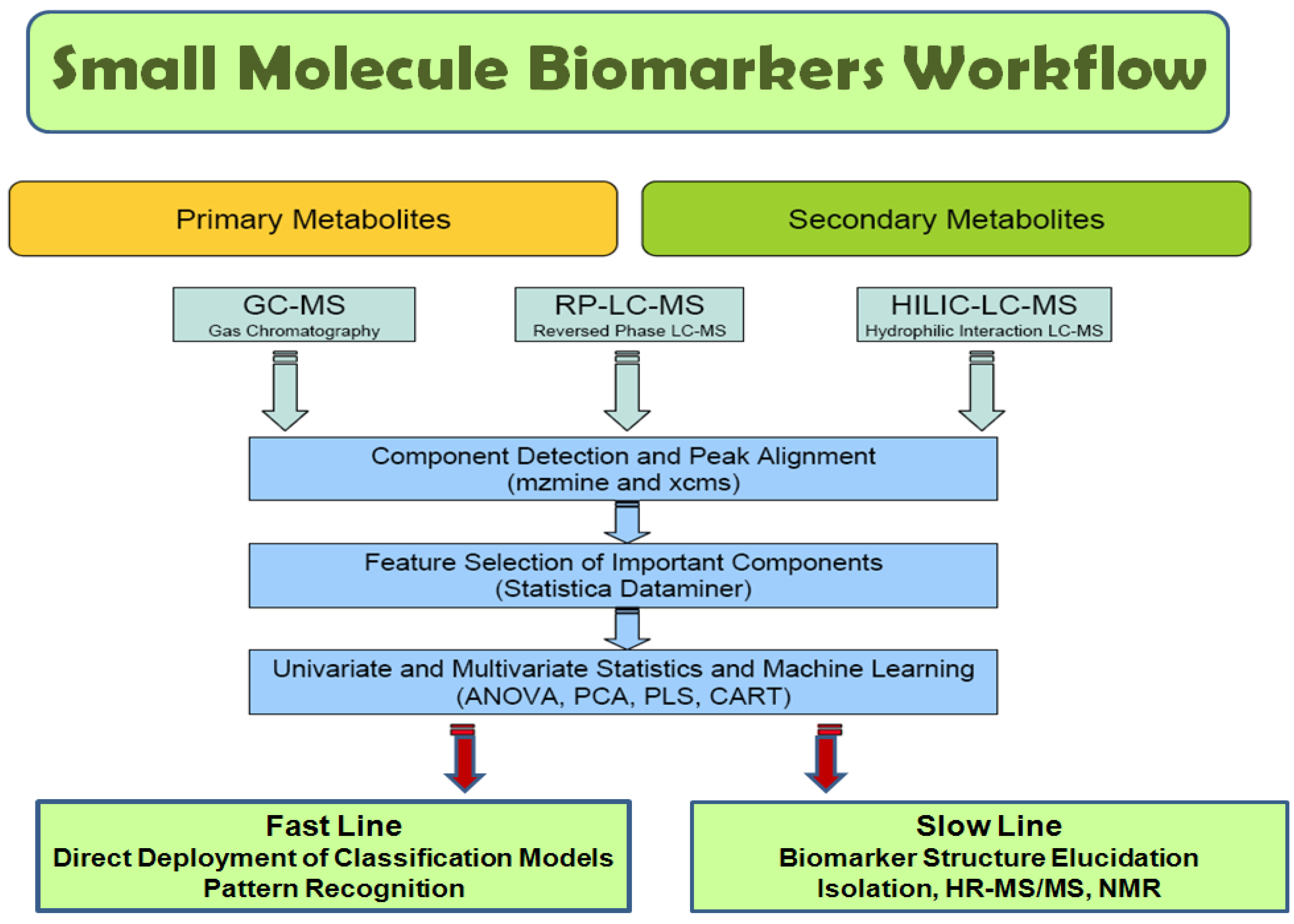
The scheme of the workflow on small molecules is illustrated in Figure 1. General steps were data acquisition, annotation, pre-processing, PCA exploration, manual or GA feature selection, classification and prediction, and pathway construction [34].
Figure 1. Small Molecule Analysis Workflow at UC Davis Metabolomics Core.
Algorithms 02 00638 g001
Depending on particular project univariate analysis may precede feature selection which is necessary in case processing of noisy data. In this case univariate analysis is used for irrelevant data finding and removal. This is true for LC-MS data.

2.1.1 Data acquisition (LC-MS)

It is known that LC-MS tuning is important to achieve better sensitivity, ionization efficiency, etc. [34]. Untargeted metabolic profiling requires full scan event efficiency of which depends on a single general tune file used. Five different compounds were used to determine the best tuning used for profiling: sucrose, rutin, naringin, indoleacetic acid and chlorogenic acid. Data mining with the use of comprehensive statistics allowed convincingly discriminate data obtained with the use of different tune files (data not shown). Small molecules were the most sensitive to the different tune files while larger sized polar lipids were less sensitive to described alterations. It was found that the sucrose tune file was the most appropriate one for the reason of its better metabolites’ response in both positive and negative ESI modes [34], so the sucrose tune file was used in the MS methods applied to the current study. Data acquisition on LTQ linear ion trap MS (ThermoFinnigan, San Jose, CA) was performed in full scan featuring constant positive and negative modes switching. This allowed monitor positive and negative ions within a single LC-MS run.

2.1.2 Data annotation

GC–TOF–MS data were annotated prior further analysis [35,36]. LC–ESI–MS data were not annotated. The GC-MS annotation procedure was automated with the data output generated as an Excel table [35,36]. Initial GC–TOF–MS peak detection and mass spectrum deconvolution were performed with ChromaTOF software (version 2.25, Leco). A reference chromatogram was defined that had a maximum of detected peaks over a signal/noise threshold of 20 and used for automated peak identification based on mass spectral comparison to a standard NIST 05 library and in-house customized mass spectral libraries. Analytes spectra were searched against custom spectrum libraries and identified based on retention index and spectrum similarity match. A mixture of the retention time standards, n-dodecane (RI 1,200), n-pentadecane (RI 1,500), n-nonadecane (RI 1,900), n-docosane (RI 2,200), n-octacosane (RI 2,800), n-dotriacontane (RI 3,200), and n-hexatriacontane (RI 3,600) was included in the final reagent volume [37]. Automated assignments of unique fragment ions for each individual metabolite were chosen as quantifiers, and manually corrected where necessary. Relative quantification was performed on quantifiers with optimal selectivity. All known artifact peaks caused by column bleeding or phthalates and polysiloxanes derived from MSTFA hydrolysis were manually identified and removed from the results table.
Since the purposes of the described studies were mainly clustering, classification, and prediction, termed as the fast track of the workflow (Figure 1), metabolite annotation and identification were not required prior data mining. Putative biomarkers presented as feature LC-MS peaks are subjects for further analysis by FT-ICR-MS and/or LC-FT-ICR-MS for accurate mass measurement, isotopic abundance pattern, MS/MS fragmentation pattern, and/or FT-NMR for spatial structure elucidation, termed as the slow track of the workflow (Figure 1).

2.1.3 Data pre-processing

R-based XCMS [38], Java-based Mzmine, and commercially available MarkerView [39,40] were used for pre-processing in current study. Because Mzmine took almost one week for analyzing a relatively small dataset, suggesting time consuming calculations, XCMS and MarkerView were preferred.
Each chromatogram was manually inspected on the presence of repetitive noise, artifacts and solvents inclusions. Each blank and QC chromatograms were used for ruling out data that do not belong to samples. The peak detection algorithm used by XCMS is based on cutting the LC/MS data into slices a fraction of a mass unit (0.1 m/z) wide and then operating on those individual slices in the chromatographic time domain. Within each slice, the signal is determined by taking the maximum intensity at each time point in the slice. After identifying peaks in individual samples, those peaks must then be matched across samples to allow calculation of retention time deviations and relative ion intensity comparison. XCMS incorporated a peak-matching algorithm that takes into account the two-dimensional, anisotropic nature of LC/MS data. The XCMS retention time alignment algorithm simultaneously corrects the retention times of all samples in a single step. After XCMS parameter optimization, the group bandwidth was set to 30, the minimum fraction was set to 0.5, the minimum sample parameter was set to 1, the width of overlapping m/z values was set to 0.5, and the maximum number of groups in a single m/z slice was set to 0.5.
After processing and peak picking, mass spectral features were retrieved from XCMS as a TXT file. The dataset was normalized using Euclidean norm by scaling each sample-vector to unit vector norm, which can be interpreted geometrically as a projection of the samples x to a hyper-sphere with the length of this sample vector scaled to one. After normalization, the ratios between masses are the same as before, but the intensity of the sample is removed. Since unit variance unifies the influence of each variable, vector normalization is closely related to correlation analysis. Because unmodified PCA is a linear method and vector norm projects to a curved hyperspace, theoretically, the normalized data could be linearized by transforming from Cartesian to spherical coordinates, where the angles have hierarchical orders. However, this does not affect the results very much. In practice, peaks were normalized to the total absolute area of all detected metabolites in each sample using an in-house written R script.

2.1.4 Unsupervised Analysis without Feature Selection

Mutation, natural variation, and environmental conditions affect metabolic processes. Metabolome analysis can help us to understand the link between these factors and the overall characteristics of an organism. Unsupervised methods are the choices to investigate underlying data structure, unbiased by the knowledge of experimental design. For LC-MS data, PCA and clustering were used for preliminary data mining on whole sets of peaks detected by XCMS and MarkerView. GC–TOF–MS datasets were used after annotation. Searching and elimination of correlated variables introduced by the samples preparation and/or analytical methods applied is very important especially when it concerns values close to the margins of measurements like overload, limits of detection and background noise levels. Close proximity to both these factors can easily generate false positive values characterized with the convincing p-value that may actually not reflect real situation, but the absence of the particular variable which is not detected in a sample, or group of samples, since its level is below current instrument/method lower limit of detection. When biological question is related to the highest variance in the dataset, PCA is a powerful technique for dimensionality reduction, visualization and exploration.
Visualization methods are often the best way to discover interesting grouping information in the data, whereas clustering methods provide mathematical rigor. Basically, there are three major categories of clustering methods: partitioning (clusters), hierarchical (trees), or probability model-based (models). Partitioning methods map peaks into multiple disjointed clusters using a chosen criterion. K-means is the most popular partitioning method, although it requires the input of an initial clustering number. The K-means clustering algorithm chooses a pre-specified number of cluster centers to minimize the within-class sum of squares from those centers. Hierarchical methods construct a binary tree in which the root is a single cluster containing only one element and the leaves each contain only one element. A divisive tree is top-down built and an agglomerative tree is bottom-up built. Recently, probability model-based clustering methods have become increasingly popular, with the advances in methods, software, and interpretability of the results. Probability modeling assumes that the data pool is a mixture with all of the labels lost and tries to find the most possible label for each data point.

2.1.5 Feature Selection Using GA

Feature selection facilitates data visualization and data understanding, reduces the measurement and storage requirements, reduces training and utilization time, and improves prediction performance. Feature selection methods can be classified into two categories. If the feature selection process does not involve a learning algorithm, it is a filter approach; otherwise it is a wrapper approach. Filter methods such as variable ranking are widely used because of their simplicity, scalability, and good empirical success. Sophisticated wrapper methods improve predictor performance compared to simpler variable ranking methods. Wrapper methods are remarkably simple and universal by utilizing the learning machine of interest as a black box to score subsets of variable according to their predictive power. Search strategies include best-first, branch-and-bound, simulated annealing, and genetic algorithms, using a validation set or cross-validation to assess performance. GA is a good feature selection algorithm because it automatically selects a small number of feature metabolites during evolutionary learning process, and it easily constructs an optimal prediction model with a small number of feature metabolites [33]. In addition, GA calculates the network connections among featured components, makes metabolic pathway analysis possible. A general GALGO pipeline has four major stages:
  • GA procedure initially creates chromosomes that are subsets of variables;
  • Fitness of each subset was defined as its ability to predict the group membership of each sample in the dataset, and the GA assigns a score to each subset;
  • GA procedure selects the fittest subset; this fittest subset generates more numerous offspring;
  • Two randomly selected parent subsets are used to create two new subsets mimicking biological crossover and mutation mechanisms; the process is repeated from stage 2 until an accurate subset is obtained.
The GA parameters were optimized: the nearest centroid classification method was applied, the maximum solutions value was set as 2,000 to stabilize top 20 feature components, the maximum generations value as 500 because thousands of generations would end up in over fitting, the goal fitness as 1.0, the subset (chromosome) size as 5, the population size as 20 plus an additional unit per each 400 variables, the mutation rate as 1 mutation per subset (chromosome), and the crossover value as all subsets (chromosomes) in exchange.

2.1.6 Classification and Prediction

The performance of the fittest GA model is used to predict validation sample sets. The fittest GA model for data predicted class memberships of validation samples with high sensitivity and specificity using nearest centroid analysis, confirming that the frequent components generated by GA are truly discriminative components and capable of predicting unknown samples. To make it clear, the sensitivity of the prediction for a given class k is defined as the proportion of samples in k that are correctly classified, whereas the specificity for a given class k is defined as the number of true negatives divided by the sum of true negatives and false positives.

2.1.7 Pathway Analysis

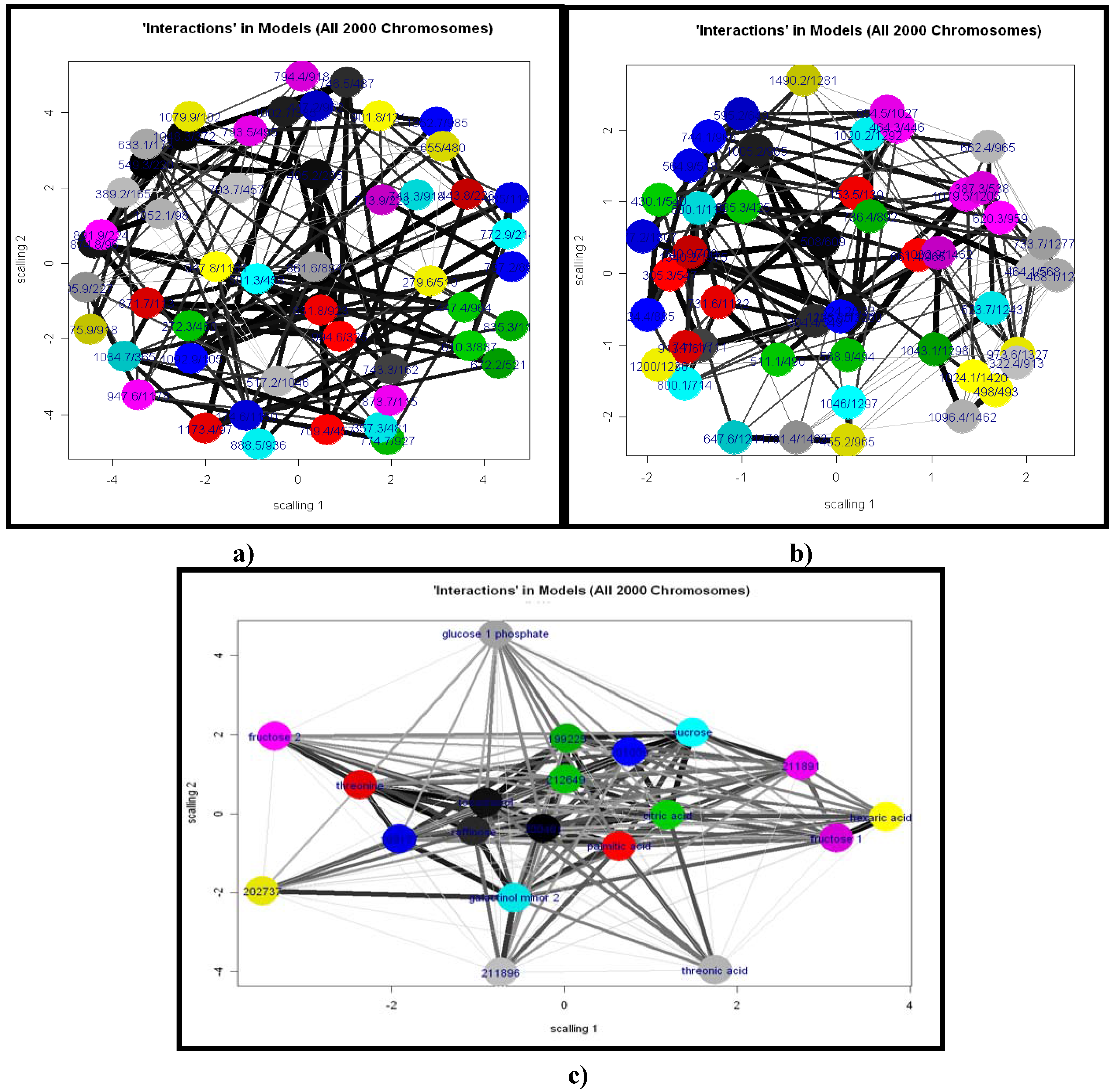
Figure 2a–c. Network interactions among feature components of the Pinus taeda L. HILIC (a), RP (b) LC–ESI–MS, and GC–TOF–MS (c) data. The line thickness represents the dependency strength relative to the population of relations shown. Top components were color-coded: the most frequent ones were black, then red, green, blue, cyan, pink, yellow, and gray. Predictors are described as mass to charge ratio which is unique characteristic of metabolite or chemical name for annotated metabolite.
Algorithms 02 00638 g002
A major difference between GA and other machine learning approaches is its ability to determine relationships among feature components, providing valuable information about metabolite interactions and metabolic pathways. The result of the evolutionary process of GA is a large pool of subsets of feature components. The models built on these subsets can be used for classification. In addition, associations can be identified through the most important feature components. The dependency of top-ranked GA selected feature components with each other was illustrated in Figures 2a–2c. The line thickness represents the dependency strength relative to the population of relations shown. By default, only the two most important dependencies per feature were shown. The authors understand that in order to get more complete information of biological pathways, these most important feature components have to be imported into specific pathway analysis software such as Cytoscape (http://www.cytoscape.org/), GeneGo (http://www.genego.com/) and/or Ingenuity (http://www.ingenuity.com/) Pathway Analysis tool. Here we demonstrate that even with the current correlation pathway analysis, preliminary hypothesis can be generated based on GA selected features/metabolites. Moreover, we believe that proposed pathways were the most affected ones. These proposed pathways are subjects for further targeted metabolomics study applying SRM/MRM techniques which provide much higher level of sensitivity and confidence.

2.1.8 GA Limitations

In addition to its requirement of intensive computation, GA as well as other machine learning methods has the limitation of over fitting data due to a large number of variables and a small number of cases in typical metabolomic studies [41]. Therefore, the predictors can be strongly biased toward the training set and generate poor prediction generality in “real-world” samples. If the fitness on the training data is significantly better than the fitness on the test data, it may indicate over fitting. In order to avoid over fitting, parameters have to be optimized and independent datasets are needed to validate the above predictors [41,42].

2.2 Examples

GA was used in three metabolomics datasets, as follows.

2.2.1 Plant samples

Identification of relationships between naturally occurring genetic and phenotypic variation in Pinus taeda L. Loblolly pine, a gymnosperm, may help to understand the evolution of adaptive traits in land plants [34]. In order to assign biological roles to genes of unknown function and to define gene networks of adaptive significance, a population genomic approach (association genetics) is used to study how allelic sequence variation among individuals results in phenotypic differences. Specifically, association at 1,000 loci allelic (SNP) variation with phenotypic variation is planned to investigate with the utilization of metabolic profiling technologies. Phenotypes will be measured in large populations of clonally propagated trees that represent the widest possible spectrum of genetic variation in the species. In the present study a pilot project is used as a simplified model allowing to approach/test and/or to develop sufficient methodologies for large-scale study.
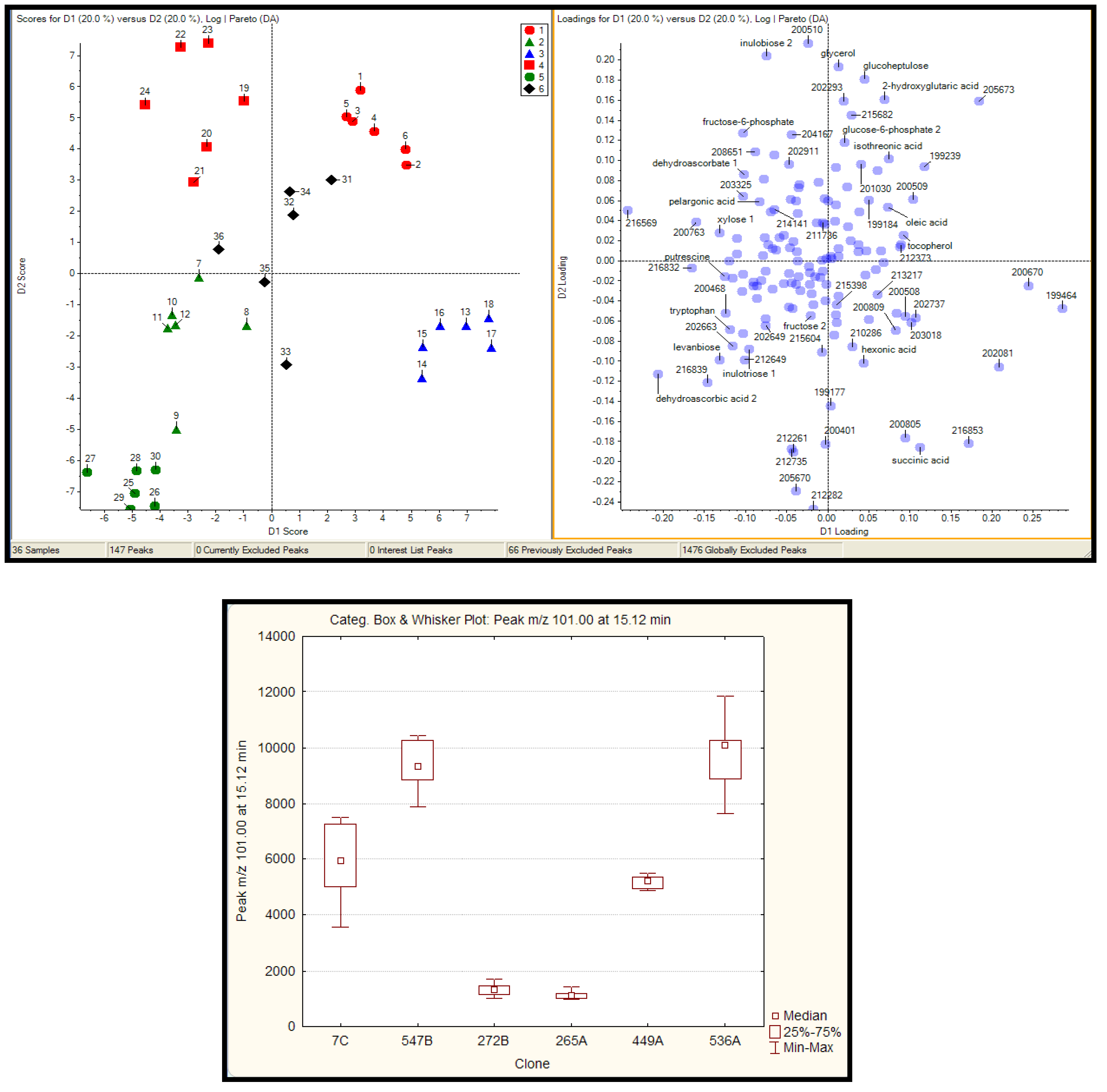
Six different clones of 1-year-old Pinus taeda L. seedlings grown under standardized conditions in a green house were used for sample preparation and further analysis [34]. In HILIC-LC/ESI-MS, RP-LC/ESI-MS, and GC/TOF-MS data, PCA plots showed significant clustering and differentiation among groups (Figure 3a, Figure 3b).
Figure 3a. Upper panel: PCA-DA score and loading plots of the Pinus taeda L. GC–TOF–MS data. Groups (clones) are color-coded in accordance with embedded legend. Software is MarkerView 1.0. Loading plot illustrate resolved annotated by BinBase [35,36]. Metabolites with chemical names assigned. Unidentified ones named by the numbers. Lower panel: variation of 4-O-galactopyranosyl-D-mannopyranose levels in different six clones.
Algorithms 02 00638 g003
Figure 3b. PCA-DA score plots of the Pinus taeda L. RP (left panel) and HILIC (right panel) LC–ESI–MS (B) datasets generated with MarkerView 1.0. Groups are color-coded in accordance with embedded legend.
Algorithms 02 00638 g004
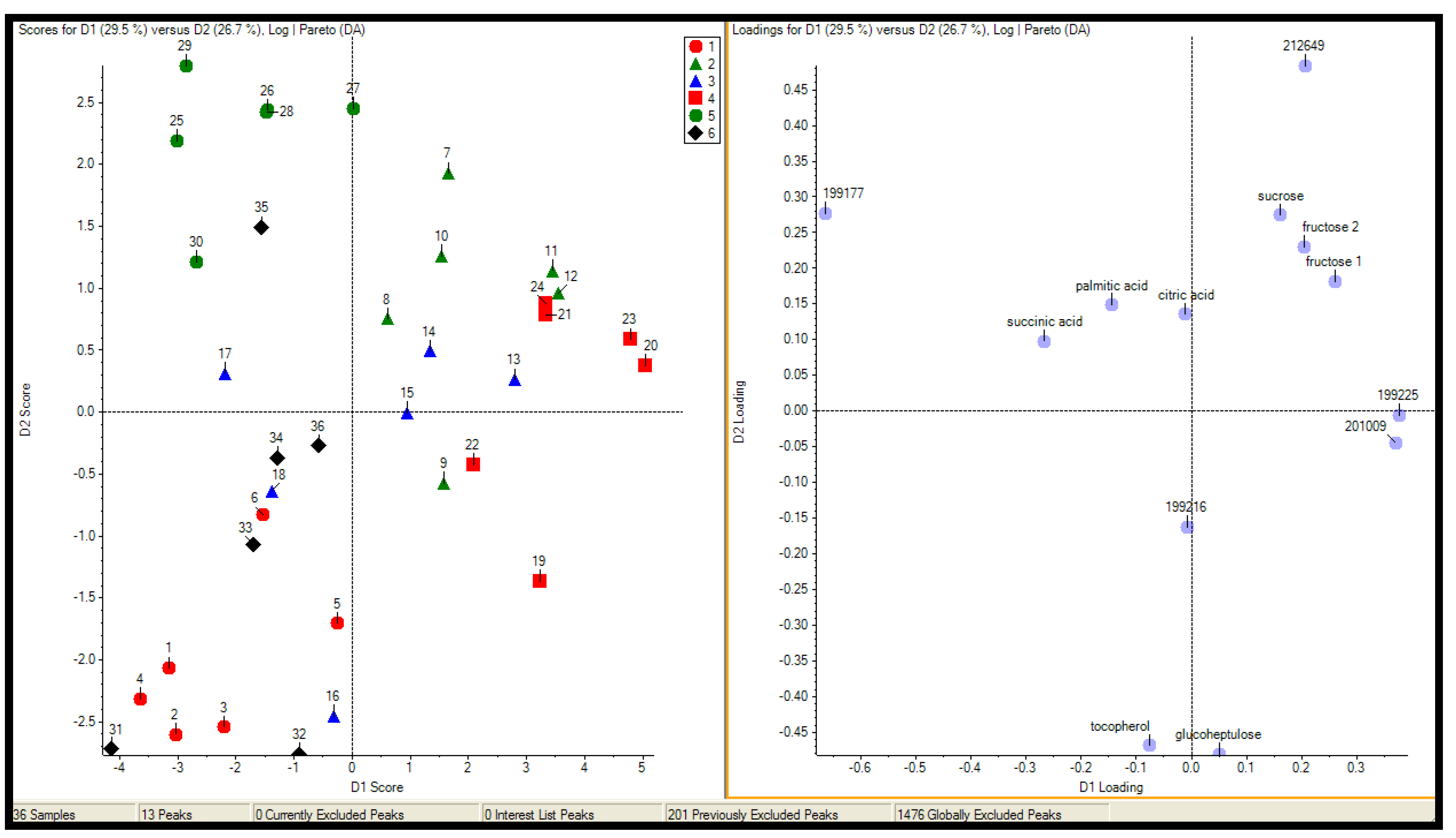
Figure 3c. PCA-DA score and loading plots generated with top 10 predictors derived by GA analysis.
Algorithms 02 00638 g005
When the cluster number was arbitrarily set as 6, kmeans and hclust functions showed similar results that group 1 and group 2 were mostly separated from the others. Without a priori knowledge of the cluster number, model-based mclust showed similar cluster numbers, while pvclust showed refined clustering structures. It seems that pvclust and mclust are good choices for clustering if grouping information is not available.
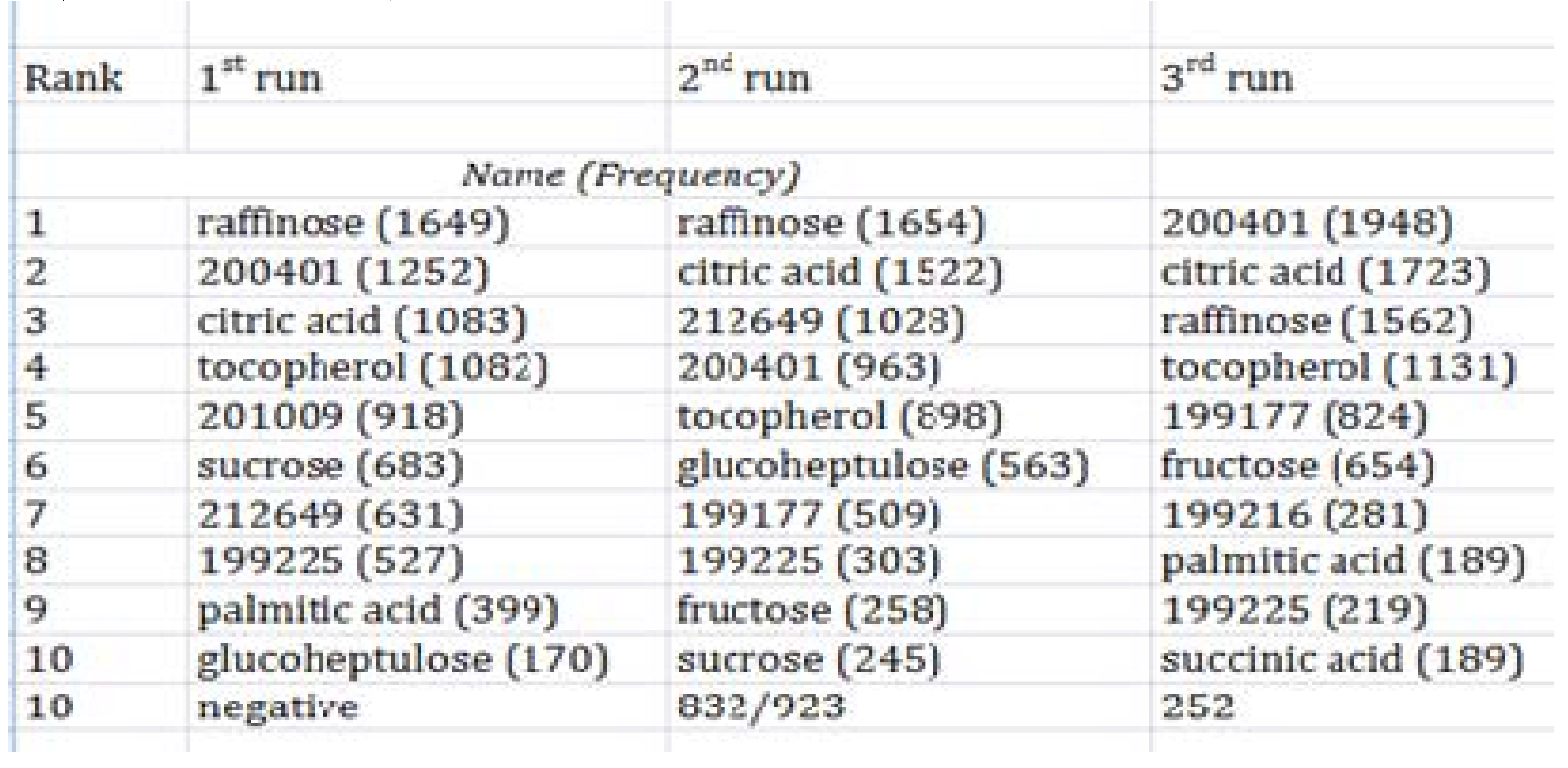
Since GA is stochastic and may give different solutions in each run or generation or model, the reproducibility of feature component selection across independent runs or models was tested. Frequencies, occurrences of feature components across different models generated from GA, were examined, and the results showed that a small set of components was frequently selected respectively (Table 1, Table 2, Table 3). It was found that 10 most frequent predictors in HILIC-LC/ESI-MS, RP-LC/ESI-MS, and GC/TOF-MS data occurred at least 100 times in 2000 models [34]. This observation suggests the potential importance of these components as discriminative for different genotypes. Another population of 2000 models generated by the second and third identical independent runs on the same GC/TOF-MS dataset showed that the top 10 component lists were very similar, although rank sequences were slightly different (Table 1).
Table 1. Top 10 classifiers from three identical independent runs on GC-TOF-MS data (Bin Base annotation).
Algorithms 02 00638 i001
Raffinose, tocopherol, citric acid, and compound 200401 always occurred in more than 1000 models out of the total 2000 models, suggesting that the top 10 component list would be more stabilized if enough GA solutions are allowed. For each model generated by GA, the GA procedure tests its prediction accuracy on the group membership of each sample in the dataset (fitness) and assigns a score. For HILIC, RP-LC/ESI-MS, and GC/TOF-MS data, a GA fitness solution was found within generation 200 in an average of all the models.
Table 2. Top 10 classifiers from HILIC-LC-ESI-MS and RP-LC-ESI-MS datasets (XCMS peak lists).
Algorithms 02 00638 i002
Table 3. Top 10 classifiers from HILIC-LC-ESI-MS and RP-LC-ESI-MS datasets (MarkerView 1.1 peak lists).
Algorithms 02 00638 i003
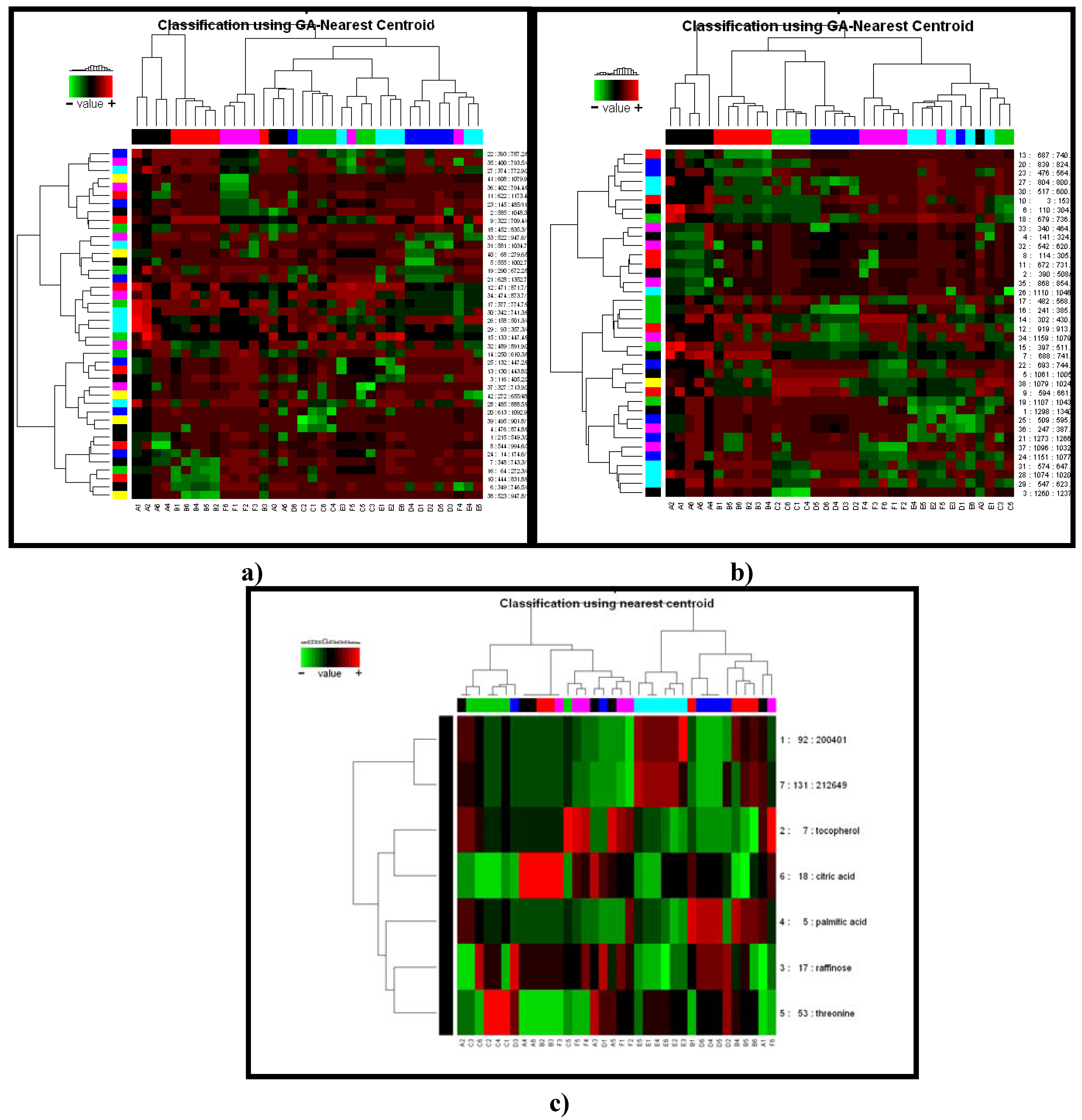
Because the GA procedure starts with a large number of subsets of components so that it provides a large collection of models, a single subset of components representative of the population is needed for prediction. Using GC/TOF-MS as an example, model number 1 was chosen for its highest classification accuracy and lowest number of feature components. The fittest model selected seven feature components with the highest frequencies. Comparing this to that without feature selection, the 2D PCA plot based on the fittest GA model showed nice clustering (Figure 3c). The heat map of the fittest GA model showed clustering of samples and clustering of the featured components (Figures 4a, 4b, 4c).
Figure 4 a–c. Heat map plot of the fittest GA model showed better clustering/classification of HILIC (a), RP (b) LC–ESI–MS, and GC–TOF–MS (c) data in the Pinus taeda L. Predictors are described as mass to charge ratio which is unique characteristic of metabolite. Annotated predictors provided with substance name.
Algorithms 02 00638 g006
The respective fittest GA model predicted with a specificity range of 0.85 to 0.98 and a sensitivity range of 0.36 to 1.0 for GC/TOF-MS data, a specificity range of 0.87 to 0.99 and a sensitivity range of 0.66 to 0.94 for HILIC-LC/ESI-MS data, and a specificity range of 0.88 to 1.0 and a sensitivity range of 0.74 to 0.96 for RP-LC/ESI-MS data. The metabolite network graph illustrated that many saccharides were interwoven heavily, indicating that carbohydrate metabolic pathways were involved (Figures 2a-c).
Palmitic acid and tocopherol also showed strong connections to other molecules. Palmitic acid is a major provider of ATP under beta-oxidation in mitochondria, and long-chain fatty acids such as palmitic acid typically require an antioxidant such as tocopherol to prevent peroxidation. Based on the results of performed analysis, the network graph provides us with some rough ideas that the genotype difference affects mostly on energy-providing pathways, especially the TCA cycle and its intermediates and precursors. Since mitochondria is the major cellular organelle in which all these reactions occur, a logical hypothesis could be generated from our data mining results, for example that mitochondria biochemistry may be affected in Pinus taeda L. with such genotypes.

2.2.2 Case Summary

The described case having size of 6 x 6 = 36 samples was designed as pilot project for currently ongoing project which size is 1,500 samples. Goal of the current study was to demonstrate ability profiling platforms discriminate plant samples, bearing different native genotype. In the range of two hundreds of components were found distinctive in all three methods. PCA-DA (MarkerView 1.1) was found effective and informative in data visualization and prominent predictors’ manual selection. GA was found providing unique predictors in some way overlooked by PCA based manual selections (Figures 3a-c). GA was found providing interesting information on pathways illustrated with the metabolites detected (Figures 2a-c).

2.2.3 Human urine samples

Novel approaches to early diagnosis and therapy of kidney diseases are urgently needed from economical and from personal needs [22,43]. For example, renal cell carcinoma (RCC) is a heterogeneous group of diseases with at least four well-defined histological types. The most common type of kidney malignancy is clear cell RCC (ccRCC), which is frequently associated with mutations of the von Hippel-Lindau gene. Another example is polycystic kidney disease (PKD), a genetic disorder characterized by the growth of numerous cysts in the kidneys. In the United States, more than half a million people have PKD, and cystic disease is the fourth leading cause of kidney failure. Due to the fact that the urine contains metabolic signatures of many biochemical pathways, urine is ideally suited for metabolomic analysis, especially involving diseases of the kidney and urinary system.
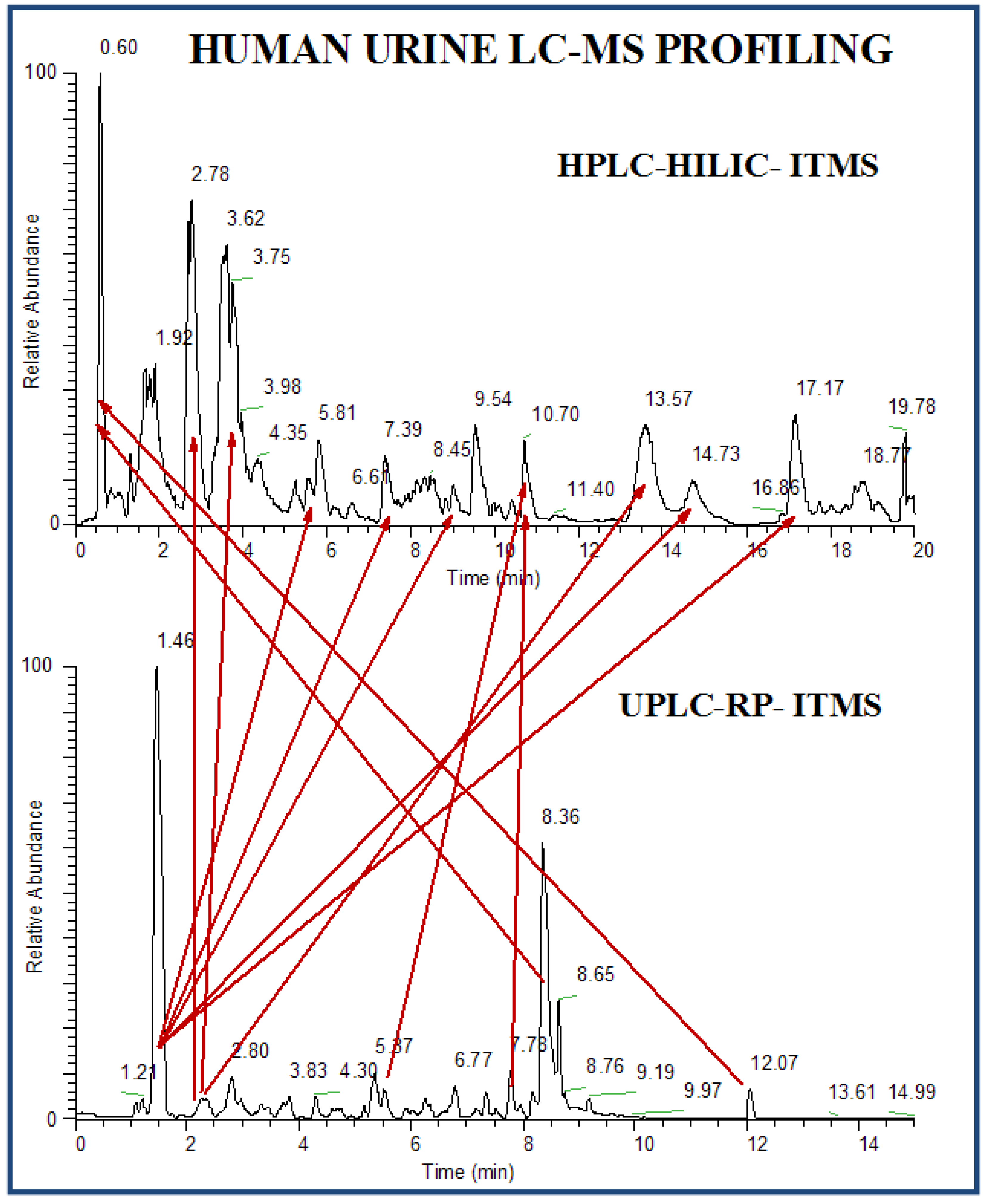
We have found that HILIC-LC-ESI-MS technique was more informative than the other two technology platforms in analyzing human urine samples in biomarkers discovery protocol for ccRCC and PKD cases. Therefore we currently present HILIC LC-MS generated results. The reason that HILIC LC-MS method was superior may be based on fact that the most compounds in human urine are water-soluble and are more suitable for HILIC- than for RP-LC separations (Figure 5).
Figure 5. Comparison of LC-MS chromatograms of human urine sample acquired in RP and HILIC chromatography modes on LTQ (linear ion trap mass spectrometer). Unresolved peaks in RP at Rt 1.46 min (lower panel) are resolved at different Rt in HILIC (upper panel). The same components illustrated as peaks (arrows depicted) were identified with measured parent ion masses to charge ratios and MS/MS fragmentation pattern similarity in both modes of acquisition: positive and negative.
Algorithms 02 00638 g007
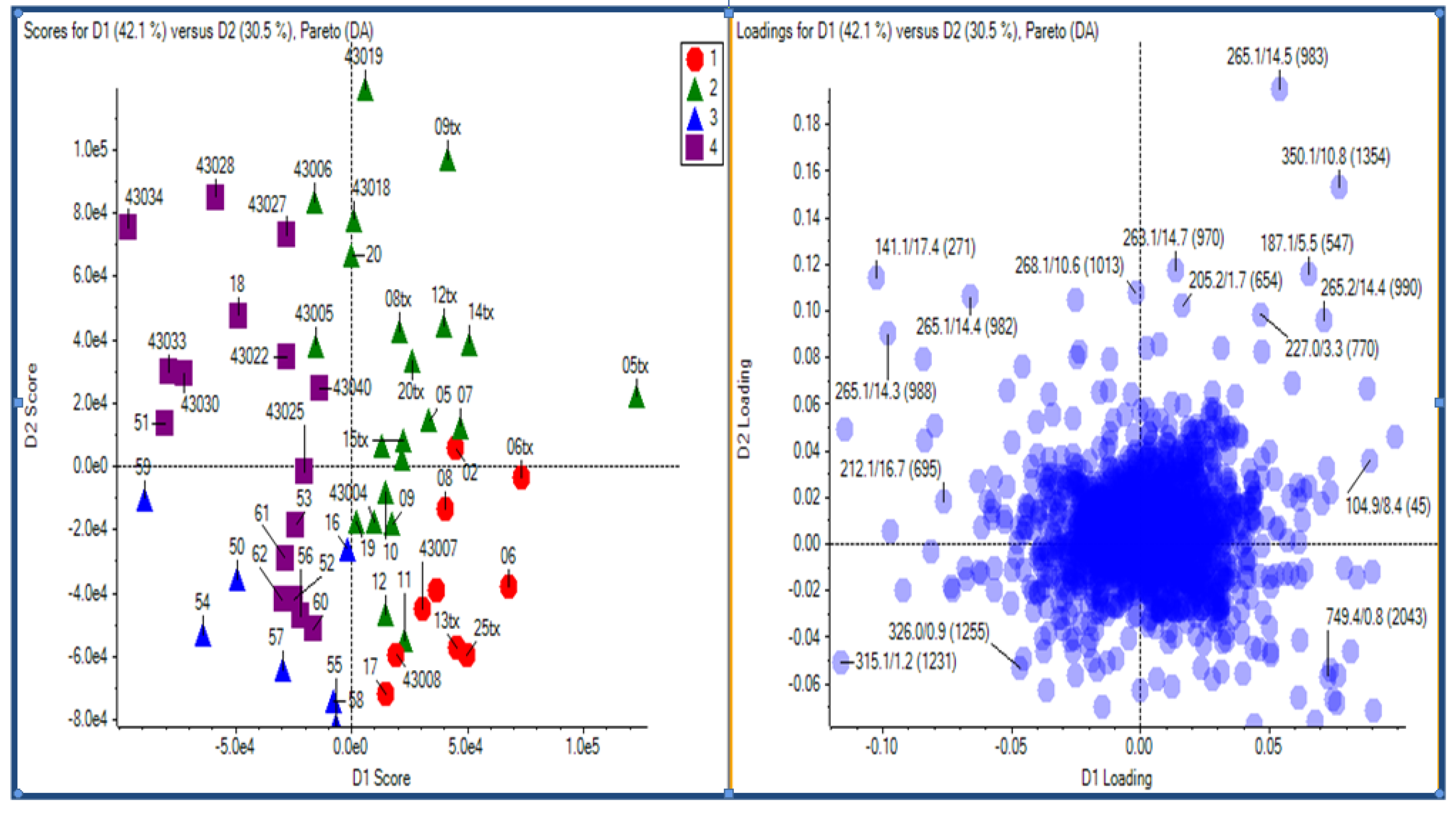
For the ccRCC HILIC dataset, the PCA plot by MarkerView showed that groups 1 (red) and 2 (green) were well separated from groups 3 (cyan) and 4 (blue), suggesting that ccRCC patients had different metabolism from healthy controls (Figure 6).
Figure 6. PCA-DA plot of the ccRCC HILIC-LC–ESI–MS before feature selection. Groups were color-coded as: 1-red: female ccRCC, 2-green: male ccRCC, 3-blue: female control, 4-purple: male control. Total of 55 samples, 2,111 predictors. Predictors (metabolites) characterized on PCA loading plots as mass to charge ratio / retention time / peak registry number. Sample number having tx extension originated from Texas, USA. Others are from Sacramento area, CA, USA. It is true for all presented PCA plots.
Algorithms 02 00638 g008
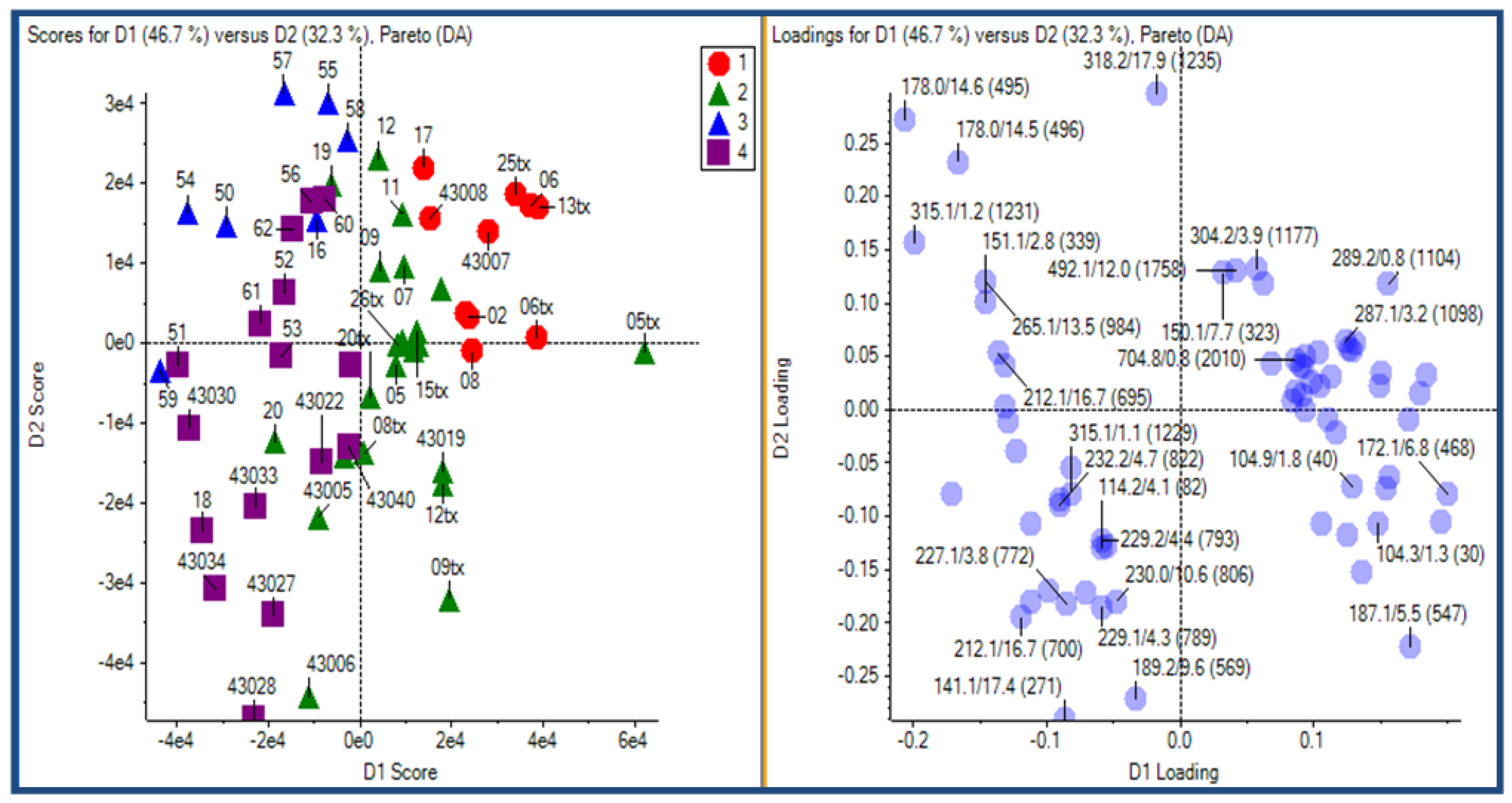
Both GA and manual feature selection approaches were applied to peak tables (potent predictors) generated with MarkerView 1.1 for LC/MS data. It was established that different feature peaks were found from the two independent feature selection approaches, whereas both were able to differentiate nicely RCC patients from healthy controls (Figure 7, Figure 8).
Figure 7. PCA-DA plot of the ccRCC HILIC-LC–ESI–MS after manual feature selection. Groups were color-coded as: 1-red: female ccRCC, 2-green: male ccRCC, 3- blue: female control, 4-purple: male control. 55 samples, 68 predictors.
Algorithms 02 00638 g009
Figure 8. PCA-DA plot of the ccRCC HILIC-LC–ESI–MS after GA feature selection. Groups were color-coded as: 1-red: female ccRCC, 2-green: male ccRCC, 3- blue: female control, 4-purple: male control. 55 samples, 22 predictors.
Algorithms 02 00638 g010
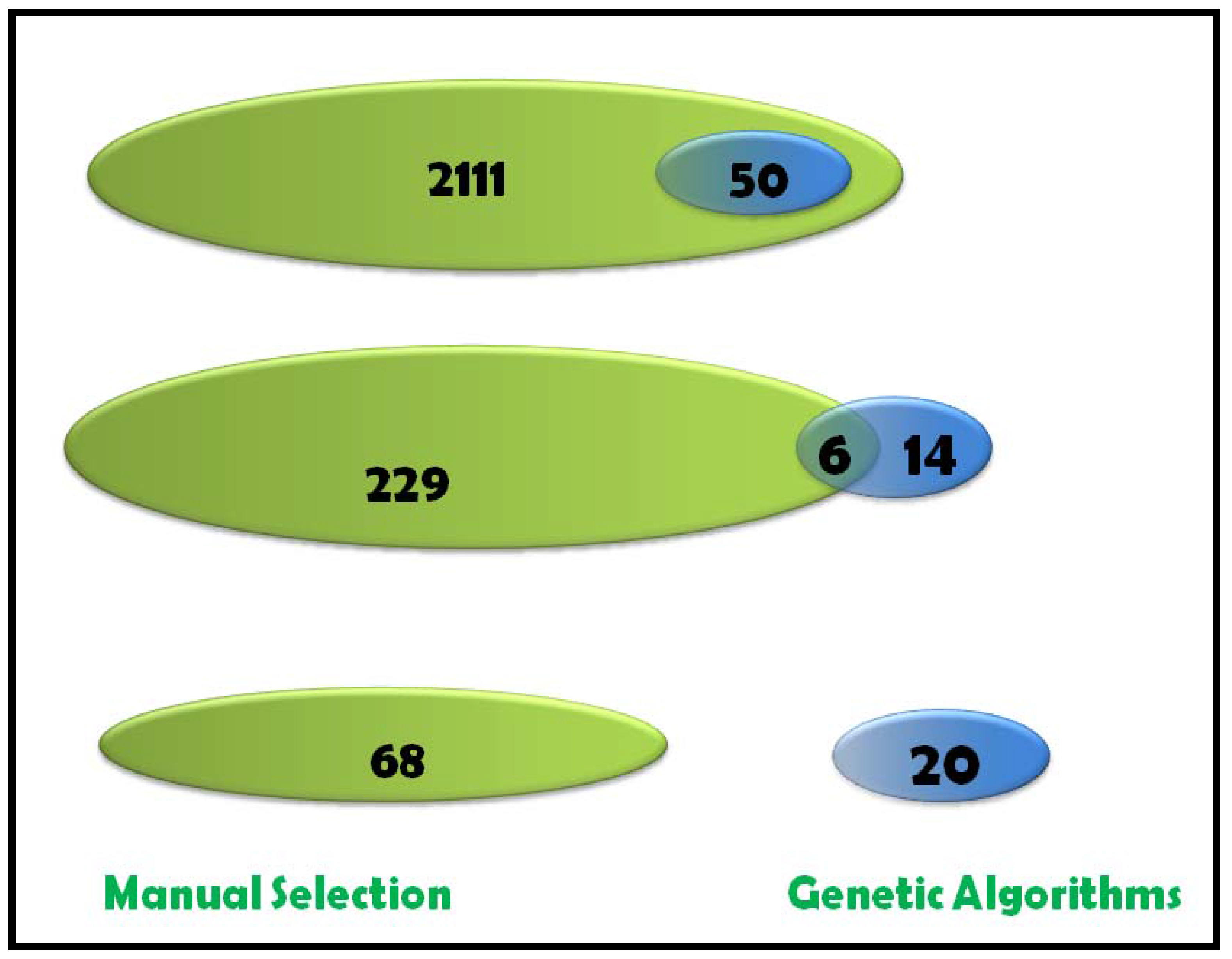
We have found that majority of GA selected predictors are minor and low abundant peaks, different from manually selected prominent predictors (Figure 9).
Figure 9. GA and manual feature selection methods generated two unique small subsets of highly potential predictors found during processing HILIC LC-MS data (ccRCC case).
Algorithms 02 00638 g011
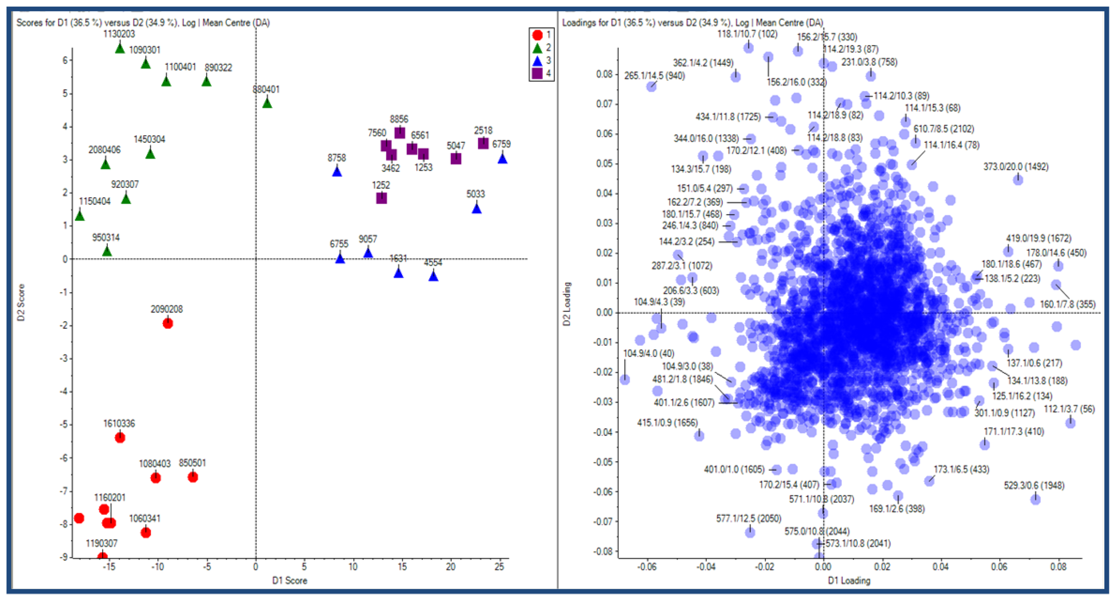
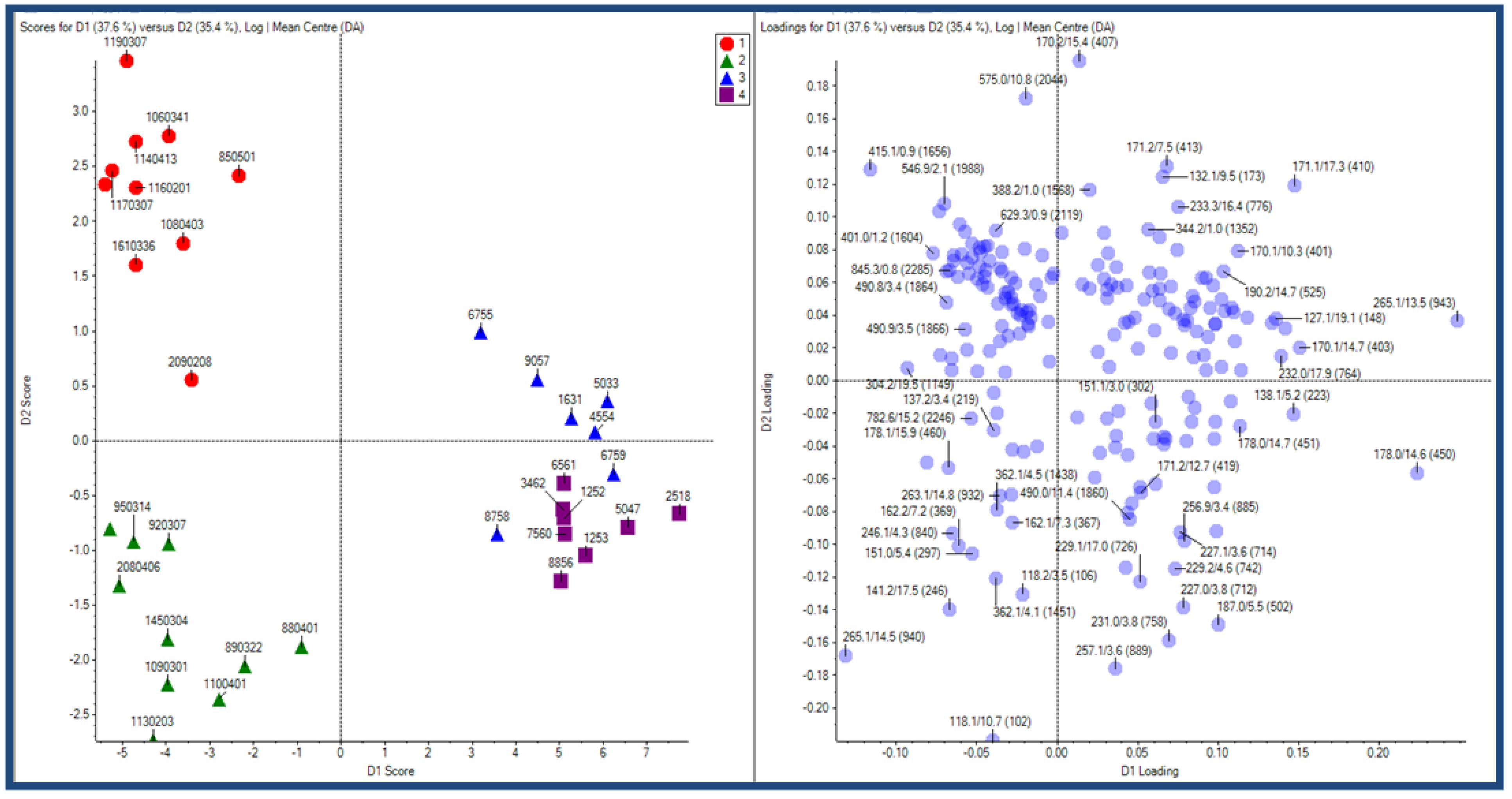
This observation is somewhat in accordance with our previous results and those described for NMR based metabolomics study where GA was applied for feature selection [34,44]. Similarly to describe above, PKD patients clearly differentiated from healthy controls on PCA-DA plots before and after GA or manual feature selection (Figure 10, Figure 11, Figure 12).
Figure 10. PCA-DA plot of the PKD HILIC-LC–ESI–MS before feature selection. Groups were color-coded as: 1-red: female PKD, 2-green: male PKD, 3-blue: female control, 4-purple: male control. Total 35 samples, 2,288 predictors.
Algorithms 02 00638 g012
Figure 11. PCA-DA plot of the PKD HILIC-LC–ESI–MS after manual feature selection. Groups were color-coded as: 1-red: female PKD, 2-green: male PKD, 3- blue: female control, 4-purple: male control. Total 35 samples, 206 predictors.
Algorithms 02 00638 g013
Figure 12. PCA-DA plot of the PKD HILIC-LC–ESI–MS after GA feature selection. Groups were color-coded as: 1-red: female PKD, 2-green: male PKD, 3- blue: female control, 4-purple: male control. Total 35 samples, 14 predictors.
Algorithms 02 00638 g014
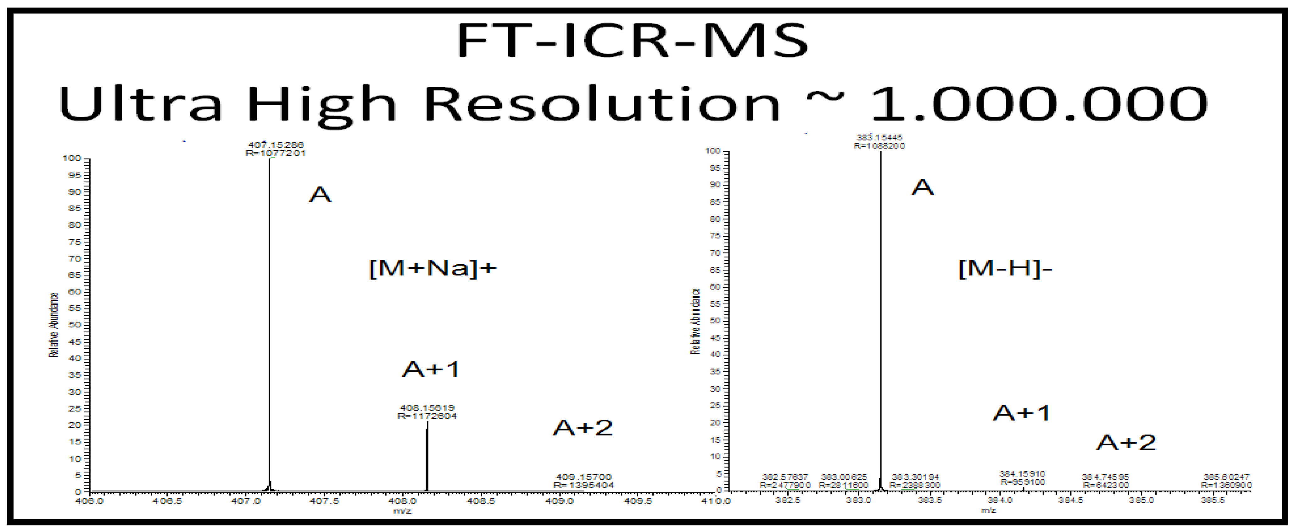
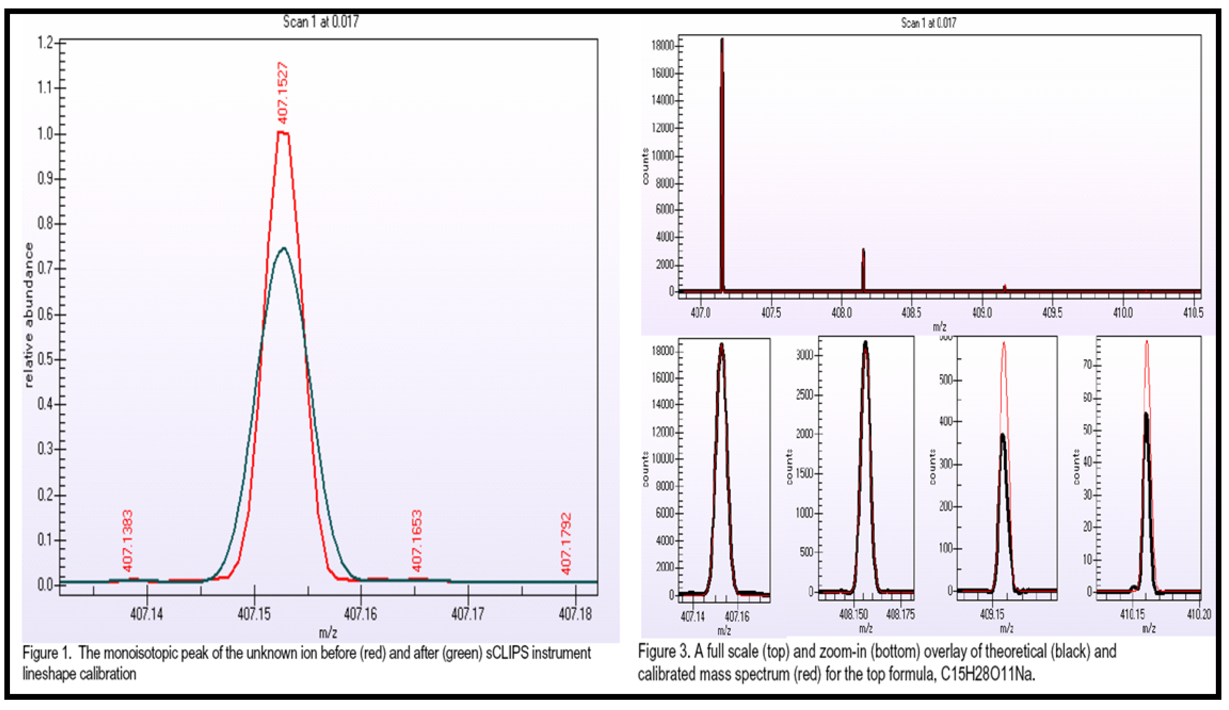
Interestingly genetically inherited PKD provides improved PCA-DA spatial groups separations compare to the same for RCC case. As we illustrated here, these features found are not meaningless numbers, but they are components possessing chemical identity (ID). As an example of selected component ID, we here present one of the compounds putatively identified utilizing high-resolution FT-ICR MS for accurate mass measurement, Mass WorksTM for spectral accuracy and isotopic abundance pattern, and Mass FrontierTM for fragmentation pattern (not shown) (Figure 13, Figure 14).
Figure 13. A high-resolution spectra of a potential predictor, m/z 407.1527 at positive mode [M+Na]+ and m/z 383.1545 at negative mode [M-H]-, illustrating isotopic pattern at 1,000,000 resolution using LTQ FT Ultra MS.
Algorithms 02 00638 g015
Figure 14. The unique elemental composition of m/z 407.1527 was assigned as C15H28O11Na using Mass WorksTM based on LC-MS data acquired using UPLC LTQ FT Ultra MS at 100,000 resolution.
Algorithms 02 00638 g016

2.2.4 Case Summary

The described case presents only two kidney diseases: acquired (ccRCC) and inherited (PKD). Final goal is early stage diagnostic test development. Initial study focus is on biomarkers discovery and validation. It was found that among three methods applied [22], HILIC LC-MS profiling is providing the most prominent biomarkers upon urine metabolic profiling (Figure 5) [43]. In the range of thousands of components were detected and found distinctive in all three methods. PCA-DA (MarkerView 1.1) was found effective and very informative in data visualization and manual selection. GA was found providing unique predictors in some way overlooked by PCA-DA based manual selections (Figure 6, Figure 7, Figure 8, Figure 10, Figure 11, Figure 12). A number of putative biomarkers were found during this data analysis reducing total number of candidates for diagnostic test development to the appropriate level which can be handled by reproducible analytical technique. Biomarkers identification and validation is the next step.

3. Experimental Section

3.1 Reagents and Standards

HPLC grade acetonitrile was purchased from Burdick and Jackson (VWR International, West Chester, PA). Each lot of organic solvents was investigated by LC–MS infusion. Extra pure ammonium acetate was purchased from EMD (Gibbstown, NJ). The ultrapure water was supplied by an in-house Millipore system (Billerica, MA). Fresh aqueous buffers for LC–ESI–MS were prepared on the working day. Methoxylamine hydrochloride, pyridine, N-methyl-N-trimethylsilyltrifluoro-acetamide (MSTFA), oligosaccharides kit, indole-3-acetic acid, sucrose, rutin, naringin, chlorogenic acid, and reserpine were purchased from Sigma-Aldrich (St. Louis, MO). For daily uses, MSTFA, pyridine, and/or reagents mix were stored in sealed aliquots under dry nitrogen after opening the bottle/ampoule or preparing the mix. A stock solution (1 mg/mL) of each tuning reference compound was prepared freshly on each working day in a solvent system identical to the initial mobile phase composition of LC. Reserpine stock solution was made 0.2 mg/mL in methanol. Oligosaccharide standards mix was prepared using oligosaccharides kit in acetonitrile: water (1:1, v.v.) with a concentration of 0.5 mg/mL for each component. Indole-3-acetic acid, sucrose, rutin, naringin, and chlorogenic acid solutions for MS tuning were prepared in acetonitrile: water (1:1, v.v.) with a concentration of 0.1 mg/mL.

3.2 Metabolomics Experimental Design and Sample Preparation

Nutritional and biorhythm effects can greatly complicate and confound metabolomics experiments. It is necessary to control the environment and state of the organism so that results can be explained with higher confidence. Sample preparation is critical for the success of metabolomic analysis. Tissue, organ, or fluid was deep flash frozen since response on sampling procedure quickly alters metabolism. The samples were flash frozen on liquid nitrogen and shipped on dry ice. Samples were stored at –80 oC until extraction and further analysis. Proteins were precipitated and removed, whereas proteins precipitation should not be harsh and abrupt since some of the small molecules associated/bound proteins co-precipitate and cannot be recovered. Consequent sample concentration was high enough to allow sufficient LC-MS column loading with the low injection volume. RP-LC separation does not require any processing of human urine samples, whereas neat urine was mixed with an equal volume of acetonitrile at room temperature for HILIC-LC-MS analysis. All samples were spun for 5 min at 13,000 rpm prior to injection for particles removal. More detailed experimental design and sample preparation procedures described previously [22,34,43].

3.3 LC–ESI–MS analysis

RP–LC–ESI–MS analysis of human urine samples was performed with the use of an ACQUITY UPLC system composed of a binary solvent manager, a sample manager, a column manager, and a TUV detector (Water Corp., Milford, MA). Although this configuration of UPLC hardware could reach as high as 15,000 psi, a working back pressure of 10,000 psi was targeted. A BEH C18 shielded column (1.7 μm, 150 x 2 mm) was used. Mobile phases used: A, ammonium acetate, 13 mM, pH 5.5; B, acetonitrile. After a 0.1 min isocratic run at 0% B, a gradient to 40% B was concluded at 8 min, and then it ramped at 95% B up to 9 min and maintained until 10.5 min. Following column wash was equilibration with 0% B at 11 min and maintained until 15 min. All injection volumes were 5 μL and column temperature was 35 °C, while the flow rate was 0.4 mL/min. Weak wash solvent was H2O-methanol (1:1, v/v) and strong wash solvent was acetonitrile-isopropanol (3:1, v/v).
HILIC–LC–ESI–MS analysis of human urine samples was performed with the use of a polyamine-bonded polymeric gel column (apHera NH2, 100 x 2 mm, 3 μm particle size, Advanced Separations Technologies, Whippany, NJ; apHera amino columns are based on covalently bonded strong alkaline compatible polyamine with a working pH range of 2 -13). The mobile phases were: acetonitrile (A), 13 mM ammonium acetate (pH 5.5, adjusted by acetic acid) (B), and 100 mM ammonium bicarbonate (pH 9.4, adjusted with ammonium hydroxide) (C) at the flow rates of 0.5 mL/min at 25oC. After a 1-min isocratic run at 5% B, a gradient to 35% B was concluded at 11 min, and then B was replaced by C starting at 50%, and gradient to 75% C was completed at 20 min. Following column wash the run was concluded with 100% C at 22 min. Column equilibration with starting buffer took 15 min before the next injection. The purpose of using mobile phase C at later stage of the gradient was to elute very polar compounds on the column. Since mobile phase C had a high pH value, a strong alkaline compatible HILIC column was used for this application. The injection volume was set to 5 μL. Weak wash solvent was acetonitrile-isopropanol (3:1, v/v) and strong wash solvent was H2O-methanol (1:1, v/v). For HILIC–LC–ESI–MS analysis, oligosaccharides were used as retention time indexes because they elute in the order of the increasing monomer units, with larger oligomers eluting as the latest ones. Mono and oligosaccharides were detected as ammonia adducts in positive mode and as [M-H]- ions in negative mode. The entire effluent from the HPLC column was directed into the electrospray ionization source (ESI) of a LTQ linear ion trap MS (ThermoFinnigan, San Jose, CA) operated under Xcalibur software (V1.4, ThermoFinnigan, San Jose, CA). The electrospray voltage was set to 5 kV. Nitrogen sheath and auxiliary gas flow was 60 and 20 arbitrary units respectively. The ion transfer capillary temperature was 350 °C. Typical ion gauge pressure was 0.90 ° 10-5. Full scan spectra were acquired from 150-850 amu at unit mass resolution with maximum injection time set to 200 ms in one micro scan. Acquisition was performed in both positive and negative switching modes. Sucrose tune file was used during all the LC–ESI–MS acquisitions on LTQ mass spectrometer. LC-MS protocols for the analysis of pine needles were described earlier [34].

3.4 GC–TOF–MS analysis

Briefly, neat urine samples were lyophilized without further pretreatment after our initial finding of severe alterations using urease treatments. Plant tissues were processed as described before [34]. To the dried samples 20 μL of 40 mg/mL methoxylamine hydrochloride in pyridine was added, and tubes with the samples were agitated at 30 °C for 30 min. Subsequently, 180 μL of trimethylsilylating agent N-methyl-N-trimethylsilyltrifluoroacetamide (MSTFA) was added, and samples were agitated at 37 °C for 30 min. GC–TOF–MS analysis was performed using an Agilent 6890 N gas chromatograph (Palo Alto, CA, USA) interfaced to a time-of-flight (TOF) Pegasus III mass spectrometer (Leco, St. Joseph, MI). Automated injections were performed with a programmable robotic Gerstel MPS2 multipurpose sampler (Mülheim an der Ruhr, Germany). The GC was fitted with both an Agilent injector and a Gerstel temperature-programmed injector, cooled injection system (model CIS 4), with a Peltier cooling source. An automated liner exchange (ALEX) designed by Gerstel was used to eliminate cross-contamination from sample matrix occurring between sample runs. Multiple baffled liners for the GC inlet were deactivated with 1-μL injections of MSTFA. The Agilent injector temperature was held constant at 250 °C while the Gerstel injector was programmed (initial temperature 50 °C, hold 0.1 min, and increased at a rate of 10 °C/s to a final temperature of 330 °C, hold time 10 min). Injections of 1 μL were made in split (1:5) mode (purge time 120 s, purge flow 40 ml/min). Chromatography was performed on an Rtx-5Sil MS column (30 m × 0.25 mm i.d., 0.25 μm film thickness) with an Integra-Guard column (Restek, Bellefonte, PA). Helium carrier gas was used at a constant flow of 1 mL/min. The GC oven temperature program was 50 °C initial temperature with 1 min hold time and ramping at 20 °C/min to a final temperature of 330 °C with 5 min hold time. Both the transfer line and source temperatures were 250 °C. The Pegasus III TOF (Leco, St. Joseph, MI) mass spectrometer ion source operated at –70 kV filament voltage with ion source. After a solvent delay of 350 s, mass spectra were acquired at 20 scans per second with a mass range of 50 to 500 m/z.

3.5 Raw Data Processing and Statistical Data Mining

The Xconvert program included in Xcalibur was used to convert the Xcalibur (*.raw) files to netCDF (*.cdf) format. Automatic peak finding, deconvolution, and alignment were performed using XCMS running on the open statistical platform R [38]. Preliminary data exploration was accomplished using unsupervised methods such as principle component analysis (PCA) and clustering. For PCA, a scree plot (to show the optimal number of eigenvalues), a score plot (to show the most important principal components and visually detect clusters), and a loading plot (to show positive and negative correlations of components) were included for each analysis using R package pcaMethods in Bioconductor project [45,46]. Cluster analysis of the PCA scores was performed using partitioning methods such as K-means using the function kmeans() in R package stats, hierarchical agglomerative methods such as Ward's method using the function hclust() in R package stats, and multiscale bootstrap resampling using R package pvclust, and model-based clustering approach using R package mclust which assumes a variety of data models and applying maximum likelihood estimation and Bayes criteria to identify the most likely model and number of clusters.
Genetic Algorithms (GA) are a class of algorithms based on the principle of biological evolution, suitable for finding approximate solutions to global optimization problems when there is a very large pool of possible solutions. The GA procedure incorporates operators such as biological inheritance, mutation, selection, and recombination on chromosomes, initial sets of candidate solutions [33]. Starting from a randomly generated set of subgroups and a criteria function for evaluating the fitness of an individual subset, GA procedure repeatedly selects the fittest candidate solutions in each generation and lets them reproduce and keep the population size constant. This process stops when the goal fitness is achieved. Goal fitness is defined as the average reachable fitness in a reasonable amount of generations. Feature selection using GA procedure and further classification were performed using R package GALGO [33]. With the equipment of hardware and software used, 2 days for 1 run using GA with nearest centroid method and the optimized parameter set were required to fulfill the task.
All calculations were performed in an R integrated development environment (IDE) RKWard under Kubuntu 7.10, a Debian Linux operating system, on a quad core Dell OptiPlex 755 workstation (4 x 3.0 GHz CPU speed, 2 x 4 MB L2 cache, 8 GB RAM). The current versions of Kubuntu, R, Bioconductor, XCMS, pcaMethods, stats, pvclust, mclust, GALGO, and RKWard are free open source software (FOSS).
The MarkerView 1.1 Software (Applied Biosystems/MDS Sciex, Concord, Ontario, Canada) [39,40] is designed to allow the data from several samples to be compared so that differences can be identified; typical applications include: metabolomics, biomarker discovery, metabolite identification, impurity profiling, etc. This software was used for data analysis in parallel to described above techniques in current study. The program uses multivariate analysis techniques to compare the samples and provides both supervised and unsupervised methods. Supervised methods use prior knowledge of the sample groups (for example, affected/altered vs. control) to determine the variables that distinguish the groups. In contrast, unsupervised methods allow the structure within the data to be determined and visualized. The two approaches can be combined, i.e. unsupervised methods can be used to determine the groups, and then supervised methods can be used to confirm the important variables.

3.6 Mass Spectral Structure Elucidation

Mass spectra of the featured peaks were spectrally corrected using MassWorks 2 (Cerno Bioscience, Danbury, CT) to achieve high mass accuracy and high spectral accuracy after data acquisition. MassWorks 2 is post-processing software applying sCLIPS (self-calibrating) proprietary algorithms correcting the instrument generated line-shape and enabling exact isotope modeling when comparing the MS response of an unknown ion against theoretically calculated responses for all possible candidate formulas. This is possible only for high-resolution data acquired in profile mode. This type of analysis was performed on LTQ FT Ultra in house http://metabolomics-core.ucdavis.edu/techno3 (data not shown). The use of exact isotope modeling with MassWorks 2TM was key to unique elemental formula identification. The unique elemental formula was searched against SciFinder Scholar using the strategy of Explore Substances – Chemical Structure (American Chemical Society, Washington, DC). The chemical structures corresponded to the elemental formula were saved by choosing the right click popup menu option “Explore by Chemical Structure” and imported to Mass Frontier 5.0 (HighChem Ltd, Bratislava, Slovakia) for the MS/MS fragmentation analysis and evaluation. The Mass Frontier Fragments and Mechanisms module is an expert system providing information about basic fragmentation and rearrangement processes based on literature, starting from a user-supplied chemical structure. The theoretical fragments generated by Mass Frontier were compared to those acquired from LC-MS so that the structure of the feature peaks could be elucidated. Significant help with the finding eligible biomarker candidates was achieved by the use of Human Metabolome Database (http://hmdb.ca/index.html), Scripps Metabolomics Databases (http://masspec.scripps.edu/ metabo_science/metadbase.php), Lipid Maps (http://www.lipidmaps.org).

Conclusions

The present study demonstrated that combination of the comprehensive metabolic profiling utilizing three complementary analytical methods for MS data acquisition and GA processing technique for feature selection presenting intriguing avenue for finding and exploration small subsets of strong predictors, which can be further identified. HILIC-LC-ESI-MS was demonstrated having more potentials compare to the other two technology platforms in analyzing human urine samples. Data pre-processing is extremely important for further processing/analysis. Parameters optimization is shown to be essential for avoiding over fitting tendency in multivariate approach. Different feature selection methods generate different panels of predictors; all are good at discrimination of the different groups. It was found, that with the predictors number stepwise reduction manually and by GA, larger groups of predictors are still overlaps. Smaller groups became unique (Figure 9). Final small molecule biomarker’s list should be composed from both groups prior biomarkers validation step. Generation of small subsets of predictors with high discriminatory ability is particular attractive for early diagnostic test developments. Low abundant metabolites are not less important or less discriminative. These can be nicely targeted and analyzed with well established SRM/MRM acquisition technique. Developed methods will be further validated and applied to large-scale studies. General conclusion is that the data analysis should not be limited to a single algorithm and/or method applied since important information can be overlooked.

Acknowledgements

This work was financially supported by UC Davis Genome Center. We are grateful to Professor David Neale from Department of Plant Sciences and Professor Robert Weiss from Department of Internal Medicine of UC Davis for providing samples and corresponding descriptive information.

References and Notes

  1. Bentley, D. R. Genomic sequence information should be released immediately and freely in the public domain. Science 1996, 274, 533–534. [Google Scholar] [CrossRef] [PubMed]
  2. Bentley, D. R. Genomes for medicine. Nature 2004, 429, 440–445. [Google Scholar] [CrossRef] [PubMed]
  3. Kruglyak, L.; Nickerson, D. A. Variation is the spice of life. Nat. Genet. 2001, 27, 234–236. [Google Scholar] [CrossRef] [PubMed]
  4. Fiehn, O.; Kopka, J.; Trethewey, R. N.; Willmitzer, L. Identification of uncommon plant metabolites based on calculation of elemental compositions using gas chromatography and quadrupole mass spectrometry. Anal. Chem. 2000, 72, 3573–3580. [Google Scholar] [CrossRef] [PubMed]
  5. Tanaka, N.; Tolstikov, V.; Weckwerth, W.; Fiehn, O.; Fukusaki, H. Micro HPLC for Metabolomics. In Frontier of metabolomic research; Springer-Verlag: Tokyo, 2003; pp. 85–100. [Google Scholar]
  6. Ikegami, T.; Kobayashi, H.; Kimura, H.; Tolstikov, V.; Fiehn, O.; Tanaka, N. High-Performance Liquid Chromatography for Metabolomics: High-Efficiency Separations Utilizing Monolithic Silica Columns. In Metabolomics. The Frontier of Systems Biology; Springer-Verlag: Tokyo, 2005; pp. 107–126. [Google Scholar]
  7. Tanaka, N.; Kimura, H.; Tokuda, D.; Hosoya, K.; Ikegami, T.; Ishizuka, N.; Minakuchi, H.; Nakanishi, K.; Shintani, Y.; Furuno, M.; Cabrera, K. Simple and comprehensive two-dimensional reversed-phase HPLC using monolithic silica columns. Anal. Chem. 2004, 76, 1273–1281. [Google Scholar] [CrossRef] [PubMed]
  8. Tanaka, N.; Kobayashi, H. Monolithic columns for liquid chromatography. Anal. Bioanal. Chem. 2003, 376, 298–301. [Google Scholar] [PubMed]
  9. Tanaka, N.; Kobayashi, H.; Nakanishi, K.; Minakuchi, H.; Ishizuka, N. Monolithic LC columns. Anal. Chem. 2001, 73, 420A–429A. [Google Scholar] [CrossRef] [PubMed]
  10. Tolstikov, V. V.; Fiehn, O.; Tanaka, N. Application of liquid chromatography-mass spectrometry analysis in metabolomics: reversed-phase monolithic capillary chromatography and hydrophilic chromatography coupled to electrospray ionization-mass spectrometry. In Metabolomics, Methods in Molecular Biology; Weckwerth, W., Ed.; Humana Press: Totowa, NJ, 2007; Volume 358, pp. 141–155. [Google Scholar]
  11. Tolstikov, V. V.; Lommen, A.; Nakanishi, K.; Tanaka, N.; Fiehn, O. Monolithic silica-based capillary reversed-phase liquid chromatography/electrospray mass spectrometry for plant metabolomics. Anal. Chem. 2003, 75, 6737–6740. [Google Scholar] [CrossRef] [PubMed]
  12. Plumb, R. S.; Granger, J. H.; Stumpf, C. L.; Johnson, K. A.; Smith, B. W.; Gaulitz, S.; Wilson, I. D.; Castro-Perez, J. A rapid screening approach to metabonomics using UPLC and q-TOF mass spectrometry: application to age, gender and diurnal variation in normal/Zucker obese rats and black, white and nude mice. Analyst 2005, 130, 844–849. [Google Scholar] [CrossRef] [PubMed]
  13. Hemstrom, P.; Irgum, K. Hydrophilic interaction chromatography. J. Sep. Sci. 2006, 29, 1784–1821. [Google Scholar] [CrossRef] [PubMed]
  14. Takahashi, N. Three-dimensional mapping of N-linked oligosaccharides using anion-exchange, hydrophobic and hydrophilic interaction modes of high-performance liquid chromatography. J. Chromatogr. A 1996, 720, 217–225. [Google Scholar] [CrossRef]
  15. Tolstikov, V. V.; Fiehn, O. Analysis of highly polar compounds of plant origin: combination of hydrophilic interaction chromatography and electrospray ion trap mass spectrometry. Anal. Biochem. 2002, 301, 298–307. [Google Scholar] [CrossRef] [PubMed]
  16. Alpert, A. J. Electrostatic repulsion hydrophilic interaction chromatography for isocratic separation of charged solutes and selective isolation of phosphopeptides. Anal. Chem. 2008, 80, 62–76. [Google Scholar] [CrossRef] [PubMed]
  17. Mizzen, C. A.; Alpert, A. J.; Levesque, L.; Kruck, T. P.; McLachlan, D. R. Resolution of allelic and non-allelic variants of histone H1 by cation-exchange-hydrophilic-interaction chromatography. J. Chromatogr. B Biomed. Sci. Appl. 2000, 744, 33–46. [Google Scholar] [CrossRef]
  18. Alpert, A. J.; Shukla, M.; Shukla, A. K.; Zieske, L. R.; Yuen, S. W.; Ferguson, M. A.; Mehlert, A.; Pauly, M.; Orlando, R. Hydrophilic-interaction chromatography of complex carbohydrates. J. Chromatogr. A 1994, 676, 191–122. [Google Scholar] [CrossRef]
  19. Boutin, J. A.; Ernould, A. P.; Ferry, G.; Genton, A.; Alpert, A. J. Use of hydrophilic interaction chromatography for the study of tyrosine protein kinase specificity. J. Chromatogr. 1992, 583, 137–143. [Google Scholar] [CrossRef]
  20. Alpert, A. J. Hydrophilic-interaction chromatography for the separation of peptides, nucleic acids and other polar compounds. J. Chromatogr. 1990, 499, 177–196. [Google Scholar] [CrossRef]
  21. Fiehn, O. Metabolite profiling in Arabidopsis. In Arabidopsis Protocols; Methods in Molecular Biology series; Salinas, J., Sanchez-Serrano, J. J., Eds.; Humana Press: Totowa NJ, 2006; pp. 439–447. [Google Scholar]
  22. Kind, T.; Tolstikov, V.; Fiehn, O.; Weiss, R. H. A comprehensive urinary metabolomic approach for identifying kidney cancer. Anal. Biochem. 2007, 363, 185–195. [Google Scholar] [CrossRef] [PubMed]
  23. Shulaev, V. Metabolomics technology and bioinformatics. Brief. Bioinform. 2006, 7, 128–139. [Google Scholar] [CrossRef] [PubMed]
  24. Jain, A. K.; Duin, R. P. W.; Mao, J. Statistical pattern recognition: a review. Trans. Pattern An. Mach. Intell. 2000, 22, 4–37. [Google Scholar] [CrossRef]
  25. Scholz, M.; Gatzek, S.; Sterling, A.; Fiehn, O.; Selbig, J. Metabolite fingerprinting: detecting biological features by independent component analysis. Bioinformatics 2004, 20, 2447–2454. [Google Scholar] [CrossRef] [PubMed]
  26. Sansone, S. A.; Fan, T.; Goodacre, R.; Griffin, J. L.; Hardy, N. W.; Kaddurah-Daouk, R.; Kristal, B. S.; Lindon, J.; Mendes, P.; Morrison, N.; Nikolau, B.; Robertson, D.; Sumner, L. W.; Taylor, C.; van der Werf, M.; van Ommen, B.; Fiehn, O. The metabolomics standards initiative. Nat. Biotechnol. 2007, 25, 846–848. [Google Scholar] [CrossRef] [PubMed]
  27. Johnson, H. E.; Broadhurst, D.; Goodacre, R.; Smith, A. R. Metabolic fingerprinting of salt-stressed tomatoes. Phytochemistry 2003, 62, 919–928. [Google Scholar] [CrossRef]
  28. Goodacre, R.; York, E. V.; Heald, J. K.; Scott, I. M. Chemometric discrimination of unfractionated plant extracts analyzed by electrospray mass spectrometry. Phytochemistry 2003, 62, 859–863. [Google Scholar] [CrossRef]
  29. Saeys, Y.; Inza, I.; Larranaga, P. A review of feature selection techniques in bioinformatics. Bioinformatics 2007, 23, 2507–2517. [Google Scholar] [CrossRef] [PubMed]
  30. Lee, J. W.; Lee, J. B.; Park, M.; Song, S. H. An extensive comparison of recent classification tools applied to microarray data. Comput. Stat. Data An. 2005, 48, 869–885. [Google Scholar] [CrossRef]
  31. Zhang, X.; Lu, X.; Shi, Q.; Xu, X.-q.; Leung, H.-c.; Harris, L.; Iglehart, J.; Miron, A.; Liu, J.; Wong, W. Recursive SVM feature selection and sample classification for mass-spectrometry and microarray data. BMC Bioinformatics 2006, 7, 197. [Google Scholar] [CrossRef] [PubMed]
  32. Goodacre, R. Making sense of the metabolome using evolutionary computation: seeing the wood with the trees. J. Exp. Bot. 2005, 56, 245–254. [Google Scholar] [CrossRef] [PubMed]
  33. Trevino, V.; Falciani, F. GALGO: an R package for multivariate variable selection using genetic algorithms. Bioinformatics 2006, 22, 1154–1156. [Google Scholar] [CrossRef] [PubMed]
  34. Zou, W.; Tolstikov, V. V. Probing genetic algorithms for feature selection in comprehensive metabolic profiling approach. Rapid Commun. Mass Spectrom. 2008, 22, 1312–1324. [Google Scholar] [CrossRef] [PubMed]
  35. Scholz, M.; Fiehn, O. SetupX--a public study design database for metabolomic projects. Pac. Symp. Biocomput. 2007, 12, 169–180. [Google Scholar]
  36. Fiehn, O.; Wohlgemuth, G.; Scholz, M. Setup and Annotation of Metabolomic Experiments by Integrating Biological and Mass Spectrometric Metadata. Data Integration in the Life Sciences: Second International Workshop 2005, DILS. 224–239. [Google Scholar]
  37. Wagner, C.; Sefkow, M.; Kopka, J. Construction and application of a mass spectral and retention time index database generated from plant GC/EI-TOF-MS metabolite profiles. Phytochemistry Plant Metabolomics 2003, 62, 887–900. [Google Scholar] [CrossRef]
  38. Smith, C. A.; Want, E. J.; O'Maille, G.; Abagyan, R.; Siuzdak, G. XCMS: processing mass spectrometry data for metabolite profiling using nonlinear peak alignment, matching, and identification. Anal. Chem. 2006, 78, 779–787. [Google Scholar] [CrossRef] [PubMed]
  39. Ivosev, G.; Burton, L.; Bonner, R. Dimensionality Reduction and Visualization in Principal Component Analysis. J. Anal. Chem. 2008, 80, 4933–4944. [Google Scholar] [CrossRef] [PubMed]
  40. Burton, L.; Ivosev, G.; Tate, S.; Impey, G.; Wingate, J.; Bonner, R. Instrumental and experimental effects in LC-MS-based metabolomics. J. Chromatogr. B 2008, 871, 227–235. [Google Scholar] [CrossRef] [PubMed]
  41. Jeffries, N. O. Performance of a genetic algorithm for mass spectrometry proteomics. BMC Bioinformatics 2004, 5, 180. [Google Scholar] [CrossRef] [PubMed] [Green Version]
  42. Shulaev, V. Metabolic Fingerprinting of Breast Cancer Development. In Biomarker Discovery Summit, Philadelphia, PA, September 29 – October 1; 2008. [Google Scholar]
  43. Tolstikov, V. Mass Spectrometry-Derived Metabolic Biomarkers and Signatures in Diagnostic Development. In Biomarker Discovery Summit, Philadelphia, PA, September 29 – October 1; 2008. [Google Scholar]
  44. Kemsley, E. K.; Le Gall, G.; Dainty, J. R.; Watson, A. D.; Harvey, L. J.; Tapp, H. S.; Colquhoun, I. J. Multivariate techniques and their application in nutrition: a metabolomics case study. Br. J. Nutr. 2007, 98, 1–14. [Google Scholar] [CrossRef] [PubMed]
  45. Wang, Z.; Roberge, C.; Wan, Y.; Dao, L. H.; Guidoin, R.; Zhang, Z. A biodegradable electrical bioconductor made of polypyrrole nanoparticle/poly(D,L-lactide) composite: A preliminary in vitro biostability study. J. Biomed. Mater. Res. A 2003, 66, 738–746. [Google Scholar] [CrossRef] [PubMed]
  46. Gentleman, R. C.; Carey, V. J.; Bates, D. M.; Bolstad, B.; Dettling, M.; Dudoit, S.; Ellis, B.; Gautier, L.; Ge, Y.; Gentry, J.; Hornik, K.; Hothorn, T.; Huber, W.; Iacus, S.; Irizarry, R.; Leisch, F.; Li, C.; Maechler, M.; Rossini, A. J.; Sawitzki, G.; Smith, C.; Smyth, G.; Tierney, L.; Yang, J. Y.; Zhang, J. Bioconductor: open software development for computational biology and bioinformatics. Genome Biol. 2004, 5, R80. [Google Scholar] [CrossRef] [PubMed] [Green Version]