Abstract
Given the relevance and wide use of the Generative Adversarial (GA) methodology, this paper focuses on finite samples to better understand its benefits and pitfalls. We focus on its finite-sample properties from both statistical and numerical perspectives. We set up a simple and ideal “controlled experiment” where the input data are an i.i.d. Gaussian series where the mean is to be learned, and the discriminant and generator are in the same distributional family, not a neural network (NN), as in the popular GAN. We show that, even with the ideal discriminant, the classical GA methodology delivers a biased estimator while producing multiple local optima, confusing numerical methods. The situation worsens when the discriminator is in the correct parametric family but is not the oracle, leading to the absence of a saddle point. To improve the quality of the estimators within the GA method, we propose an alternative loss function, the alternative GA method, that leads to a unique saddle point with better statistical properties. Our findings are intended to start a conversation on the potential pitfalls of GA and GAN methods. In this spirit, the ideas presented here should be explored in other distributional cases and will be extended to the actual use of an NN for discriminators and generators.
1. Introduction
This work studies the Generative Adversarial (GA) methodology, herein referred to as the “classical GA” method, from a finite-sample estimator perspective. This methodology was popularized in the context of GANs (Generative Adversarial Networks) by the seminal work of [1]. We derive theoretical results and reveal pitfalls using a simple example, revealing a better understanding of the benefits and inaccuracies of the methodology. In particular, we study the impact of the sample size from the original data (T) on the statistical and numerical quality of the estimators implied by the classical GA method; we assume a single sample is observed (), and we also study the impact of the number of generated samples (), assuming the size of each generated sample () is the size of the original data (). Statistical quality refers to the estimator’s bias and variance, while numerical quality entails the existence and uniqueness of first-order conditions (FOC) and a saddle point for the corresponding game, i.e., the optimization problem. The key motivation for the finite-sample analysis comes from applications in economics and finance. There is a vast amount of literature on GAN uses in these areas; see [2,3,4] for financial time series generation, refs. [5,6] for advanced GAN methodologies, and [7] for an overview of applications in finance. The literature focuses mostly on large-sample analysis, even though there are many instances where data are in short supply in finance, for instance, a lack of liquidity in traded stocks, especially during a crisis; qualitative changes in prices due to changes in market conditions, leading to changes in parameters, i.e., a different model; and a low frequency of the needed data, e.g., monthly or quarterly data. Last but not least, access to databases can be very expensive in finance, stopping individuals and companies from conducting more in-depth analysis.
We tackle this very general problem of finite-sample implications by focusing on a special, well-known case in statistics. That is, we set up a “control experiment” where we know the true model for the original data, assumed to be an i.i.d. Gaussian series of size T, where the variance is known but the mean needs to be learned using the GA methodology. To benefit the GA methodology, in terms of avoiding the need for approximations, we also assume the ideal situation where the discriminator and the generator are in the same distribution family as the true model. This contrasts with the classical GA neural network (NN) setting (GAN), where both are assumed to be NNs, and hence form an approximation of the reality implied by the true model. The rationale behind avoiding an NN in this study is that we aim to detect pitfalls in ideal conditions (i.e., Gaussian i.i.d. data, with the discriminator and generator in the same Gaussian family), setting the stage for the need for follow-up analyses in a non-ideal NN setting.
In this simple context, we produce samples each of size by solving the classical GA optimization in closed form for two cases. The first case assumes a perfect discriminator, the so-called oracle discriminator (see [8]). This means the discriminator is of the right functional form and has the true value of the parameter, the mean. In the second case, the discriminator has the correct functional form, i.e., the same distribution family as the true model (named family-oracle) up to the unknown parameter. In both cases, the generator is in the same family as the original data. For the oracle discriminator case, when assuming infinitely many samples of size T from the original data and of size from the generator (), we demonstrate a unique saddle point for the classical GA method, therefore confirming the underlying game. In this case, the optimal solution is precisely the true distribution. This can be interpreted as an asymptotic analysis, as it uses expected values (see [8] for a similar interpretation). On the other hand, we could not prove a saddle point for the family-oracle case, although, numerically, we could detect the saddle point. These findings confirm the excellent asymptotic large-sample properties of the methodology.
We then shift the focus to the main objective of the paper: the finite-sample analysis. That is, we only have one finite sample of size T from the original data, and we generate samples of finite size , where can go to ∞. This is the most practical situation in many areas of application, especially in finance or economics. As before, we first study the case of the oracle discriminator. Here, we obtain a closed-form representation for first-order condition (FOC) candidates. We then rely on a numerical analysis to reveal the shortcomings of the optimal as a function of and T. Particularly, the possibility of multiple local minima could make the numerical search for the optimal solution very unstable.
We then study the family-oracle discriminator case. This setting leads to two estimators: one for the parameter (mean) of the discriminant, and one for the parameter (mean) of the generator. We also obtain a closed-form representation for first-order condition (FOC) candidates. Numerically, the results of this setting reveal several pitfalls. First, there is an absence of saddle points in some situations, and hence a failure of the game interpretation for the methodology. We also detect a significant bias for the estimator of the generator, which, together with a small variance, could lead practitioners away from the true value of the parameter.
Given these problems with the classical GA estimator, we propose an alternative GA game estimator, that is, an alternative loss function. This alternative GA estimator can deliver better optimal estimators for the discriminant and generator, e.g., a unique saddle point, unbiased and with low variance, on finite samples. We show numerically that this alternative approach is as precise as maximum likelihood estimation. There are many other loss functions, and therefore GAN games, proposed in the literature; for instance, see [9] for a Geometric GAN, ref. [10] for a Least-Squares GAN, and [11] for a Wasserstein GAN. A comparison of our proposal and these previous cases will be the topic of future research.
Our study has some connection with the work of [12], where the authors also entertain the application of a GAN and WGAN in a simple Gaussian case, but they have no objective regarding finite-sample properties. On the other hand, ref. [13] delves into the finite-sample properties of the GAN estimator for the autoregressive parameter of a linear dynamic fixed-effects panel data model with Gaussian errors, reporting the best results for the GAN over the MLE. They rely on an approximation for the estimator, and do not explore the absence of saddle points. More recently, ref. [8] is the most similar paper to our work. The authors study the “adversarial estimator” (AE) as the estimator of the generator in a classical GAN game, and they consider the case of a perfect discriminator as the “oracle discriminator”. On pages 2044–2045, they briefly talk about the location-Gaussian example. They do not notice or acknowledge that the first-order condition (FOC) in a GAN game might have multiple extremes. They discuss other choices of discriminators resulting in other types of estimators (e.g., the simulated method of moments, etc.). Still, they do not entertain other loss functions, which is another advantage of our analysis. Very interestingly, they also study the properties of the AE when using a neural network for the discriminator (i.e., not the oracle or family-oracle discriminator), which we plan to tackle in future research. Other works have used GA methods for training Gaussian mixtures, e.g., ref. [14], explaining low-dimensional problems [15], and, in the search for bounds on errors with non-linear objective functions, [16]; however, the issue of finite-sample implications (on the training and generated data) has not been sufficiently addressed.
For clarity, the setting, main results, and contributions of this work are listed next:
- We identify and study six GA method-related problems for a simple model of an i.i.d. Gaussian series with no NN approximation of the generator or discriminant. In all cases, the generator is assumed to be in the same distribution family as the true data-generating process.
- The first two problems tackle the classical GA method, assuming infinitely many samples of finite sample size: , and . The first uses the oracle discriminator (see Proposition 1), and the second uses the family-oracle discriminator (see Proposition 2). The former shows the uniqueness of the solution, and the latter shows a unique saddle point, as prescribed by [1].
- The next two problems assume a finite number of samples (). The first problem uses the oracle discriminator (see Proposition 4), and the second uses the family-oracle (see Proposition 5). The numerical analyses reveal several pitfalls: the possibility of multiple solutions to the FOC, the potential absence of saddle points, and biases for the generator and the discriminator within the family-oracle case.
- We propose a new loss function for a GA method that delivers unique saddle points for (see Proposition 3) and for (see Proposition 6). Moreover, the new implied GA estimators for the discriminant and generator have better properties in terms of bias and variance than the corresponding classical GA estimators.
- We conclude that, given the pitfalls in such a simple Gaussian case, more complex parametric cases or discriminators/generators outside the correct family, like neural networks, will likely perform worse in finite samples.
The paper is organized as follows: Section 2 introduces the notation and the various problems of interest, and it solves the cases of asymptotic games. Section 3 delivers the main results of the paper, as it tackles the finite-sample properties of the GA estimators associated with various choices of discriminators and loss functions. Section 4 reports numerical results confirming the benefits and pitfalls of the various GA approaches. Section 5 concludes, while Appendix A includes all the proofs and notation.
2. Problem Setting and Asymptotic Solutions
We start by explaining the ideas of our experiment before setting the mathematical details. We assume the true model or true data process is an i.i.d. sequence of Gaussian random variables with mean and variance . We want to use the GA methodology to capture this true Gaussian distribution, which means we want the GA method to be able to generate new samples from the true Gaussian distribution.
For simplicity, we design the GA methodology such that both the discriminator and the generator have the advantage of knowing the functional form of the true data process, i.e., the i.i.d. Gaussian series. We call them the family-oracle discriminator and generator. If the discriminator were to know not only the functional form (Gaussian), but also the true value of the parameters, then it would be called the oracle discriminator (see [8] for similar language). As a byproduct, this means that we avoid using neural networks as an approximation to the discriminant or generator, clearly benefiting the GA methodology. We assume that both the discriminator and the generator know the true volatility, , of the Gaussian series, but they might not know the mean. Therefore, effectively, the GA methodology here aims to learn the true mean of the original Gaussian data.
Let us denote the joint density function of an independent and identically distributed (i.i.d.) series with parameter of interest as follows:
We assume the true data process can be expressed by
where the parameter is potentially unknown, is known, and is a standard Gaussian i.i.d. sequence. Let us denote a random sample of size T as . The joint density function would be denoted as . The discriminator is a function of data with parameter , generically . The generator chosen for our problem is in the same distribution family as the true data process, albeit with an unknown mean parameter :
where is given and is a standard Gaussian i.i.d. sequence. The generator density function is denoted as . This means the generator uses the true volatility, but it does not know the mean. Let us denote a random sample from the generator of size as for samples.
The “asymptotic” or “population” loss function can be written generically as follows:
where are functions, and , is the notation for the expected value compared to the true measure/density and the generator measure/density, respectively. In many application fields, like finance, we can observe only one sample () of size T of real data, , and we can create several samples of size with the generator, ; therefore, the use of expectations is misleading. Instead, the actual loss function is computed using empirical averages as approximations of the expected values:
Therefore, the “finite sample” loss function would be
Working with the previous loss function would allow us to study the properties of GA estimators (i.e., optimal parameter estimates coming from a sample).
The generic “asymptotic” GA game problem is defined as follows:
In case of the existence of a unique solution, we can write it as follows:
Similarly, for a finite sample, we write
If there is a unique solution, we can write it as follows:
Intuitively, we want the discriminant to learn the distribution of true data and the generator to generate from the true data. Therefore, from the asymptotic side, we aim at
From the finite-sample side, we want the estimators and to satisfy standard statistical concepts like being unbiased and having small variance in capturing .
Why is the word ‘game’ used in the problems above? Generally speaking, at its root, any min–max problem regarding the function of two variables can be interpreted as a game as long as it has a unique saddle point. The saddle point is the unique extreme value that fulfills the minimization in terms of , as well as the maximization in terms of . In this case, each player controls one of the variables, i.e., or . If the function has a unique saddle point solution, then we have a game and it is well-defined (i.e., the max–min produces the same results as the min–max) (see [17], Section 1.7, or [18], Section 5.4.2). The precise interpretation of the game depends on the choice of the loss function and variables.
Next, we describe the classical GA choice for the loss function with two discriminators (Section 2.1 and Section 2.2), as well as our proposal for the discriminant and loss function (Section 2.3). We also report solutions for the asymptotic (population) case.
2.1. Classical GA Oracle Discriminator
The choice of an “asymptotic” loss function for the classical GA method in [1] is , , leading to
This is motivated by a game (min–max) between a discriminator, captured by the function D, and a generator, captured by the parameter . It is essential to notice that, in this original setting, the discriminator is assumed to be quite flexible, and, hence, there is no specification of a functional family or parametrization, i.e., no need for , as in our previous notation. The reason for this is that the authors aim to find the best possible discriminator, the so-called oracle discriminator.
The corresponding classical GA game problem would be
where the function is called the oracle discriminator (see [8]) and it has been found to have the following representation (see [1]):
Therefore, the corresponding classical GA problem becomes
The following proposition reveals that the previous problem is well-defined with a closed-form solution.
Proposition 1.
Proof.
See Appendix A. □
2.2. Classical GA Family-Oracle Discriminator
Given the fact that, in a real situation, is unknown, we explore a specific choice of parametric discriminant with parameter , that is,
where . Note that this discriminator can be written as , where is a ratio of Gaussian densities, leading to an exponential quadratic on the parameters. This choice of discriminator is in the same functional family as the oracle discriminator. This family is characterized by the parameter ; hence, if , we recover the oracle discriminator.
Note that the common choice for the discriminator in the literature is a neural network (NN), . Hence, by construction, it will not be in the same functional family as the oracle. This means practitioners can only approximate the oracle, leading to inaccuracies. This potential problem will be explored in future research.
The “asymptotic” loss function and classical GA game would be, respectively,
The following proposition shows that one can search for the best discriminator parametrically within the functional class defined above, leading to similar results as using the oracle discriminator. This is an intuitive and obvious result, as it confirms that, if users know the functional form of the data, then there is no need to use neural networks.
Proposition 2.
Assume the loss function as per Equation (7). Then, a candidate saddle point for Equation (8) is
Proof.
See Appendix A. □
2.3. Alternative Proposal for the Loss Function and Discriminator
In this section, we propose an alternative choice of loss function and discriminator for the application at hand. (The idea can be extended to any parametric density or neural network.) In terms of a discriminator, we define it as the joint likelihood of a sample:
This is the likelihood structure of a Gaussian model with the mean and volatility .
An alternative loss function is proposed as follows:
This is basically the expected log-likelihood on the real data, minus the expected log-likelihood on the generated data, weighted by a parameter . Therefore, in the game to be defined next, we want to find the parameter that maximizes the likelihood on the true data (so that the discriminator learns the true model), and we want to find the parameter that maximizes the likelihood that the generated data come from the distribution learned by the discriminator (hence from the true data too).
The GA game problem would be
The proposition next confirms the good properties of the game and its solution.
Proposition 3.
Proof.
See Appendix A. □
If , then the solution is not a saddle point, and, therefore, it cannot be interpreted as a game. On the other hand, it can still be seen as an approach with an estimator and a generator. Furthermore, if , we would produce a max–min rather than a min–max. In summary, and as desired, the discriminant must learn the true mean, and the generator must also learn the true mean. This confirms the validity, for long samples, of the new choices of discriminant and loss function.
3. Theoretical Results for a Finite Sample
Here, we study the classical GA method and the alternative GA method in terms of their implied estimators and their statistical properties. We have three cases to explore: two cases for the classical GA method (i.e., an oracle discriminator and a parametric discriminator), and one case for the alternative GA method.
3.1. Classical GA Approach
In this section, we focus on the loss function, Equation (3), and the two viable choices of discriminant: the oracle from Equation (4) and the family-oracle in Equation (6).
3.1.1. Finite Sample with Oracle Discriminator
In this setting, the loss function becomes
Recall that the oracle discriminant has the following representation:
As the maximization is already accounted for with the choice of discriminant, the optimization problem would be
Proposition 4.
Assume the discriminant and loss function as per Equations (12) and (13). Then, the candidate solution(s) to Equation (14) solves the equation:
Moreover, if K goes to infinity, then solves
As a result, , unless . Also, unless . When , the unique minimum is .
Proof.
See Appendix A. □
Note that, in the case of an infinite K, since and , we find that one of the following is true: (i) ; (ii) ; or (iii) . Thus, the infinite-sample classical oracle GA estimator is between the true mean and the MLE .
It can be shown, for and specific choices of and , that Equation (15) has multiple solutions. The existence of multiple candidates means that there are many local optima or non-unique global optima. Given the complexity of the expressions, we study these solutions in more detail in the numerical section. Next, we give the key pitfall of the approach in this section.
Pitfall 1.
The potentially many solutions for Equation (15) are an indication of the potentially ill-posedness of the classical GA method for finite samples. This is the case even in the ideal situation where the discriminant is chosen perfectly and the generator is in the same family as the true data process.
It is important to realize that, given that we use all the data available and no approximation on the form of discriminant/generator, the limitation explained above is not due to a wrong training methodology or a bad choice of neural networks. The limitation is purely due to having a finite sample. It can only be “fixed” by increasing the number of data.
3.1.2. Finite Sample with the Family-Oracle Discriminator
In this setting, the loss function becomes
and the optimization problem would be
The solution is presented next.
Proposition 5.
Assume the discriminant and loss function as per the previous equations. Then, the candidate solution(s) solves the following system of equations:
Proof.
See Appendix A. □
The system of Equation (16) may have non-unique solutions, or even no solutions, with the consequential failure of saddle points. This will be explored in the numerical section. The two key pitfalls of this methodology are as follows:
Pitfall 2.
The potentially many solutions for Equation (16) are an indication of the potentially ill-posedness of the classical GA method for finite samples. This is the case even in the ideal situation where the discriminant and the generator are in the same family as the true data-generating process.
Pitfall 3.
We will show, numerically, that the estimator(s) implied by the previous equations is biased; that is, , .
As explained for Pitfall 1, Pitfall 2 is not due to a wrong training methodology or a bad choice of neural networks; it can only be “fixed” by increasing the number of data. Pitfall 3 provides a statistical way of measuring the size of the error in this “control experiment”. Given the complexity of Equation (16), we cannot obtain a closed-from representation for the size of the bias, .
3.2. Alternative GA Proposal
The new loss function and discriminant lead to the expression
and the optimization problem is
The proposition next presents the main results for this new setting.
Proposition 6.
Assume the discriminant and loss function as per Equations (9) and (10) with . Then, Equation (2) has a unique solution, a saddle point with
These estimators are unbiased and consistent. Moreover, if ,
Proof.
See Appendix A. □
These expressions are quite intuitive, as the estimate for is what one would produce via the MLE; hence, it converges to , and the estimate for converges fairly quickly (in and in ) to and therefore to . These estimates are unbiased and consistent for the targeted parameter .
This also highlights the importance of simulating either a large number of samples or a long sample from the generator to better capture the true parameter.
4. Numerical Analysis
In this section, we implement all three finite-sample solutions proposed in Propositions 4–6. Each implementation uses parameter settings relevant to financial practitioners. Specifically, we assume a daily expected return of and a daily volatility of , consistent with typical financial stock behavior.
We consider investors who observe a one-year sample of returns ( trading days) and aim to generate additional samples of 252 days using the GA framework. To assess the performance of the estimators, we evaluate two scenarios based on the number of generated samples:
- Scenario A: A finite number of generated samples ();
- Scenario B: An infinite number of generated samples ().
The objectives and key findings in this section are outlined as follows: In Section 4.1, we apply the classical oracle GA estimator (Proposition 4) in both scenarios, A and B. When , the resulting loss function becomes non-convex, potentially leading to multiple solutions. Section 4.2 analyzes the classical family-oracle GA estimator (Proposition 5) and highlights its occasional failure to identify saddle points when . In Section 4.3, we investigate the alternative GA method (Proposition 6) in both scenarios. The results demonstrate the existence of a unique saddle point that offers a stable solution. Section 4.4 presents density plots that compare all three finite-sample estimators with the MLE. Their means and standard deviations are also reported for a comprehensive performance comparison, demonstrating the bias of the classical GA approach.
The numerical minimization and maximization of the loss function in our finite-sample analysis employ the Broyden–Fletcher–Goldfarb–Shanno (BFGS) algorithm. This quasi-Newton method offers greater robustness than other first-order optimizers such as the Adam algorithm—particularly when the Hessian matrix is nearly singular and the model is small. For the case , wherein expectations of the loss function involve integration, we use the QAGI routine from the QUADPACK FORTRAN library [19] to perform the numerical quadrature.
4.1. Classical Oracle GA Estimator
The shape of the loss function associated with the classical oracle GA estimator is fundamental to understanding its statistical properties. To illustrate this, we generate loss function plots by sampling values of and for Scenario A, and only for Scenario B. Figure 1a–c show the loss functions of the classical oracle GA estimator under various combinations of and , while Figure 1d displays the loss function for Scenario B, based solely on . In each subplot of Figure 1, both the true mean and the MLE of the corresponding are marked for direct comparison with the classical oracle GA estimator.
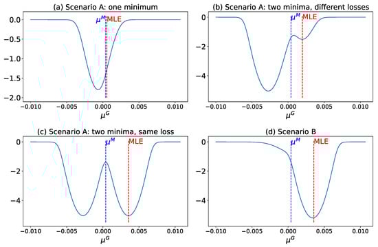
Figure 1.
Loss functions of the classical oracle GA estimator in different scenarios.
Despite having access to , the loss function of the classical oracle GA estimator can sometimes produce estimates worse than those of the MLE. In Figure 1a, the classical oracle GA estimator deviates significantly from the true mean, offering no advantage over the MLE, even when the true mean is explicitly known.
Figure 1b,c illustrate cases where the loss function defined in Equation (12) exhibits multiple minima. In particular, non-convexity in the loss function poses significant challenges for optimization, such as convergence to local minima or divergence to infinity. The severity of these issues depends on the degree of non-convexity and may be partially addressed through methods like random restarts. Nevertheless, these complications increase the computational effort required to obtain reliable estimates. Moreover, as seen in Figure 1a, even when the global minimum is successfully located—as in Figure 1b—it may still be farther from the true mean than the maximum likelihood estimator (MLE), raising concerns about the statistical efficiency of the classical oracle GA estimator.
Additionally, for certain combinations of and , the loss function may have multiple global minima, as depicted in Figure 1c. In such cases, the classical oracle GA estimator admits more than one equally optimal solution, each yielding the same loss value. This inherent ambiguity cannot be resolved through numerical optimization techniques alone and may lead to confusion, inconsistent interpretations, or suboptimal decisions, ultimately compromising the robustness of the estimation process.
The loss function demonstrates more favorable properties in Scenario B. As shown in Figure 1d, it consistently exhibits a single minimum. Moreover, this minimum is between the true mean and the MLE, as established in Proposition 4. Consequently, in Scenario B, the classical oracle GA estimator is always closer to the true mean than the MLE, highlighting its improved accuracy and robustness in this setting.
4.2. Classical Family-Oracle GA Estimator
Following the methodology of the previous section, we analyze the loss function of the classical family-oracle GA estimator. Figure 2a presents a visualization analogous to Figure 1a, demonstrating that the GA estimator can, in some instances, perform worse than the MLE by deviating further from the true mean. In this figure, the point represents the estimates produced by the classical family-oracle GA estimator where . The point denotes the true mean, while represents the MLE for the true data and generator, i.e., and . It is evident that lies farther from than , indicating that, in certain samples, the classical GA estimator may yield less accurate estimates than the MLE.
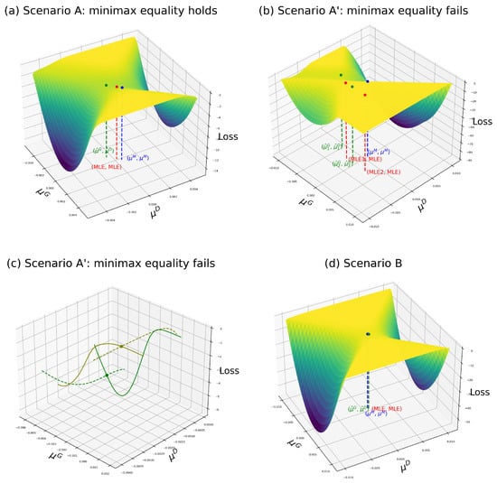
Figure 2.
Loss functions of the classical family-oracle GA estimator in different scenarios.
In contrast, the case illustrated in Figure 1b and Figure 2b provides an example in which the min–max optimization procedure fails due to the loss function not being convex–concave over the plane. Consequently, no saddle point exists, and the minimax equality does not hold:
The min–max solution is denoted as , with its corresponding MLE labeled (MLE1, MLE), while the max–min solution is , with corresponding MLE tag (MLE2, MLE).
The absence of a saddle point in this setting presents a practical challenge; multiple suboptimal solutions may emerge across simulation runs, undermining estimator reliability. Figure 2c shows the behavior of the loss function near these two points. The dashed green line represents the loss function with held constant, while the solid green line represents the loss with fixed. Similarly, the dashed olive line fixes , and the solid olive line fixes . These plots reveal that neither nor corresponds to a local maximum with respect to or a local minimum with respect to . As a result, the classical family-oracle GA estimator fails to reach an optimal solution in this scenario, degrading its performance.
Finally, Figure 2d illustrates the loss function of the classical family-oracle GA estimator in Scenario B. As expected, the loss function exhibits convex–concave behavior, and a unique saddle point is identified. Moreover, the resulting estimator is notably closer to the MLE, where the red and the green dot are the same, indicating improved performance.
4.3. Alternative GA Estimator
The loss functions of the alternative GA estimator are illustrated in Figure 3. In contrast, Figure 1a, Figure 2a, and Figure 3a show that the alternative GA estimate no longer deviates from the MLE. Instead, discrepancies arise only in , attributable to random noise from the generator. Consequently, the alternative GA estimator closely approximates the MLE and outperforms the classical oracle GA estimator with the family-oracle discriminator.
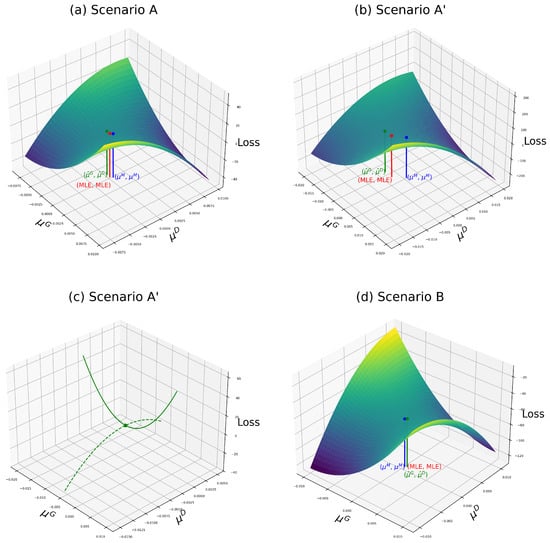
Figure 3.
Loss functions of the alternative GA estimator in different scenarios.
Moreover, the issue of the non-existence of a saddle point—observed with the classical family-oracle GA estimator—is resolved in the alternative GA framework. Figure 3b depicts a well-behaved convex–concave loss function exhibiting a unique saddle point that serves as a local minimum with respect to and a local maximum with respect to . This property is further clarified in Figure 3c, where the solid green line represents the loss function with fixed, and the dashed green line represents the function with fixed.
4.4. Distribution of Estimators
In the previous sections, we have produced five GA estimators. These are the classical GA with the discriminator’s estimator for the generator (see Equation (14)), the classical GA with the family-oracle discriminator’s estimators for the discriminant and generator (see Equation (16)), and the alternative GA method’s estimators for the discriminant and generator (see Equations (17) and (18)). To compare the statistical properties of these five GA estimators with the MLE, we construct density plots for all.
Specifically, we generate 20,000 simulated samples of and , where represents the trial index. For each trial n, the five estimators are computed based on the corresponding and . The resulting distributions of the estimators are visualized using Gaussian kernel density estimates based on histograms from the 20,000 trials. These density plots are presented in Figure 4 and Figure 5.
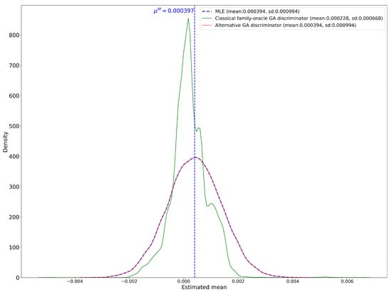
Figure 4.
Density of estimator for using the classical GA method and the alternative GA method with the family-oracle discriminator.
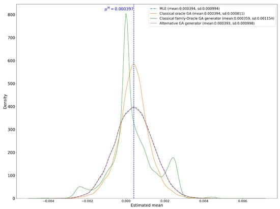
Figure 5.
Density of estimators for using the classical GA method, the oracle and the family-oracle, and the alternative GA method and the MLE.
Figure 4 is about the estimators of . It presents three distributions: the distributions of the estimators for the discriminator () from both the classical GA method with the family-oracle and the alternative GA method with the family-oracle. It also includes the distribution of the MLE, while the true mean is indicated by the dashed blue vertical line. The density plots for the alternative GA method and MLE are all symmetric around the true mean. Notably, the density plot of the alternative GA method closely resembles that of the MLE. Descriptive statistics support these observations. The means and standard deviations of the alternative GA method and the MLE are nearly identical, confirming the strong performance of the alternative GA method.
In contrast, the classical GA method with the family-oracle discriminator exhibits a significant bias relative to the other estimators, despite having the lowest standard deviation (0.000668). To see the implication of this low standard deviation, we compute confidence intervals for these parameters, under the classical assumption of a Gaussian distribution for the estimators. At the 1% significance level, the 99% confidence interval for the mean of the classical family-oracle GA discriminator is , which excludes the true mean—indicating substantial bias and limited reliability for estimating the true value. On the other hand, the 99% confidence intervals for both the MLE and the alternative GA method are , and, for the classical oracle GA estimator, ; all of these intervals contain the true mean. The bias seems to arise from the possibility that no saddle point exists for certain sample paths, and , as discussed in Section 4.3. The failure of the min–max optimization in these cases highlights the instability of the classical GA method with the family-oracle discriminator and suggests challenges in applying this method reliably in financial practice.
Figure 5 targets the estimators of . It displays distributions of four estimators for the generator (). These are the distribution from both the classical GA method with the family-oracle and with the oracle discriminator and the alternative GA method with the family-oracle. It also includes the true parameter () and the distribution of the corresponding MLE.
In this figure, the distribution of the estimator from the classical GA method with the family-oracle discriminator deteriorates significantly, exhibiting a multi-modal pattern. Although its mean (0.000359) is closer to the true mean than in Figure 4, the estimator remains substantially biased, and its standard deviation increases to 0.001154. Moreover, the 99% confidence interval for the mean is , which excludes the true mean, indicating persistent bias.
The estimator from the alternative GA method also shows a slight decline in performance. Its mean decreases marginally from 0.000394 to 0.000393, and its standard deviation increases from 0.000994 to 0.000998. However, these changes are minimal and can be attributed to the inherent randomness in the generator. Its 99% confidence interval for the mean remains robust at .
Lastly, the estimator from the classical GA method with the oracle discriminator shows great performance, exhibiting the same mean and a smaller standard deviation (0.000811) compared to the other estimators. However, this improved performance is expected, as the classical GA method with the oracle discriminator incorporates the true mean into its loss function, effectively giving it an unfair and unrealistic advantage.
Overall, this figure reinforces that the classical GA estimator with the family-oracle discriminator is largely unreliable, whereas the alternative GA estimator remains statistically sound and robust.
5. Conclusions
Summarizing our methodology and main findings, using a simple setting of a Gaussian i.i.d. sequence with an unknown mean, we reveal several pitfalls for the classical GA methodology of [1] in finite samples. Our intention with this simple setting is, on the one hand, to gain a deeper understanding of the GA methodology by relying on a control experiment, i.e., where the true data generator or model is known. On the other hand, we intend to make the case that, if the methodology falters in simple settings, then it should be of concern, and further studies should be carried out in more complex settings.
In order to favor the methodology further, avoiding approximations to the discriminant or generator, we assume that the discriminants and generators are in the same family as the true data-generating process (family-oracle). We also try the oracle discriminant case but not as a serious contender due to its impracticality. In other words, the discriminant is perfect as it knows the true model. Theoretically and numerically, we find that the classical GA method might deliver multiple local optima, or even multiple global optimal in the oracle case, while occasionally failing to deliver a saddle point in the family-oracle setting. Moreover, the estimator implied in the family-oracle is biased with smaller variance than the maximum likelihood estimator. Such a combination of bias and small variance would only keep practitioners away from the true model.
Given the limitations of the classical GA method, we propose an alternative GA method that delivers, theoretically, a unique saddle point. This optimal point, as an estimator, is unbiased and consistent. Moreover, numerically, the methodology is very stable and a little time-consuming. The findings in the numerical sections were tested for robustness, with many other examples excluded from the paper to streamline the presentation.
In future research, the ideas presented in this paper will be used as a blueprint to study more advanced models (i.e., true data-generating processes) like non-Gaussian i.i.d series, autoregressive models, or autoregressive conditional heteroskedasticity (ARCH) models, as well as other GA methodologies or loss functions like Geometric GA, Least-Squares GA, and Wasserstein GA methods. And, more importantly, the analyses should be extended, first to a discriminant or generators relying on neural networks (NN), as a way of testing the capacity of NNs to uniquely and reliably capture true models, and, secondly, to true data-generating processes that are NNs themselves. If NN discriminators and generators can capture these models in control experiments, then they have a real shot at capturing reality; otherwise, the hype around NNs might be an illusion.
Author Contributions
Methodology, M.E.-A. and Y.J.; software, Y.J.; validation, M.E.-A. and Y.J.; formal analysis, M.E.-A. and Y.J.; investigation, M.E.-A. and Y.J.; data curation, M.E.-A. and Y.J.; writing—original draft, M.E.-A. and Y.J.; writing—review and editing, M.E.-A. and Y.J.; visualization, Y.J. All authors have read and agreed to the published version of the manuscript.
Funding
This research received no external funding.
Data Availability Statement
Data will be made available upon request.
Conflicts of Interest
The authors declare no conflicts of interest.
Appendix A. Nomenclature and Proofs
Appendix A.1. Nomenclature
The following table describes the symbols, and their interpretation, used throughout the paper.

Table A1.
Nomenclature.
Table A1.
Nomenclature.
| Symbols | Comment |
|---|---|
| Number of samples, size of each sample | |
| Number of generated samples, size of each sample | |
| Mean of Gaussian r.v., true model | |
| Variance of Gaussian r.v., true model | |
| D | Discriminator, |
| , | Parameter of discriminator, estimator |
| , | Parameter of generator, estimator |
| Sample i generated of size | |
| Sample of size T from true model | |
| L | Generic loss function asymptotic |
| Generic loss function finite sample | |
| Classical GA, loss function asymptotic | |
| Classical GA, loss function finite sample | |
| Alternative GA, loss function asymptotic | |
| Alternative GA, loss function finite sample |
Appendix A.2. Proofs
Lemma A1.
Let , , and . Then, .
Proof.
We begin by proving that . Defining and expressing the expectation in integral form, we obtain
Focusing on the second integral,
Here, the third line follows from Tonelli’s theorem, and the final inequality holds due to the assumption that . A similar argument establishes that the first integral is also finite, thereby confirming that .
Since this expectation is finite, we can apply Fubini’s theorem:
Thus, we have established the desired result. □
Proof.
Proof of Proposition 1.
First, recall that the oracle discriminator can be written as
We then search for the best generator, i.e., the best :
The result is shown next:
The first-order condition is
or
Applying Lemma A1 to the FOC, , and the FOC is
Since , the FOC requires
Since for all x, , and the FOC is satisfied only when . Now, we prove that the unique extreme of the classical GA problem is . Next, we prove that is a minimum.
The second-order derivative of the loss function with respect to is
where . At , the second-order derivative equals
Proof.
Proof of Proposition 2. First, we produce the first-order condition (FOC) with respect to .
The FOC reads
where the integrations are in dimensions T and , respectively.
It is easy to see that, if , then the FOC becomes
and satisfies this FOC regardless of .
Next, we produce the first-order condition (FOC) with respect to :
The FOC reads
Hence, the FOC(s) would be
It is easy to see that the point satisfies the FOC(s).
Note that, with , the optimal discriminator would be the oracle.
□
Proof.
Proof of Proposition 3. For convenience, we work with T and K rather than and . Recall,
This is the likelihood of a Gaussian model with mean and volatility .
The new objective function is
with . Then, we have
and
Together, the loss function becomes
Let us compute the first-order condition with respect to :
Now, we compute the first-order condition with respect to :
The first-order conditions are satisfied uniquely if the following relation holds:
A sufficient condition for a saddle point is a negative Hessian.
Finally, the Hessian is
Therefore, the point is the unique saddle point for the given optimization problem if and . Moreover, if , then , making the critical point a maximum in . □
Proof.
Proof of Proposition 4.
For convenience, we work with K rather than . Let us compute the first-order condition with respect to :
We have
then
and
Together,
Hence, we obtain a highly non-linear equation for , where we should recall that , and
Let us define
Then, we can write the first-order condition as follows:
An implicit solution could be written as
Note that is very close to a solution of the FOC when , , and T is sufficiently large.
For the case of , we compute the first-order condition with respect to on the objective function:
Together, we obtain
Let us continue simplifying the FOC:
Applying Lemma A1,
As a result, unless . Also, , the MLE, unless . When , the unique minimum is .
Furthermore, since and , we find that one of the following is true: (i) ; (ii) ; or (iii) . Thus, the infinite-sample classical oracle GA estimator is between the true mean and the MLE . □
Proof.
Proof of Proposition 5.
Recall that we have
Let us compute the first-order condition with respect to :
Then,
and
Together,
Hence, we obtain a highly non-linear equation for , where we should recall that , and .
Next, we compute the first-order condition with respect to :
then
and
Together,
We also obtain a highly non-linear equation for .
Let us denote
Then, we can write the first-order conditions as follows:
which can be simplified to
For the case , we first compute the first-order condition with respect to on the objective function:
where , and we obtain
Together, we obtain the FOC:
Now, we compute the first-order condition with respect to :
Together, we obtain
Then, the system of the FOC(s) is as follows:
□
Proof.
Proof of Proposition 6.
For convenience, we work with T and K rather than and . Let us compute the first-order condition with respect to :
We have
and
Together,
Hence, we obtain the following equation, where we have used :
Now, we compute the first-order condition with respect to :
As before,
and
Together,
leading to the second equation:
The estimates proposed by our GAN would be the system of two equations:
which leads to
We need to show that the solution to the FOC is unique, and it constitutes a saddle point.
Let us compute the Hessian:
Finally, the Hessian is, for and ,
The point is the unique saddle point for the given optimization problem, and a maximum in , if .
It can be seen that unbiasedness and consistency follow by noticing that
and
both approach zero as T, and K goes to infinity. □
References
- Goodfellow, I.; Pouget-Abadie, J.; Mirza, M.; Xu, B.; Warde-Farley, D.; Ozair, S.; Courville, A.; Bengio, Y. Generative adversarial networks. Commun. ACM 2020, 63, 139–144. [Google Scholar] [CrossRef]
- Wiese, M.; Knobloch, R.; Korn, R.; Kretschmer, P. Quant GANs: Deep generation of financial time series. Quant. Financ. 2020, 20, 1419–1440. [Google Scholar] [CrossRef]
- Takahashi, S.; Chen, Y.; Tanaka-Ishii, K. Modeling financial time-series with generative adversarial networks. Phys. A Stat. Mech. Its Appl. 2019, 527, 121261. [Google Scholar] [CrossRef]
- Yang, J.; Gong, X.; Fang, A. Extreme Risk Spillover from Commodity Markets to Green Finance Markets: New Evidence Utilizing GAN and GARCH Model. Comput. Econ. 2025, 1–29. [Google Scholar] [CrossRef]
- Ganguly, S. Implementing quantum generative adversarial network (qgan) and qcbm in finance. arXiv 2023, arXiv:2308.08448. [Google Scholar] [CrossRef]
- Liao, S.; Ni, H.; Sabate-Vidales, M.; Szpruch, L.; Wiese, M.; Xiao, B. Sig-Wasserstein GANs for conditional time series generation. Math. Financ. 2024, 34, 622–670. [Google Scholar] [CrossRef]
- Eckerli, F.; Osterrieder, J. Generative adversarial networks in finance: An overview. arXiv 2021, arXiv:2106.06364. [Google Scholar] [CrossRef]
- Kaji, T.; Manresa, E.; Pouliot, G. An adversarial approach to structural estimation. Econometrica 2023, 91, 2041–2063. [Google Scholar] [CrossRef]
- Lim, J.H.; Ye, J.C. Geometric GAN. arXiv 2017, arXiv:1705.02894, 02894. [Google Scholar] [CrossRef]
- Mao, X.; Li, Q.; Xie, H.; Lau, R.Y.; Wang, Z.; Smolley, S.P. Least Squares Generative Adversarial Networks. In Proceedings of the 2017 IEEE International Conference on Computer Vision (ICCV), Venice, Italy, 22–29 October 2017; pp. 2813–2821. [Google Scholar] [CrossRef]
- Arjovsky, M.; Chintala, S.; Bottou, L. Wasserstein generative adversarial networks. In Proceedings of the International Conference on Machine Learning, Sydney, Australia, 6–11 August 2017; pp. 214–223. [Google Scholar]
- Athey, S.; Imbens, G.W.; Metzger, J.; Munro, E. Using wasserstein generative adversarial networks for the design of monte carlo simulations. J. Econom. 2021, 240, 105076. [Google Scholar] [CrossRef]
- Kaji, T.; Manresa, E.; Pouliot, G.A. Adversarial Inference Is Efficient; AEA Papers and Proceedings; American Economic Association: Nashville, TN, USA, 2021; Volume 111, pp. 621–625. [Google Scholar]
- Farnia, F.; Wang, W.W.; Das, S.; Jadbabaie, A. Gat–gmm: Generative adversarial training for gaussian mixture models. SIAM J. Math. Data Sci. 2023, 5, 122–146. [Google Scholar] [CrossRef]
- Chakraborty, S.; Bartlett, P.L. On the statistical properties of generative adversarial models for low intrinsic data dimension. arXiv 2024, arXiv:2401.15801. [Google Scholar] [CrossRef]
- Birrell, J. Statistical Error Bounds for GANs with Nonlinear Objective Functionals. arXiv 2024, arXiv:2406.16834. [Google Scholar]
- Barron, E.N. Game Theory: An Introduction; John Wiley & Sons: Hoboken, NJ, USA, 2024. [Google Scholar]
- Boyd, S.; Vandenberghe, L. Convex Optimization; Cambridge University Press: Cambridge, UK, 2004. [Google Scholar]
- Piessens, R.; de Doncker-Kapenga, E.; Überhuber, C.W.; Kahaner, D.K. Quadpack: A Subroutine Package for Automatic Integration; Springer: Berlin/Heidelberg, Germany, 1983; Volume 1. [Google Scholar]
Disclaimer/Publisher’s Note: The statements, opinions and data contained in all publications are solely those of the individual author(s) and contributor(s) and not of MDPI and/or the editor(s). MDPI and/or the editor(s) disclaim responsibility for any injury to people or property resulting from any ideas, methods, instructions or products referred to in the content. |
© 2025 by the authors. Licensee MDPI, Basel, Switzerland. This article is an open access article distributed under the terms and conditions of the Creative Commons Attribution (CC BY) license (https://creativecommons.org/licenses/by/4.0/).