Abstract
Counting and density estimation of cone cells using adaptive optics (AO) imaging plays an important role in the clinical management of retinal diseases. A novel deep learning approach for the cone counting task with minimal manual labeling of cone cells in AO images is described in this paper. We propose a hybrid multi-task semi-supervised learning (MTSSL) framework that simultaneously trains on unlabeled and labeled data. On the unlabeled images, the model learns structural and relational features by employing two self-supervised pretext tasks—image inpainting (IP) and learning-to-rank (L2R). At the same time, it leverages a small set of labeled examples to supervise a density estimation head for cone counting. By jointly minimizing the image reconstruction loss, the ranking loss, and the supervised density-map loss, our approach harnesses the rich information in unlabeled data to learn feature representations and directly incorporates ground-truth annotations to guide accurate density prediction and counts. Experiments were conducted on a dataset of AO images of 120 subjects captured using a device with a retinal camera (rtx1) with a wide field-of-view. MTSSL gains strengths from hybrid self-supervised pretext tasks of generative and predictive pretraining that aid in learning global and local context required for counting cones. The results show that the proposed MTSSL approach significantly outperforms the individual self-supervised pipelines with an RMSE score improved by a factor of 2 for cone counting.
1. Introduction
Medical imaging of the photoreceptors and microstructures of the human retina using adaptive optics (AO) technology holds great promise for managing eye diseases. Several eye diseases including Stargardt disease, Retinitis Pigmentosa, Inherited Retinal Disease, and Autoimmune Retinopathy, reduce the density of cone cells, resulting in loss of color vision and spatial visual acuity [1,2,3,4,5,6]. The AO imaging technology provides practitioners with an alternative way to manage diseases by visualizing and analyzing cone cell densities across the retina without resorting to histological sampling [7,8,9,10,11,12,13]. Devising approaches that can accurately count cones and their densities across the retina is important to realize the benefits of the AO technology and manage diseases to prevent visual impairments.
Several deep machine learning (ML) approaches have been explored to measure cone densities in AO images [4,14,15,16,17,18]. These works use a supervised learning approach using carefully curated datasets such as [19] where cone cells in each image have to be manually annotated by experts. Moreover, careful curation limits from generalizing the approach to different regions. The large data volume required for these approaches requires experts to annotate individual cone cells in many images. Annotating cells in a few images is insufficient since spatial cone distributions and their densities at different regions of interest (ROIs) (sample ROI shown in Figure 1 across the retina may be of clinical significance). Further, some of the newer AO devices based on retinal cameras, allowing a wider field-of-view in comparison to the AO Scanning Laser Ophthalmoscope (SLO) [20,21], produce relatively lower resolution images, which makes manual annotation more error-prone. The accuracy of the automatic cone annotation provided by some of these devices needs improvement to be used reliably. Low-resolution AO images and variable ROI sizes compound the challenge of learning effective representations from limited labeled data. Recent work has applied deep learning, specifically multi-task architectures, to jointly localize the fovea and learn discriminative features despite the small size of the dataset and low resolution of the AO images [22]. Self-supervised learning (SSL) techniques have shown immense success in various domains including medical domains for utilizing unlabeled data to extract features from the dataset while using a few annotated data, drastically reducing the annotation efforts and improving feature learning abilities [23,24].
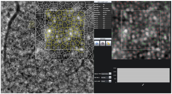
Figure 1.
Snapshot of AODetect software automatic (red) and manual (green) annotations for the selected ROI shown on the left.
In this paper, we propose a semi-supervised learning framework tailored for counting cones and estimating their densities in AO images produced using retinal camera devices. Popularly employed self-supervised learning (SSL) techniques have shown great success. The SSL approaches use pretext tasks to augment unlabeled data and produce a pretrained model, which is then finetuned using limited amounts of labeled data to perform the downstream task. However, the two-stage strategy might cause the pretrained model to deviate from the downstream task and require resources for both pretraining and finetuning. Additionally, state-of-the-art augmentation-based SSL techniques, such as contrastive or non-contrastive SSL, are observed to be insufficient for AO images as the augmentations do not introduce adequate diversity or variations. Consequently, this limits the ability of these pretrained models to learn robust and generalizable features. Instead of relying solely on augmentation-based SSL and a two-stage pretraining and finetuning strategy, our method jointly optimizes two self-supervised pretext tasks on unlabeled images while simultaneously supervising a density-map estimation head on a small set of annotated images. SSL approaches have been used earlier for crowd counting, harvest or crop counting, and multi-object counting [25,26,27]. The earlier SSL approaches have commonly used rotation and L2R as pretext tasks for counting [26,27]. This article is a revised and expanded version of a paper [28] entitled “COINS: Counting Cones Using Inpainting Based Self-supervised Learning”, which was presented at the 46th Annual International Conference of the IEEE Engineering in Medicine and Biology Society (EMBC); Orlando, FL, USA; 15–19 July 2025.
The proposed semi-supervised framework employs two hybrid self-supervised pretext tasks—inpainting (IP) and learning-to-rank (L2R) on unlabeled AO images together with a supervised density estimation task on a small set of labeled images. The IP task forces the network to model local structural patterns of cone morphology, and the ranking task instills a global ordering bias of which image contains more cones. IP, a popular pretext task, is especially well-suited for cone counting since it allows for the incorporation of context information in pretrained models, which has been attributed to improving counting accuracy in supervised learning models [25,29]. Unlike natural images, which capture a wide range of colors and textures that aid deep learning models in discriminating the features, applying similar models to medical images, which are often gray-scale or have less variations, is challenging. Medical tasks frequently require detecting subtle variations to distinguish anomalies or background from the foreground [30]. In AO images, differentiating cones from the background and blurry regions is especially difficult due to their small size and minimal contrast. Adopting techniques like generative SSL, which learn local features at the pixel level, proves particularly beneficial in such scenarios [30]. Moreover, learning context information is crucial when the objects are small, given their dense distribution [31]. IP provides the context that helps the model to learn the spacing, local contrast, geometry, and subtle variations from the background required to identify the cones.
In the IP pretext task, regions in the images are initially masked and a model is learned to reconstruct the masked region given the context information provided by the rest of the image, typically used for classification and segmentation tasks. The distribution of cones varies in different regions of the eye. By ranking the patches, the models learns natural ordering to assess relative density without requiring actual counts. This could also be of direct clinical relevance to understand the change in densities of different regions without actual count estimation. This relative judgment learned by the model provides strong cues towards identifying subtle density variations and aids in the count estimation task. Capitalizing on the potential benefits of these strategies and their relevance for AO images, where grasping the global and local context is crucial for understanding the distribution and features of cones, we propose to utilize IP pretext along with L2R in our approach.
Our results show that the proposed MTSSL approach considerably improves the cone counting performance by reducing the count error by a factor of ≈2 compared to the individual self-supervised learning tasks.
2. Methodology
The proposed multi-task SSL approach comprises three branches, including IP and L2R as auxiliary tasks that use unlabeled data and density estimation as the main task on labeled images. The overall flow of the approach is shown in Figure 2. In the following sections, we first present each pretext task as a standalone SSL method with pretraining and finetuning for counting as a downstream task. Then, we introduce our MTSSL framework, which combines both pretext objectives alongside supervised density estimation.
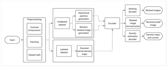
Figure 2.
Overall flow of approach.
2.1. Inpainting SSL
The IP pretext task learns features from unlabeled images by learning to reconstruct missing regions in an image. Some regions of the images are removed in IP to create a masked image, and a model is learned to fill these regions as close to the original image as possible [32]. The pretrained models learn the global context features and spatial arrangement of objects while reconstructing the image. Learning the context information is essential and has been noted in other counting tasks [25]. For performing IP, context-encoders and Generative Adversarial Networks (GANs) have been popularly employed to construct models. Besides effectively learning the spatial arrangement through inpainting, GANs are efficient in pixel generation, thereby understanding the structural components of the images [33]. These capabilities align seamlessly with the objectives of learning cone distributions and structures, crucial for accurate cone counting. By leveraging these capabilities to comprehend the spatial arrangement and structure of cones, IP emerges as a well-suited SSL pretext task for acquiring representations conducive to cone counting and densities in AO images. Therefore, we utilize GAN-based IP as a pretext task to learn features for cone counting, generative SSL.
2.2. Learning-to-Rank SSL
The L2R [26] has been used for counting objects other than cone cells. The L2R learns representations by generating, from each unlabeled image, N concentric image patches all centered around a point on the image. Each patch in the concentric set of patches is larger than the immediately nested one by a predefined scale factor. Each of these patches gets a rank that progressively increases as we move from the inner patches to the outer ones. These ranks are learned such that the innermost nested patch has the lowest rank whereas the outermost patch has the highest rank. All patches are resized to the original image size and these ranked images are input to the L2R model. The model learns representations by learning the rank of each patch in the set of patches of the image.
2.3. Downstream Cone Counting
The downstream task involves finetuning the pretrained model for cone counting with few annotated cone images. Traditional counting techniques often follow two main approaches [34]. The first approach performs object detection, which is then followed by counting the detected objects to obtain the count of objects of interest. In the second approach, regression-based methods are used to obtain the count of objects of interest directly. While the former approach provides the spatial distribution of the objects in an image by providing localization information, this approach, especially when the objects of interest are large in number, is computationally expensive. The regression-based approach lacks localization information and merely provides an overall count of objects of interest in an image.
In order to address these limitations, density estimation has grown widely popular and provides both counts of objects of interest along with localization information through density-map prediction [34]. We adopt a density estimation-based method for the downstream task of cone counting, which shows the distribution of cones within the image. The downstream task of cone counting. The task involves finetuning the pretrained model with a few annotated cone images. These images are labeled using dot annotations, where each dot represents the location of the cone in the AO image patches. The annotation was performed by experts, where the preliminary pseudo-annotations were obtained using the DT algorithm by adjusting the parameters for patches of different sizes. The experts further made adjustments to annotate missing cone labels and rectify any incorrect labels. In this study, two dedicated annotators were assigned to review and correct these labels by providing a clear correction protocol. To guard against overlooked errors, they were supervised by a peer who spot-checked a random 10% subset, and any discrepancies were resolved by joint review. This consensus-driven process, with three annotators and a clear correction protocol, ensured a high level of annotation consistency. These dot maps are transformed into density maps by applying a Gaussian filter as ground truth (GT).
2.4. Multi-Task Semi-Supervised Learning
Multi-task learning has been shown to improve feature representation learning, thereby improving the generalization abilities of a model [35,36]. Multi-task learning strategies have been employed in situations when a smaller amount of labeled data is available to learn more features pertaining to different tasks, including counting [37,38]. This technique typically employs a shared encoder with task-specific decoders. Multi-task self-supervised pretraining, and multi-task semi-supervised learning strategies have been studied and shown to not only exhibit better generalization abilities [39] but it was also observed that semi-supervised methods achieve accuracies similar to self-supervised and fully supervised methods with significantly less data [40,41,42,43]. Self-supervised techniques, though, can learn generalizable features, might deviate from the target downstream task, and require finetuning to adapt to the target task. Frozen pretrained models might not be sufficient for the downstream task. Semi-supervised techniques overcome this by jointly training with unlabeled and labeled data, where unlabeled data can be used to introduce the inductive bias, and joint optimization using the mixed loss of auxiliary task with the main task helps to learn task-specific features [39].
The proposed approach blends the advantages of both L2R and IP methods as a semi-supervised multi-task strategy, a hybrid of both predictive and generative pretraining techniques combined with density estimation supervision to learn features from cone images for counting. Hybrid SSL pretraining techniques have been employed in the medical domain [31,44]. While conventional semi-supervised multi-task learning typically involves multiple supervised tasks defined over labeled data, our approach introduces a novel formulation where multiple self-supervised pretext tasks are employed. The architecture is shown in Figure 3.
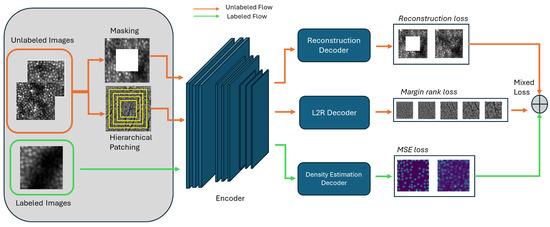
Figure 3.
The proposed MTSSL architecture.
2.5. Point Map Generation
Following the density map and count estimation, we perform post-processing to obtain a point map from the density maps to accurately locate the cones. Localization of objects from density maps is well-known as a non-trivial problem. We employed two methods to perform localization. First, by computing peak local maximum, these peaks provide the centers of the estimated blobs in density maps and thereby the centers of cones. The second method used was from [45], which uses the Sinkhorn distance minimization strategy to generate the point map from density maps.
3. Experiment Setup
To evaluate the effectiveness of our proposed MTSSL framework, we conducted a series of experiments designed to assess both individual and combined contributions of the pretext tasks. The experiments are organized as follows:
- Single-Task Self-Supervised Learning (STSSL)—We first evaluated each pretext task—IP and L2R individually. Each model was pretrained using only the respective self-supervised objective on unlabeled images, and subsequently finetuned using the labeled images for the downstream cone counting task via supervised density-map regression.
- Multi-Task Self-Supervised Pretraining + FineTuning (MTSSP)—Next, we jointly pretrained the model using both IP and L2R pretext tasks on unlabeled data. The frozen shared encoder was then combined with a decoder finetuned on labeled data for cone counting.
- Proposed MTSSL—Finally, we evaluated our proposed approach, where IP, L2R, and density-map supervision were jointly optimized in a single training loop.
The following sections provide details on the dataset and the above-mentioned experiments.
3.1. Dataset
The images used in the study were captured from 120 healthy subjects with an AO rtx1 device following Helsinki declaration guidelines. The retinas of these subjects were undilated. For each subject, five regions, all with an eccentricity of × (1162 m), were captured with the centers at (0, 0), (0, −2), (0, +2), (2N, 0), and (2T, 0) producing a total of 600 images across 120 subjects. These regions have about overlap. The AO rtx1 device captured 40 images in a span of 4 s at each of these 5 regions and processed these 40 images to generate an averaged final image for each region using a cross-correlation registration method [46]. The AOdetect 3.0 image acquisition recognition software (Imagine Eyes; Orsay, Paris, France) was used to select regions of interest (ROI) within the × field of × (93 m) in each of these averaged final images and provided automatic identification of cones in this ROI.
The AOdetect software employs a Delauney Triangulation (DT)-based approach to perform the automatic cone detection [46]. A sample final image along with manual and automatic cone detection of the selected ROI is shown in Figure 1. The image on the left also highlights the Voronoi diagram of the selected ROI. The software also allows manual adjustment of the markings of the automatically detected cones within the ROI [46]. During image capturing, events like eye blinking of the participants cause artifacts in the images, resulting in noisy and blurred images. Thirty such images are unmeasurable and were removed from the dataset, resulting in a total of 570 usable images. The wide field-of-view of rtx1 devices in comparison to AOSLO devices results in lower resolution of the images. Contrast adjustment was performed on the images as a preprocessing step to enhance the cones’ visibility in the images. All the images are patched to be used for both pretraining and downstream tasks to improve the identification of cones and increase the volume of the dataset.
The dataset with 570 images was further filtered to exclude the center images as these images have an overlap with the other four regions in order to eliminate any redundancy caused by patching. Also, a few images that had more blurry regions were removed, resulting in 440 images. Contrast enhancement was performed. These images were patched for the experiments with a patch size of 150 × 150. Of the 440, 50 images were randomly selected for testing purposes. The total patches thus generated were about 47,000, which were subsequently split for pretraining and downstream tasks.
3.2. STSSL—IP
For the IP STSSL, the GAN architecture followed [33] with modifications to the generator. The generator was modified with a VGG16 encoder as a baseline following [47] to be consistent with the rest of the experiments. The model comprises ten convolution layers and a decoder with five deconvolution layers, both equipped with leaky ReLU activations and batch normalization. The decoder outputs the reconstructed masked parts, the same size as the masked parts cropped out of the original image. Meanwhile, the discriminator uses five convolution layers with ReLU activations. For the generator, the loss function is a combination of mean squared error (MSE) loss, aimed at minimizing adversarial loss between the discriminator and generator, and pixel-wise loss computed using L1 loss to minimize the distance between generated and original pixels. The loss is provided in (1) where is set to 0.2.
For the IP task, the random masking was performed with a single 64 × 64 patch. The GAN architecture was trained for 150 epochs, and based on the reconstruction error, the best model was selected to transfer to the downstream task. Adam optimizer was utilized with a learning rate set to . For the generative loss, alpha was experimentally set to 0.2. The discriminator loss used the MSE loss of the real vs. masked parts and the generated vs. fake patches. The batch size was set to 128. The downstream was performed using approximately 4800 images, which were split into training and validation sets with a split ratio of 0.2 for validation, and were trained for 50 epochs. Adam optimizer had a learning rate set to . The combined loss of MSE and dice loss was used with a weight of 0.4 for dice loss.
3.3. STSSL—L2R
In the L2R method, 5 patches were generated for each image to learn to rank. In this study, the anchor is always set as the center of an image (see the concentric yellow square patches in Figure 4). These patches are input to the L2R model and the resulting feature maps are ranked using margin ranking loss (see (2)) to learn the ranking.
where is the densities of feature maps from smaller regions and is the densities of feature maps from the super-region, hence when < , which is the correct ranking, the loss returns zero, otherwise it propagates the loss towards learning the appropriate ranking of the patches.
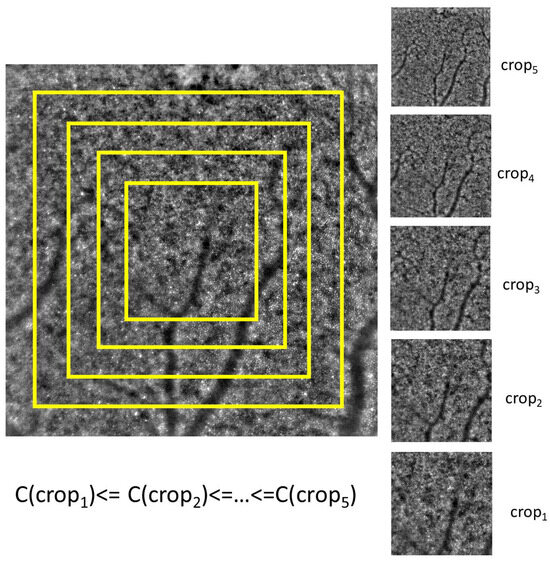
Figure 4.
Crops generated for performing L2R.
The architecture of L2R uses VGG16 as a baseline encoder for efficient feature extraction as proposed in [47], same as the generator encoder of the IP task. The decoder comprises six upsampling layers generating the feature maps of the same size for all patches to rank them using ranking loss.
Pretraining was performed for 100 epochs, with Adam optimizer, learning rate of . Margin ranking loss was used for pretraining. The downstream task was trained for 50 epochs with MSE loss, Adam optimizer, and learning rate . The pretraining and finetuning splits were the same as those used in the IP approach. The loss function for the L2R method was also the same as IP.
3.4. MTSSP
The MTSSP was performed for 150 epochs with the other parameters the same as mentioned above, and downstream for 50 epochs. The loss for MTSSP is the combination of and . However, the GAN architecture was replaced with only a reconstruction encoder–decoder instead of using a discriminator to reduce the model complexity. Hence the of was set to 0 in this case (see (3) below). The hypermeters and were set to 0.5 for a tradeoff between the tasks:
3.5. Downstream
From the IP pretext task, the pretrained generator encoder was transferred to train on the labeled dataset. Similarly, the encoder of the L2R and the shared encoder of MTSSP pretrained models were used for downstream. The density decoder comprises six convolution transpose layers to generate density maps the same size as the input image. For finetuning, all three methods use a combination of mean squared error (MSE), which minimizes the GT and predicted counts, and dice loss, which aids in generating sharp density maps as a loss function (see (4) below). was set to 0.4. The counts from predicted maps are produced by integrating the density maps. We performed K-fold cross-validation, 5-fold, with shuffling to ensure a randomized split of the labeled data into training and test sets.
3.6. MTSSL
The approach employs the same encoder as mentioned in the above methods, which is shared for all the tasks, and a task-specific decoder for each task. A mixed weighted loss (see (5)) is implemented, comprising pixel-wise loss for reconstruction, marginal-ranking loss for L2R, and MSE loss. In the MTSSL, the discriminator for the IP task is removed to reduce the complexity, and hence here is loss (see (1)). The algorithmic way of the whole pipeline is given in Algorithms 1–3. The proposed MTSSL model was trained for 150 epochs. The input to the model is both an unlabeled and a labeled dataset. We further evaluated the performance of our method after reducing the size of both datasets by 30%. The respective patching strategies of the semi-supervised method’s unlabeled flow branches were the same as those of the individual tasks described above.
For evaluation, Root Mean Squared Error (RMSE), Relative Mean Absolute Error (RMAE), and R-squared were used. As a post-processing step, we performed localization to get the location information of the cones in the images from the density maps to represent each cone.
| Algorithm 1 Annotation | |
| 1: Input: Image to label | |
| 2: Output: Ground Truth Density Map | |
| 3: | |
| 4: | ▹ Density Maps |
| Algorithm 2 MTSSL | |
| Input: Unlabeled Images , labeled images , density maps , Model with encoder and decoders for IP, L2R, and density estimation, respectively | |
| Output: Predicted Density Maps , hierarchical patch features , reconstructed masked region | |
| 1: Sample mask m on | ▹ Random Masking m |
| 2: , | ▹ Hierarchical patch extractor |
| 3: | ▹ Decoder , Encoder E, Inpainting |
| 4: | |
| 5: , | |
| Algorithm 3 MTSSL mixed loss | |
| Input: Images | |
| Output: Predicted Density Maps | |
| 1: | |
| 2: | |
| 3: | |
| 4: | ▹ Compute reconstruction loss |
| 5: | ▹ Ranking loss R |
| 6: | |
| 7: | |
| 8: Update the model parameters using | |
4. Experiments and Results
4.1. Generalization to Different Scales
The employed methods were tested with three scales of patch sizes, 150 × 150, 128 × 128, and 80 × 80, to assess how input resolution affects feature learning, counting performance, and their robustness across different sizes of ROIs. The subtle differences between the background and the foreground in the images, including the blurry, cloud-like regions, make accurate cone identification difficult, especially as the size of the ROI grows. The sample images and generated density maps are shown in the Figure 5 and Figure 6 for IP and L2R methods, respectively. The sample images and generated density maps are shown in Figure 7 for MTSSP and MTSSL approaches, respectively. The results showing RMSE scores for each ROI are shown in Figure 8. The STSSL L2R and IP show similar performance, with L2R showing better performance for patch sizes of 128 × 128 and 150 × 150. However, the density maps generated from IP better localized the cones than L2R. While IP and L2R showed , , and , , respectively, for 80 and 128 patch sizes, on 150 patches, the methods show and , respectively. The MTSSP approach showed RMSE of , , and for 80, 128, and 150 patches. Our MTSSL approach showed a reduced error of , , and , an improvement by a factor of about and compared to MTSSP, and by a factor of about improvement from IP/L2R and MTSSL. MTSSL showed an improved performance as the patch size increased.
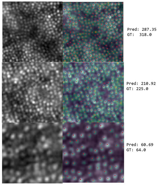
Figure 5.
Sample input and predicted density maps with predicted (Pred) and ground truth (GT) counts (from top) 150 × 150, 128 × 128, and 80 × 80 sizes using IP method. The red dots are the ground truth; the density maps in green overlaid on the original image are the predicted density maps.
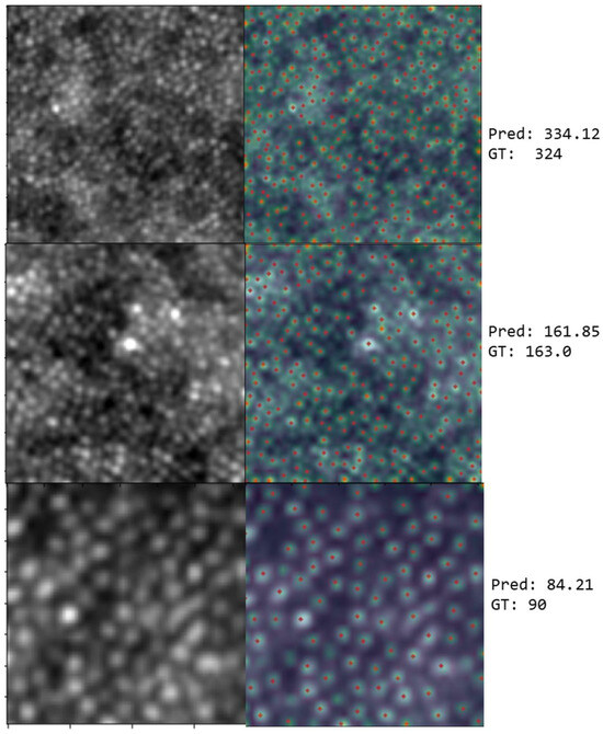
Figure 6.
Sample input and predicted density maps with predicted (Pred) and ground truth (GT) counts (from top) 150 × 150, 128 × 128, and 80 × 80 sizes using the L2R method. The red dots are the ground truth, and the density maps in green overlaid on the original image are the predicted density maps.
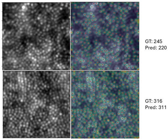
Figure 7.
Sample input and predicted density maps with predicted (Pred) and ground truth (GT) counts (from top) 150 × 150 using the IP + L2R (top) and MTSSL (bottom) method. The red dots are the ground truth, and the density maps in green overlaid on the original image are the predicted density maps.
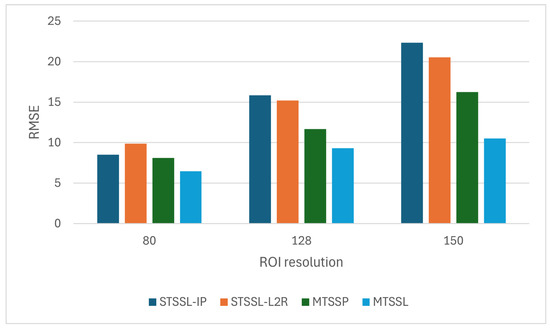
Figure 8.
Results showing RMSE metrics of the IP, L2R, MTSSP, and MTSSL methods on different ROI resolutions.
Wilcoxon signed-rank statistical tests were performed to see if the improvements were significant. We observed that MTSSL achieved significantly lower RMSE than IP (p = 0.012), L2R (p = 0.019), and MTSSP (p = 0.0345). Therefore, we conclude that MTSSL’s improvement is statistically significant at 95% confidence interval. However, IP and L2R (p = 0.058) did not show a significant difference at .
In addition to predictive performance, we assessed MTSSL’s computational complexity under our experimental setup. The model comprises 62 M parameters and performs approximately 41.57 GFLOPs per image forward pass. All the experiments were conducted on a Lambda QUAD deep learning workstation with AMD EPYC 7513 32-Core Processor, 4 NVIDIA A100-SXM4-80 GB GPUs. The training time was observed to be 11.8 s/iteration, and inference was 0.4 s/iteration or 12.5 ms per image latency. Figure 9 illustrates the training run time and the inference times of each method.
Figure 9.
Runtime charts showing training and validation times for each method.
4.2. Counting Performance in Different Regions
The performance of MTSSL was also assessed in different regions of the image shown in Figure 10. Since the cone distribution varies across regions, we observed that in areas blurred due to densely packed cones, the model’s performance declined. Additionally, cloudy regions and low resolution contributed to misdetections. To assess this, a 1500 × 1500 image was divided into 150 × 150 patches. Density maps were generated for each patch and then combined back to reconstruct the full-resolution image. The total counts were grouped into five percentile-based buckets: two below the average and two above, spanning the 20th, 40th, and up to the 100th percentiles. Regions with lower cone predictions are shown near the fovea or along the border regions where blurring was more prominent.
Figure 10.
Spatial distribution of cones through predicted density maps in various regions of a 1500 × 1500 image captured using retinal camera.
4.3. Performance of IP-Related Self-Supervised Tasks vs. Counting Performance
The STSSL-IP task was evaluated across different numbers of pretraining epochs. We observed that increasing the number of epochs led to lower reconstruction error, indicating improved performance on the pretext task. However, this did not always translate to better downstream counting accuracy, suggesting a trade-off. Excessive pretraining on inpainting may bias the model toward low-level reconstruction features, potentially hindering its ability to generalize for the counting task, as shown in Figure 11.
Figure 11.
Change in downstream performance with increase in pretraining epochs of IP, along with reconstruction error and PSNR measures.
In a similar setting, when the IP task was used in conjunction with L2R and integrated into the full MTSSL framework, we observed that the varying complexities of the individual tasks caused them to converge at different rates. This discrepancy hindered the model’s ability to effectively learn shared representations, as one task could dominate the optimization process before others had sufficiently contributed. To address this, we adopted a sequential learning [48] strategy where the MTSSL model was trained initially only with IP loss for 50 epochs to allow stable learning of contextual representations before incorporating the remaining losses. The significance of improving the IP task early, especially in capturing pixel-level structural details, was reflected in the quality of the generated density maps. As shown in Figure 12, increasing the number of pretraining epochs for the IP task within the combined setup led to sharper and more accurate density maps, with the image on the bottom trained on a sequential setting.
Figure 12.
Improvement in density maps with sequential learning (bottom) of IP in MTSSL.
4.4. Point Map Localization
The point localization was performed on the predicted density maps. The quantitative results were evaluated using precision, recall, F1-score, and localization error of the two employed methods compared to the ground truth. While the L2R method performed better than IP in count estimation, the localization performance of the L2R-generated density maps was poor compared to IP. We observe that PLM and SS approaches showed similar scores, with SS showing slightly better scores. However, the MTSSL method produced density maps where PLM also showed better localization. The scores for different approaches are illustrated in Figure 13. The mean localization error was observed to be 2.1 for MTSSL, 2.7 for MTSSP, and 3.4 and 3.5 for IP and L2R methods. The results show that MTSSL improves the localization performance from density maps, where density maps produced by L2R show the worst F1-score localization performance.
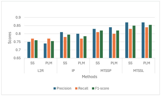
Figure 13.
Point Localization Metrics.
4.5. Ablations
To assess the individual contributions of each component in MTSSL, we performed component analysis by removing components and generating different models with the component combinations as shown in Table 1. The results show that each component contributes to improving the performance, and the overall performance of MTSSL is due to the fusion of these components. The improvement from M1 to M3 indicates that employing generative context-aware learning has enabled learning pixel-wise features along with global understanding and distribution features in the image. The improvement of M4 over M1 suggests that learning global hierarchical ranking of patches introduces inductive bias to the model to distinguish the patches by their counts, contributing to counting accuracy. The integration of generative and predictive pretraining tasks proved effective in capturing local features and global context required for object counting.

Table 1.
Comparison of models with various loss functions and RMSE values.
To effectively balance the individual losses within the joint optimization of MTSSL, we performed a sensitivity analysis on the lambda hyperparameters to examine how hyperparameter variations influence model performance. Specifically, we varied one hyperparameter at a time while fixing the others at their optimal values and observed the resulting changes in the model’s performance. The optimal values were determined using grid search. Figure 14 illustrates how the RMSE scores respond to these hyperparameter adjustments, highlighting the model’s sensitivity and associated uncertainty concerning each parameter. We observe that changing the hyperparameters from their optimal values affects the RMSE scores. The sensitivity arises from how each component learns features that contribute to the overall model performance. Increasing and might encourage the model to focus more on task-specific details, but this could also reduce its overall performance. Decreasing the values weakens the model’s ability to learn enough features that contribute to counting. Increasing and reducing cause density maps to merge close or noisy areas, thereby reducing the model performance. Overall, the three parameters in MTSSL can be tuned within a practical range to regulate the impact of each loss component on model performance. Systematically identifying their optimal values ensures a balanced trade-off among the inpainting, ranking, and density-estimation objectives, yielding peak performance. This sensitivity analysis guides the tailoring of MTSSL to different applications.
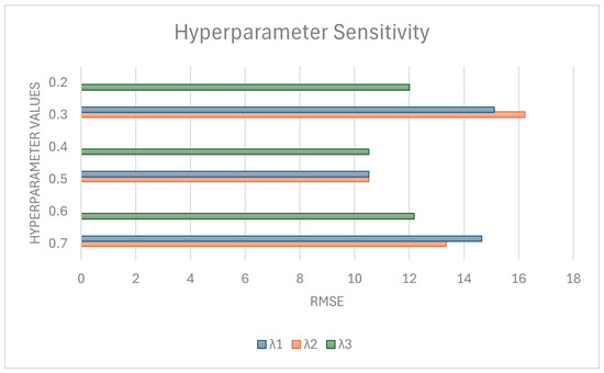
Figure 14.
Sensitivity analysis for different parameter values.
To evaluate the generalizability of the model, a subset of images without noise was chosen, and Gaussian noise was applied to observe the model’s performance in a controlled setting. This was helpful to assess the applicability of the model on different regions of the image based on the noise levels. Figure 15 shows that the count error increases with an increase in noise.
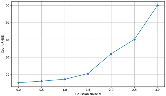
Figure 15.
Noise vs. RMSE.
The L2R and IP networks were also finetuned with the AOSLO dataset to evaluate the generality of the methods. However, these images were only used to finetune the IP and L2R models pretrained on the AO dataset, and not the MT-SSL method, as this also requires unlabeled data. When finetuned on AOSLO of patch sizes 150 × 150, the IP method gave an RMSE of 8.84 and L2R 12.04. Figure 16 shows samples of AOSLO and predictions.
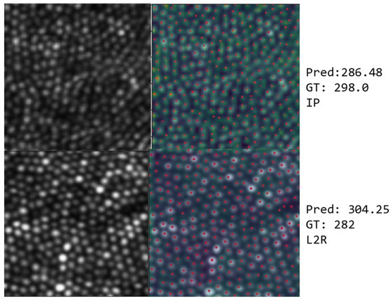
Figure 16.
Sample input and predicted density maps along with predicted (Pred) and ground truth (GT) counts of AOSLO images (from top) IP and L2R methods. The red dots are the ground truth, and the density maps in green overlaid on the original image are the predicted density maps.
5. Discussion
The results demonstrate that the proposed MTSSL approach significantly reduced the counting error RMSE by a factor of 2 compared to the individual SSL tasks and by a factor of compared to the MTSSP approach, as shown in Figure 8. Even with the reduced dataset size, the MTSSL approach achieved an RMSE of , outperforming all other methods. For patch sizes 128 × 128, the RMSE was observed to be , , and when finetuned on the models pretrained on 150 × 150 patches for IP, L2R, and MTSSP, respectively. A combination of different patch sizes for unlabeled and labeled data in the MTSSL setup resulted in degraded performance.
DT is a deterministic approach and requires careful parameter selection for each patch to avoid misdetections of cones. Determining the region of interest points also depends on the Gaussian filter threshold and resized patch size. This is especially challenging when the images are blurry and noisy. We observed a significant decrease in the performance of the DT as patch size increased. At a patch size of 150, the RMSE of DT was observed to be 48.03, compared to MTSSL, which reduced this error roughly by a factor of five.
The IP method was tested with single patch masking; sample reconstructions are shown in Figure 17. The context learning aided in understanding the image background and morphological characteristics of cones within that patch and in reconstructing the masked patch accordingly. However, the model could not reconstruct the exact spatial distribution within the masked region in the current experimental setting.
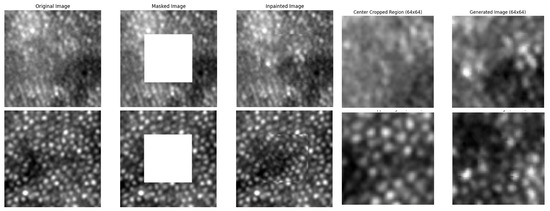
Figure 17.
Sample inpainting outputs, with original, masked, inpainted, masked part, and reconstructed masked part from left to right.
When comparing L2R and IP methods, it was observed that L2R produced lower RMSE compared to the IP method. However, the density maps generated by the IP method exhibited sharper and more distinct delineation of the cone regions compared to the L2R method. Additionally, the L2R method exhibited slightly poor performance when finetuned with the AOSLO dataset compared to the IP method.
Furthermore, despite achieving low RMSE, the L2R demonstrated slightly lower compared to the IP method, indicating that the IP method was more effective in capturing the variability of the counts. Upon inference with 128 × 128 and 80 × 80 patch sizes using the finetuned models, IP yielded better results than L2R. These observations suggest that the L2R method has lower generalizability compared to the IP method.
From the results, we posit that L2R, with its design specifically tailored for counting purposes during the pretraining, possesses superior capability in regressing counts accurately; however, it was not able to capture the features of cones as efficiently as the IP method. On the other hand, IP exhibited superior performance in capturing the variability of the data and generating quality density maps. Variability in cone distribution density is used for disease detection and management. These maps further aided in producing better point maps as compared to those in the L2R method. Sample density maps are shown in Figure 18. This disparity may stem from the reasons that inpainting enables the learning of the structures and distribution of cones in the images.
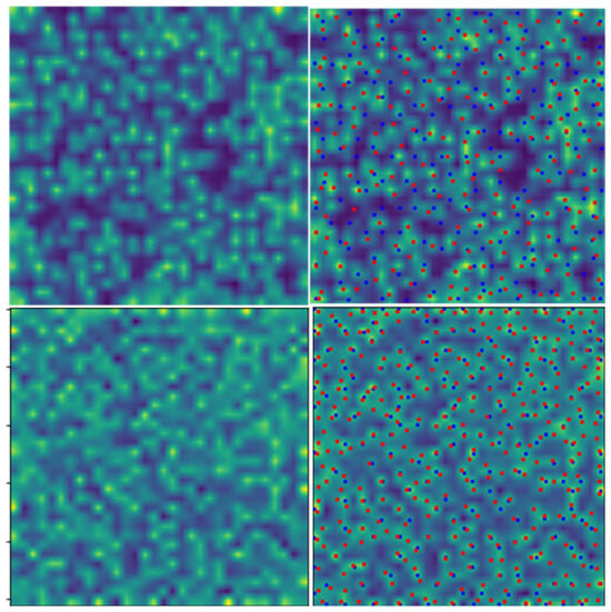
Figure 18.
Predicted density maps to the left and localization of cones shown to the right, where red dots represent the Gaussian threshold method, and the blue dots represent localizations using the OTM method.
The combination of these two methods yielded better results for both regression and generating quality density maps for point localization where the RMSE improved by a factor of 2 and localization F1 score improved from 0.76 to 0.85. The proposed MTSSL approach outperformed the other three methods, as shown in Table 2, demonstrating a better reduction in counting error. Notably, even with a 30% reduction in dataset size, it continued to outperform the alternatives. The two-stage approach, where a pretrained encoder is frozen and only the decoder is finetuned, was able to introduce count-related inductive biases and aid in improving the downstream task to some extent. However, because the counting task was optimized separately, it could retain pretext-task-specific representations without fully adapting to the downstream counting objective. In contrast, the proposed joint optimization in MTSSL guided the network to learn general-purpose count-relevant features from unlabeled data, particularly with pixel-wise reconstruction and global ranking to compare counts among the patches, while simultaneously supervising the density estimation task. This highlights the effectiveness of combining hybrid pretext tasks in a unified multi-task semi-supervised learning framework. Additionally, though combined loss helped in improving the counting performance, it struggled with providing optimal results for the complex task within the experimental setup. A tradeoff of improving task-specific features with the target task is necessary, and techniques like employed sequential learning can prove advantageous in such scenarios.
Table 2.
Performance metrics for different models. The results are presented in the format of ().
In the context of localization, the Sinkhorn-based method yielded better point maps compared to estimating peak local maxima. Peak local maxima also performed better as the quality of density maps improved with MTSSL. It is particularly challenging in the AO images, where the background contains noise, blur, or cloudy regions, which can hinder the sharp delineation of cones in the density map. In such scenarios, mere peak estimation might not be efficient. However, all the methods have a scope for improvement to accurately position the locations at the center of cones. This could be a potential area to explore to directly produce the point maps instead of designing a post-processing step.
6. Conclusions
In this work, we proposed a novel unified hybrid multi-task semi-supervised learning framework for cone counting and density estimation in AO rtx1 images. By jointly optimizing two self-supervised pretext tasks—image inpainting and learning-to-rank, alongside a supervised density estimation task—our approach effectively leverages both unlabeled and limited labeled data. The proposed framework introduces strong inductive biases relevant to the counting task and encourages the learning of generalizable, task-aligned representations. Experimental results demonstrate that MTSSL consistently outperforms individual self-supervised two-stage finetuning approaches, achieving significantly lower counting errors, even when the dataset size is reduced. The proposed approach can be further extended to study disparities in cone structures or distribution associated with retinal diseases, enabling quantitative analysis of pathological changes. Overall, these results highlight the potential of MTSSL to advance label-efficient learning for dense object counting tasks in medical imaging and other domains. While MTSSL showed improved performance, the generalizability of the approach for different scales is limited and requires the model to be trained for each different scale. Also, the post-processing step to localize the center of cones leads to cascading errors. Adopting end-to-end pipelines and improving the generalizability for different scales would guide future extensions of our framework.
Author Contributions
Conceptualization, V.B., A.A., P.C. and M.S.; Methodology, V.B. and M.S.; Software, V.B.; Validation, A.A.; Investigation, V.B. and A.A.; Resources, P.C., Q.D.N. and M.S.; Data curation, A.A. and Q.D.N.; Writing—original draft, V.B.; Writing—review & editing, V.B. and M.S.; Visualization, V.B.; Supervision, P.C. and M.S. All authors have read and agreed to the published version of the manuscript.
Funding
This research received no external funding.
Informed Consent Statement
Not applicable.
Data Availability Statement
Any inquiry regarding the private dataset should be made to the corresponding authors.
Acknowledgments
The authors would like to acknowledge Dilanga Abeyrathna for supporting with the formatting and figures in the manuscript.
Conflicts of Interest
The authors declare no conflicts of interest.
References
- Majumder, P.D.; Marchese, A.; Pichi, F.; Garg, I.; Agarwal, A. An update on autoimmune retinopathy. Indian J. Ophthalmol. 2020, 68, 1829. [Google Scholar] [CrossRef]
- Campochiaro, P.A.; Mir, T.A. The mechanism of cone cell death in Retinitis Pigmentosa. Prog. Retin. Eye Res. 2018, 62, 24–37. [Google Scholar] [CrossRef] [PubMed]
- Chen, Y.; Ratnam, K.; Sundquist, S.M.; Lujan, B.; Ayyagari, R.; Gudiseva, V.H.; Roorda, A.; Duncan, J.L. Cone photoreceptor abnormalities correlate with vision loss in patients with Stargardt disease. Investig. Ophthalmol. Vis. Sci. 2011, 52, 3281–3292. [Google Scholar] [CrossRef]
- Davidson, B.; Kalitzeos, A.; Carroll, J.; Dubra, A.; Ourselin, S.; Michaelides, M.; Bergeles, C. Automatic cone photoreceptor localisation in healthy and Stargardt afflicted retinas using deep learning. Sci. Rep. 2018, 8, 7911. [Google Scholar] [CrossRef]
- Tang, J.; Liu, H.; Mo, S.; Zhu, Z.; Huang, H.; Liu, X. Cone Density Distribution and Related Factors in Patients Receiving Hydroxychloroquine Treatment. Investig. Ophthalmol. Vis. Sci. 2023, 64, 29. [Google Scholar] [CrossRef]
- Toledo-Cortés, S.; Dubis, A.M.; González, F.A.; Müller, H. Deep Density Estimation for Cone Counting and Diagnosis of Genetic Eye Diseases From Adaptive Optics Scanning Light Ophthalmoscope Images. Transl. Vis. Sci. Technol. 2023, 12, 25. [Google Scholar] [CrossRef]
- Vera-Díaz, F.A.; Doble, N. The Human Eye and Adaptive Optics. In Topics in Adaptive Optics; Tyson, R.K., Ed.; IntechOpen: Rijeka, Croatia, 2012; Chapter 6. [Google Scholar] [CrossRef]
- Burns, S.A.; Elsner, A.E.; Sapoznik, K.A.; Warner, R.L.; Gast, T.J. Adaptive optics imaging of the human retina. Prog. Retin. Eye Res. 2019, 68, 1–30. [Google Scholar] [CrossRef]
- Samelska, K.; Szaflik, J.P.; Śmigielska, B.; Zaleska-Żmijewska, A. Progression of Rare Inherited Retinal Dystrophies May Be Monitored by Adaptive Optics Imaging. Life 2023, 13, 1871. [Google Scholar] [CrossRef] [PubMed]
- Nakanishi, A.; Ueno, S.; Kawano, K.; Ito, Y.; Kominami, T.; Yasuda, S.; Kondo, M.; Tsunoda, K.; Iwata, T.; Terasaki, H. Pathologic changes of cone photoreceptors in eyes with occult macular dystrophy. Investig. Ophthalmol. Vis. Sci. 2015, 56, 7243–7249. [Google Scholar] [CrossRef]
- Kupis, M.; Wawrzyniak, Z.M.; Szaflik, J.P.; Zaleska-Żmijewska, A. Retinal Photoreceptors and Microvascular Changes in the Assessment of Diabetic Retinopathy Progression: A Two-Year Follow-Up Study. Diagnostics 2023, 13, 2513. [Google Scholar] [CrossRef] [PubMed]
- Mc Grath, O.; Sarfraz, M.W.; Gupta, A.; Yang, Y.; Aslam, T. Clinical utility of artificial intelligence algorithms to enhance wide-field optical coherence tomography angiography images. J. Imaging 2021, 7, 32. [Google Scholar] [CrossRef]
- Legras, R.; Gaudric, A.; Woog, K. Distribution of cone density, spacing and arrangement in adult healthy retinas with adaptive optics flood illumination. PLoS ONE 2018, 13, e0191141. [Google Scholar] [CrossRef]
- Cunefare, D.; Huckenpahler, A.L.; Patterson, E.J.; Dubra, A.; Carroll, J.; Farsiu, S. RAC-CNN: Multimodal deep learning based automatic detection and classification of rod and cone photoreceptors in adaptive optics scanning light ophthalmoscope images. Biomed. Opt. Express 2019, 10, 3815–3832. [Google Scholar] [CrossRef]
- Cunefare, D.; Langlo, C.S.; Patterson, E.J.; Blau, S.; Dubra, A.; Carroll, J.; Farsiu, S. Deep learning based detection of cone photoreceptors with multimodal adaptive optics scanning light ophthalmoscope images of achromatopsia. Biomed. Opt. Express 2018, 9, 3740–3756. [Google Scholar] [CrossRef] [PubMed]
- Morgan, J.I.; Chen, M.; Huang, A.M.; Jiang, Y.Y.; Cooper, R.F. Cone identification in choroideremia: Repeatability, reliability, and automation through use of a convolutional neural network. Transl. Vis. Sci. Technol. 2020, 9, 40. [Google Scholar] [CrossRef] [PubMed]
- Smith, T.B.; Smith, N. Detection of cone photoreceptors in adaptive optics retinal images using topographical features and machine learning. In Proceedings of the Classical Optics 2014, Kohala Coast, HI, USA, 22–26 June 2014; Optica Publishing Group: Washington, DC, USA, 2014; p. JTu5A.41. [Google Scholar] [CrossRef]
- Hamwood, J.; Alonso-Caneiro, D.; Sampson, D.M.; Collins, M.J.; Chen, F.K. Automatic detection of cone photoreceptors with fully convolutional networks. Transl. Vis. Sci. Technol. 2019, 8, 10. [Google Scholar] [CrossRef]
- Garrioch, R.; Langlo, C.; Dubis, A.M.; Cooper, R.F.; Dubra, A.; Carroll, J. Repeatability of in vivo parafoveal cone density and spacing measurements. Optom. Vis. Sci. 2012, 89, 632–643. [Google Scholar] [CrossRef]
- Zaleska-Żmijewska, A.; Wawrzyniak, Z.M.; Dąbrowska, A.; Szaflik, J.P. Adaptive optics (rtx1) high-resolution imaging of photoreceptors and retinal arteries in patients with diabetic retinopathy. J. Diabetes Res. 2019, 2019, 9548324. [Google Scholar] [CrossRef]
- Morgan, J.I.; Vergilio, G.K.; Hsu, J.; Dubra, A.; Cooper, R.F. The reliability of cone density measurements in the presence of rods. Transl. Vis. Sci. Technol. 2018, 7, 21. [Google Scholar] [CrossRef] [PubMed]
- Akhavanrezayat, A.; Bommanapally, V.; Mudiyanselage, D.L.G.; Halim, M.S.; Or, C.; Karaca, I.; Uludag, G.; Yavari, N.; Bazojoo, V.; Mobasserian, A.; et al. A novel objective method to detect the foveal center point in the rtx1TM device using artificial intelligence. Investig. Ophthalmol. Vis. Sci. 2023, 64, 1068. [Google Scholar]
- Bommanapally, V.; Abeyrathna, D.; Chundi, P.; Subramaniam, M. Super resolution-based methodology for self-supervised segmentation of microscopy images. Front. Microbiol. 2024, 15, 1255850. [Google Scholar] [CrossRef]
- Abeyrathna, D.; Ashaduzzaman, M.; Malshe, M.; Kalimuthu, J.; Gadhamshetty, V.; Chundi, P.; Subramaniam, M. An AI-based approach for detecting cells and microbial byproducts in low volume scanning electron microscope images of biofilms. Front. Microbiol. 2022, 13, 996400. [Google Scholar] [CrossRef] [PubMed]
- Deng, L.; Zhou, Q.; Wang, S.; Górriz, J.M.; Zhang, Y. Deep learning in crowd counting: A survey. CAAI Trans. Intell. Technol. 2024, 9, 1043–1077. [Google Scholar] [CrossRef]
- Liu, X.; Van De Weijer, J.; Bagdanov, A.D. Leveraging unlabeled data for crowd counting by learning to rank. In Proceedings of the IEEE Conference on Computer Vision and Pattern Recognition, Salt Lake City, UT, USA, 18–23 June 2018; pp. 7661–7669. [Google Scholar]
- Babu Sam, D.; Agarwalla, A.; Joseph, J.; Sindagi, V.A.; Babu, R.V.; Patel, V.M. Completely self-supervised crowd counting via distribution matching. In Proceedings of the European Conference on Computer Vision, Tel Aviv, Israel, 23–27 October 2022; Springer: Cham, Switzerland, 2022; pp. 186–204. [Google Scholar]
- Bommanapally, V.; Akhavanrezayat, A.; Nguyen, Q.D.; Subramaniam, M. COINS: Counting Cones Using Inpainting Based Self-supervised Learning. In Proceedings of the 2024 46th Annual International Conference of the IEEE Engineering in Medicine and Biology Society (EMBC), Orlando, FL, USA, 15–19 July 2024; pp. 1–4. [Google Scholar]
- Sun, G.; Liu, Y.; Probst, T.; Paudel, D.P.; Popovic, N.; Gool, L. Rethinking global context in crowd counting. Mach. Intell. Res. 2024, 21, 640–651. [Google Scholar] [CrossRef]
- Ma, Z.; Zhou, L.; Wu, D.; Zhang, X. A small object detection method with context information for high altitude images. Pattern Recognit. Lett. 2025, 188, 22–28. [Google Scholar] [CrossRef]
- Zhao, T.; Yue, Y.; Sun, H.; Li, J.; Wen, Y.; Yao, Y.; Qian, W.; Guan, Y.; Qi, S. MAEMC-NET: A hybrid self-supervised learning method for predicting the malignancy of solitary pulmonary nodules from CT images. Front. Med. 2025, 12, 1507258. [Google Scholar] [CrossRef]
- Pathak, D.; Krahenbuhl, P.; Donahue, J.; Darrell, T.; Efros, A.A. Context encoders: Feature learning by inpainting. In Proceedings of the IEEE Conference on Computer Vision and Pattern Recognition, Las Vegas, NV, USA, 26 June–1 July 2016; pp. 2536–2544. [Google Scholar]
- Ching, J.H.; See, J.; Wong, L.K. Learning image aesthetics by learning inpainting. In Proceedings of the 2020 IEEE International Conference on Image Processing (ICIP), Abu Dhabi, United Arab Emirates, 25–28 October 2020; pp. 2246–2250. [Google Scholar]
- Heinrich, K.; Roth, A.; Zschech, P. Everything counts: A Taxonomy of Deep Learning Approaches for Object Counting. In Proceedings of the ECIS, Stockholm, Sweden, 8–14 June 2019. [Google Scholar]
- Liao, W.; Xiong, H.; Wang, Q.; Mo, Y.; Li, X.; Liu, Y.; Chen, Z.; Huang, S.; Dou, D. Muscle: Multi-task self-supervised continual learning to pre-train deep models for x-ray images of multiple body parts. In Proceedings of the International Conference on Medical Image Computing and Computer-Assisted Intervention, Singapore, 18–22 September 2022; Springer: Berlin/Heidelberg, Germany, 2022; pp. 151–161. [Google Scholar]
- Crawshaw, M. Multi-task learning with deep neural networks: A survey. arXiv 2020, arXiv:2009.09796. [Google Scholar] [CrossRef]
- Xie, Q.; Dai, Z.; Hovy, E.; Luong, T.; Le, Q. Unsupervised data augmentation for consistency training. Adv. Neural Inf. Process. Syst. 2020, 33, 6256–6268. [Google Scholar]
- Gu, S.; Lian, Z. A unified multi-task learning framework of real-time drone supervision for crowd counting. arXiv 2022, arXiv:2202.03843. [Google Scholar]
- Zhu, P.; Li, J.; Cao, B.; Hu, Q. Multi-task credible pseudo-label learning for semi-supervised crowd counting. IEEE Trans. Neural Netw. Learn. Syst. 2023, 35, 10394–10406. [Google Scholar] [CrossRef] [PubMed]
- Berthelot, D.; Carlini, N.; Goodfellow, I.; Papernot, N.; Oliver, A.; Raffel, C.A. Mixmatch: A holistic approach to semi-supervised learning. Adv. Neural Inf. Process. Syst. 2019, 32, 5050–5060. [Google Scholar]
- Wang, Y.; Song, D.; Wang, W.; Rao, S.; Wang, X.; Wang, M. Self-supervised learning and semi-supervised learning for multi-sequence medical image classification. Neurocomputing 2022, 513, 383–394. [Google Scholar] [CrossRef]
- Qiu, Z.; Zeng, W.; Liao, D.; Gui, N. A-SFS: Semi-supervised feature selection based on multi-task self-supervision. Knowl.-Based Syst. 2022, 252, 109449. [Google Scholar] [CrossRef]
- Pfister, J.; Kobs, K.; Hotho, A. Self-supervised multi-task pretraining improves image aesthetic assessment. In Proceedings of the IEEE/CVF Conference on Computer Vision and Pattern Recognition, Nashville, TN, USA, 20–25 June 2021; pp. 816–825. [Google Scholar]
- Fang, X.; Zhang, G.; Zhang, G.; Zhou, X.; Wu, J.; Zhao, L. A hybrid self-supervised learning framework for hyperspectral image classification. In Proceedings of the 2023 International Conference on Computer, Vision and Intelligent Technology, Chenzhou, China, 25–28 August 2023; pp. 1–7. [Google Scholar]
- Lin, W.; Chan, A.B. Optimal transport minimization: Crowd localization on density maps for semi-supervised counting. In Proceedings of the IEEE/CVF Conference on Computer Vision and Pattern Recognition, Vancouver, BC, Canada, 17–24 June 2023; pp. 21663–21673. [Google Scholar]
- Bidaut Garnier, M.; Flores, M.; Debellemanière, G.; Puyraveau, M.; Tumahai, P.; Meillat, M.; Schwartz, C.; Montard, M.; Delbosc, B.; Saleh, M. Reliability of cone counts using an adaptive optics retinal camera. Clin. Exp. Ophthalmol. 2014, 42, 833–840. [Google Scholar] [CrossRef]
- Li, Y.; Zhang, X.; Chen, D. Csrnet: Dilated convolutional neural networks for understanding the highly congested scenes. In Proceedings of the IEEE Conference on Computer Vision and Pattern Recognition, Salt Lake City, UT, USA, 18–22 June 2018; pp. 1091–1100. [Google Scholar]
- Shi, C.; Sun, C.; Wu, Y.; Jia, Y. Video anomaly detection via sequentially learning multiple pretext tasks. In Proceedings of the IEEE/CVF International Conference on Computer Vision, Paris, France, 1–6 October 2023; pp. 10330–10340. [Google Scholar]


Disclaimer/Publisher’s Note: The statements, opinions and data contained in all publications are solely those of the individual author(s) and contributor(s) and not of MDPI and/or the editor(s). MDPI and/or the editor(s) disclaim responsibility for any injury to people or property resulting from any ideas, methods, instructions or products referred to in the content. |
© 2025 by the authors. Licensee MDPI, Basel, Switzerland. This article is an open access article distributed under the terms and conditions of the Creative Commons Attribution (CC BY) license (https://creativecommons.org/licenses/by/4.0/).