Abstract
The evaluation of pressure drops across the length of production wells is a crucial task, as it influences both the cost-effective selection of tubing and the development of an efficient production strategy, both of which are vital for maximizing oil recovery while minimizing operational expenses. To address this, our study proposes an innovative hybrid intelligent system designed to predict bottom-hole flowing pressure in vertical multiphase conditions with superior accuracy compared to existing methods using a data set of 150 field measurements amassed from Algerian fields. In this work, the applied hybrid framework is the Adaptive Neuro-Fuzzy Inference System (ANFIS), which integrates artificial neural networks (ANN) with fuzzy logic (FL). The ANFIS model was constructed using a subtractive clustering technique after data filtering, and then its outcomes were evaluated against the most widely utilized correlations and mechanistic models. Graphical inspection and error statistics confirmed that ANFIS consistently outperformed all other approaches in terms of precision, reliability, and effectiveness. For further improvement of the ANFIS performance, a particle swarm optimization (PSO) algorithm is employed to refine the model and optimize the design of the antecedent Gaussian memberships along with the consequent linear coefficient vector. The results achieved by the hybrid ANFIS-PSO model demonstrated greater accuracy in bottom-hole pressure estimation than the conventional hybrid approach.
1. Introduction
The instantaneous flow of liquids and gases, or multi-phase flow, is common in the petroleum engineering installations such as tubing, pipelines, separators, treaters, and heat exchangers, and problems associated with such flow have been of interest for a long time [1]. In oil wells, the prevailing phase conditions often shift along the flow path toward the surface. At bottom-hole conditions, the stream may remain single-phase due to the high pressure; however, as pressure decreases with elevation in the wellbore, dissolved gas is progressively released from the liquid, leading to multiphase behavior. Even in gas wells, liquid condensates or formation water may be produced alongside the gas. These factors explain why multiphase flow is so commonly encountered in well systems [2]. Accurate pressure drop prediction is vital in designing well completions, artificially lift systems, and also well production monitoring [3]. Since multiphase flow is highly complex, pressure-drop estimation has typically been approached through empirical or semi-empirical correlations [4]. However, in multiphase systems, pressure-drop estimation challenging due to the strong interdependence among the governing variables. Some of these variables are flow pattern, holdup, pipe size and orientation, fluid properties, and flow rates of the different phases [5]. Numerous approaches have been suggested for estimating pressure drop in vertical multiphase flow. These range from purely empirical correlations to semi-empirical, mechanistic formulations. While the empirical models are derived from experimental observations and data fitting, the mechanistic ones rely on fundamental physical principles to describe the flow and therefore offered a certain degree of reliability [6]. There is currently no universal correlation or mechanistic model that remains valid for every production scenario including gas oil ratio (GOR), tubing size, water cut, and liquid rate [3]; they only work well under certain conditions. In the majority of Algerian fields, two-phase flow is widely encountered during the production process; in addition, most of the Algerian field wells in these reservoirs were completed with large-diameter tubing to handle the high production rates. However, such operating conditions differ from those assumed in the development of most existing correlations. In an effort to tackle the complicated issues, we must go beyond the standard numerical procedures. As an alternative, conventional analytical methods can be complemented by emerging approaches and artificial intelligence techniques, including neural networks [7], fuzzy logic, and evolutionary algorithms, which provide high efficiency to resolve real world problems [8,9,10].
Recent research has increasingly used machine learning techniques to refine bottom-hole pressure prediction in oil and gas production. These studies address the limitations of conventional mechanistic correlations, particularly under complex multiphase flow and variable wellbore conditions. For example, ref. [11] proposed a hybrid deep learning framework that integrates LSTM and CNN networks for BHP forecasting in managed pressure drilling (MPD), achieving significantly improved accuracy compared to traditional models. Similarly, ref. [12] utilized multivariate adaptive regression splines (MARS) for BHP prediction, offering interpretable models with strong performance (R ≈ 0.94).
Beyond purely neural models, other techniques such as eXtreme Gradient Boosting (XGBoost) have been explored. A recent study by [13] demonstrated XGBoost can outperform conventional ML algorithms in carbonate formations, where flow behavior is highly nonlinear and heterogeneous. In another direction, ref. [14] introduced a transparent ANN-based formulation to enable real-time forecasting while retaining interpretability.
Furthermore, several hybrid approaches have emerged to combine data-driven learning with smart production data. For instance, the work of [15] highlighted the integration of real-time production analytics with ML to improve prediction in unconventional reservoirs. These efforts underscore the trend toward hybrid intelligent systems capable of handling uncertainty, nonlinear flow dynamics, and limited data sets.
In continuation of prior studies utilizing machine learning-based BHP prediction, this study introduces—for the first time—a hybrid PSO–ANFIS model specifically developed to enhance the accuracy, robustness, and interpretability of bottom-hole pressure estimation, while requiring minimal parameter tuning.
This study outlines a two-part strategy. The first part employs an Adaptive Neuro-Fuzzy Inference System (ANFIS) is implemented to construct a reliable predictive model for estimating bottom-hole flowing pressure during the natural flow of multiphase fluids through tubing in vertical wells. Among several soft computing techniques explored, ANFIS was selected due to its ability to incorporate expert knowledge via fuzzy logic and adapt its structure through learning. The output of the ANFIS model is compared to eight commonly used mechanistic flow correlations in order to evaluate its predictive power: Mukherjee and Brill, Duns and Ros, Aziz et al., Hagedorn and Brown, Ansari et al., Beggs and Brill, Orkiszewski, and Gray [16,17,18,19,20,21,22,23]. The evaluation is based on several statistical performance metrics to ensure a comprehensive assessment of model validity.
In the second part, the ANFIS model was trained with the PSO algorithm on the same data set, replacing the standard hybrid learning strategy that combines back propagation (BP) and least squares estimation (LSE). We employ PSO to simultaneously optimize both the consequent linear parameters and the antecedent membership function parameters of the ANFIS network. This optimization process aims to improve convergence stability and model generalization. Finally, a comparative analysis is conducted between the PSO-optimized ANFIS and the standard ANFIS trained using the LS–BP hybrid method, showcasing the suggested method’s performance benefits.
2. Methods
2.1. Adaptive Neuro-Fuzzy Inference System
Jang was the first to introduce the ANFIS [24], as a hybrid modeling technique that integrates the reasoning mechanisms of fuzzy logic with the learning capabilities of neural networks. The Takagi–Sugeno (T–S) fuzzy inference system serves as the foundation for the ANFIS and is designed to leverage the strengths of both approaches in a unified framework. Specifically, it combines fuzzy logic thinking and neural network counting.
The ANFIS model employs a set of “If–Then” fuzzy rules and adapts its internal parameters through a learning process to approximate complex nonlinear functions. The primary goal is to estimate an output ŷ that closely matches the actual output y for a given input vector. Due to this adaptive nature and approximation capability, the ANFIS is considered a universal function estimator [24].
The ANFIS architecture is composed of five layers that incorporate two categories of nodes: square nodes and circular nodes. Square nodes contain adaptable parameters and represent either the linear functions in the fuzzy rules’ consequent section or the membership functions (MFs) in the antecedent part. Circular nodes, on the other hand, have fixed parameters and serve as intermediate processing units that link antecedents to consequents. An important feature of ANFIS is its interpretability. Unlike typical black-box neural networks, ANFIS retains the transparency of a fuzzy inference system, allowing the model to be expressed in terms of human-understandable linguistic rules [25]. Figure 1 illustrates the typical ANFIS architecture as a multi-layered network composed of five distinct computational layers.
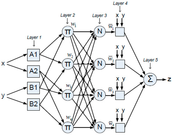
Figure 1.
Two inputs each with 2 MFs in the ANFIS model.
- Layer 1: Fuzzification
Convert each input variable into fuzzy sets (Output O) using a MF (μ).
O1,i = μAi (x), i = 1, 2
O1,i−2 = μBi−2 (y), i = 3, 4
In this study the MFs are assumed to be Gaussian.
- Layer 2: Rule Evaluation
Determines the rule’s firing power (wi) by multiplication.
O2,1 = w1 = μA1 (x) ∗ μB1 (x)
O2,2 = w2 = μA1 (x) ∗ μB2 (x)
O2,3 = w3 = μA2(x) ∗ μB1 (x)
O2,4 = w4 = μA2 (x) ∗ μB2 (x)
- Layer 3: Normalization
Computes the ratio of the firing power of the i-th rule (i).
- Layer 4: Consequent Computation
Defines the impact of the i-th rule on the aggregated output.
where pi, qi, and ri are coefficients of consequents of the linear functions fi for the (TKS) fuzzy inference system, respectively.
O4,i = wifi = wi (pi x + qi y + ri) i = 1, 2, 3, 4
- Layer 5: Aggregation
Determines the overall result by adding together the contributions from each rule.
O5 = Σiwifi = Σiwi(pix + qiy + ri)/Σiwi, i = 1, 2, 3, 4
Figure 1 displays the structural design of an ANFIS with two inputs, one output, and four “If−Then” rules. These four rules are defined in Equations (10)–(13).
If X is A1 and Y is B1, then f1 = p1x + q1y + r1
If X is A1 and Y is B2, then f2 = p2x + q2y + r2
If X is A2 and Y is B1, then f3 = p3x + q3y + r3
If X is A2 and Y is B2, then f4 = p4x + q4y + r4
The first part (IF) in the equations is related to the antecedents and the second part (THEN) of the equations to the consequents. While the ANFIS was being trained, these regulations were completed so as to calculate the output of the system.
- Learning Algorithms
Jang [24] proposed four distinct methods for updating the parameters in an ANFIS, each varying in terms of computational complexity and convergence behavior:
- -
- Gradient Descent Only: All parameters—both antecedent and consequent—are updated simultaneously using gradient descent.
- -
- One-Time LSE + Gradient Descent: Initial values are assigned to the parameters, and then the least squares estimator (LSE) is used once for optimizing the consequent parameters, after which all parameters are updated via gradient descent.
- -
- Hybrid Learning (LSE + Gradient Descent): This widely used approach combines forward-pass LSE for consequent parameters with backward-pass gradient descent for antecedent membership function parameters. It offers fast convergence and balanced complexity.
- -
- Extended Kalman Filter (EKF): All parameters are updated using a recursive EKF approach, which generally yields high accuracy at the cost of increased computational load.
In this study, we adopt the hybrid learning algorithm due to its computational efficiency and rapid convergence, making it suitable for modeling bottom-hole pressure in real-time or data-limited applications.
- Performance evaluation
To evaluate the ANFIS model, we used four evaluation metrics known as the average absolute percentage relative deviation (AAPRD %), average absolute deviation error (AADE), correlation coefficient (R2), and standard deviation (SD). These measures are calculated using the difference between the measured (m) and predicted (p) BHP values.
2.2. Particle Swarm Optimization PSO Algorithm
The population-based optimization technique known as particle swarm optimization (PSO) was motivated by the collective social behavior seen in schools of fish and flocks of birds [26]. Kennedy and Eberhart first created the algorithm in 1995, drawing motivation from the field of artificial life and social psychology [27].
A number of practical benefits have led to the widespread use of PSO as an optimization technique [28], including the following:
- -
- Simplicity of implementation: PSO is conceptually straightforward and easy to code.
- -
- Minimal parameter tuning: It requires fewer parameters to be adjusted compared to other metaheuristic algorithms.
- -
- Fast convergence: PSO typically converges quickly toward optimal or near-optimal solutions [29].
- -
- Low computational overhead: It demands significantly less computational effort than many other population-based techniques [30].
- -
- High precision: It can achieve accurate results across a range of problem types.
- -
- Robustness to dimensionality: The algorithm’s performance is not severely degraded by an increase in the number of variables.
Furthermore, PSO has proven effective for many different types of optimization problems, such as multimodal and multi-objective methods, discrete and integer programming [31], and both static [32] and dynamic [33] optimization environments.
In the PSO algorithm, each solution for the problem is represented as a particle inside the search area. Every particle has a fitness value; the higher the fitness, the closer the particle is to the ideal solution. Starting with a swarm of random particles, the PSO iteratively modifies their locations and velocities according to their neighbors’ and their own experiences. Each particle in the swarm maintains a state characterized by two key vectors in each dimension (d): its position (Pid) and velocity (Vid). The PSO algorithm explores the search space by iteratively updating these values based on both individual and collective experiences.
One of the following strategies usually controls particle movement in PSO [34]:
- ➢
- Individual Best (Pbest): Based just on its own historical best position, each particle modifies its velocity.
- ➢
- Global Best (Gbest): Each particle is influenced by the optimal location found by every swarm particle.
- ➢
- Hybrid Strategy: A combination of both individual and global knowledge, allowing a balance between investigating new areas and taking advantage of established, promising ones.
In PSO, the optimization process proceeds through iterative updates of particle positions and velocities. The basic procedure is as follows:
- Step 1: Randomly initialize each particle Pi ∈ P(t) position Xi(t) within the search space, with t = 0.
- Step 2: Use the current position Xi(t) to calculate the fitness F for each particle.
- Step 3: For each particle update the personal best by comparing the current fitness with its previously recorded best:
if F(Xi(t)) < Pbesti, then:
Pbesti = F(Xi(t))
Xpbesti = Xi(t)
- Step 4: Evaluate each individual best fitness against the global best:
if F(xi(t)) < Gbest, then:
Gbest = F(xi(t))
Xgbest = Xi(t)
- Step 5: Update the velocity vector for each particle:
Vi(t) = Vi(t − 1) + ρ1 (Xpbesti − Xi(t)) + ρ2 (Xgbest − Xi(t))
The first term in velocity update equation is referred to as the inertia part, the cognitive module is the second term, and the social module is the last term [28]. R1 and R2 are provided to enhance the searching space with a uniform distribution on [0, 1], where ρ1 and ρ2 are random variables defined as ρ1 = R1C1 and ρ2 = R2C2. C1 and C2 are positive acceleration constants that fall in the range 1–3, where C1 represents the confidence a particle has in itself, thus promoting exploration, while C2 represents the confidence a particle has in its neighbors, thereby promoting exploitation.
- Step 6: Update each particle position:
Xi(t) = Xi(t − 1) + Vi(t)
t = t + 1
- Step 7: Repeat from Step 2 until convergence is achieved.
Given that the velocity update equations are stochastic, it should be noted that the velocities could rise to such an extent that the particles lose control and exceed the search space. Accordingly, velocities are restricted to the maximum value Vmax, which is [27]
where sign () denotes the sign function, which preserves the direction of motion but limits the magnitude.
If |Vi(t)| > Vmax, then:
Vi(t) = sign (Vi(t)) ∗ Vmax
However, the basic PSO formulation defined by Equations (23) and (25) has limitations. It lacks a mechanism for dynamically balancing the trade-off between exploration (searching new regions) and exploitation (refining good regions), which can affect convergence performance. To overcome this, an enhanced variant known as inertia-weight PSO was introduced [28].
In the inertia weight, the rule updating the velocity is modified to include an additional parameter ω, known as the inertia weight, which balances the impact of the prior velocity. This leads to the following updated equations:
Vi(t) = ωVi(t − 1) + ρ1 (Xpbesti − Xi(t)) + ρ2 (Xgbest − Xi(t))
Xi(t) = Xi(t − 1) + Vi(t)
The trade-off between PSO’s exploration and exploitation capabilities is adjusted by the inertia weight (ω). PSO’s capacity for exploration will increase with decreasing inertia weight and vice versa.
- Parameter selection:
The selection of the PSO algorithm’s control parameters has a significant impact on its performance. These parameters can significantly influence the convergence speed, solution accuracy, and overall computational efficiency of the algorithm. However, it is important to emphasize that PSO parameters are problem-dependent. In other words, parameter settings that yield good performance for one type of optimization problem may not perform well when applied to a different problem domain. For this reason, parameter tuning must be performed carefully and tailored to the problem under study [34].
In the literature, several strategies have been proposed for setting or adapting PSO parameters [28], including the following:
- Fixed-parameter PSO—parameter values are either determined by trial and error or as generally accepted values from the literature.
- Dynamic or adaptive parameters PSO.
- Composite PSO. Although it has not been utilized much in the PSO literature, a heuristic technique is employed to determine the ideal PSO parameters. The main issue with this approach is that it makes the problem much more complex.
- Parameter-free PSO—eliminates the need for a parameter-setting procedure.
In this work, the strategy of trial-and-error was employed for setting PSO acceleration parameters, and to adjust the inertia weight, an adaptive method namely linearly decreasing inertia weight was applied since it is simple and efficient for handling inertia weight among other methods [30]. In this method, the inertia weight (wi) is diminished linearly as shown in Equation (28) to guarantee the strong investigation functionality at preliminary loops, and it fades out at some stage in the run to produce greater exploitative capabilities.
3. Methodology
Figure 2 shows the flowchart for the suggested methodology.
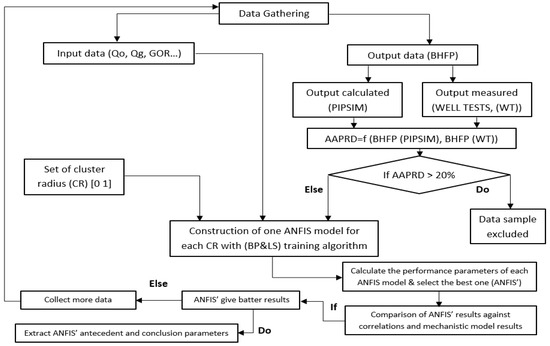
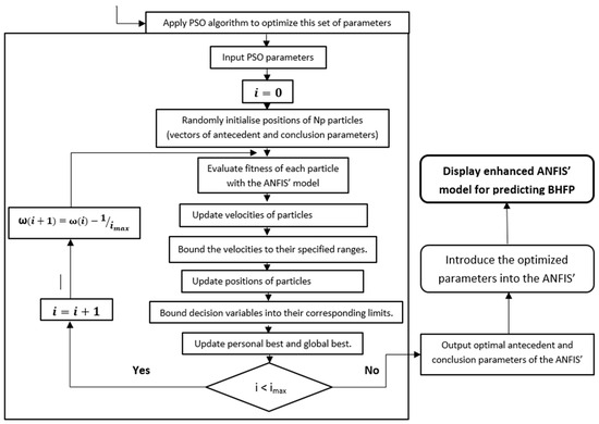
Figure 2.
Flowchart of the proposed methodology.
3.1. Data Acquisition
Data acquisition and handling are the essential steps for artificial intelligence (AI) system development. Removing outliers is important before constructing the AI model. For this study, well test data from several wells were selected to cover broad ranges of flow rates, pipe sizes, depth, flowing wellhead pressures and temperature, water cuts, gas oil ratio, oil and gas gravity, and reservoir flowing pressures. A total of 150 well test data were first gathered from numerous Algerian fields.
3.2. Data Pre-Processing and Filtration
It is necessary to remove data that were found to be either inaccurate or excessive because this kind of data can degrade the model performance. Steps for data filtration:
- Use various flow correlations to calculate the bottom hole pressure BHP by feeding well test data sets into the PIPESIM software 2020 platform.
- Calculate the AAPRE% for each correlation.
- For each data set and for all correlations, the arithmetic average of AAPRE% was computed.
- Data sets for which AAPRE% is more than 20% were removed.
After the filtration process, the ANFIS model uses 120 data sets for the development. They were divided into two parts: The model is trained using 85 data sets in the first part, and the learned ANFIS model is tested using 35 data sets in the second part.
A summary of the data parameters ranges used to build the model was shown in Table 1.

Table 1.
Data ranges for input and output variables.
3.3. ANFIS Model Development
MATLAB 2022 was used to develop the ANFIS model. The Sugeno-type FIS method was chosen because it offers a more compact and computationally efficient rule representation. It also yielded better performance compared to the popular Mamdani approach, which relies on fuzzy output sets and requires defuzzification, making it less efficient for numerical optimization tasks [35].
For designing the ANFIS model, the subtractive clustering (SC) algorithm was employed to create a Sugeno-type FIS structure for training the ANFIS. This method has the advantage over other existing methods in that it is a non-iterative algorithm which improves the cost of resolution. This technique is used to subdivide the data into several clusters where for each cluster it defines a radius of influence with values ranging from zero to one. Every data point was regarded as a possible cluster center using the subtractive clustering algorithm which also estimates the likelihood of becoming a center according to the number of nearby points [36]. When there is just a single output, the MATLAB function genfis2, which is based on the subtractive clustering algorithm, is used to generate an initial FIS (parameter initialization of the membership function) for training the ANFIS. To do this, a set of rules that model the behavior of the data is extracted. Specifically, the number of rules and antecedent membership functions were defined using the subtractive clustering method, and the consequent equations for each rule were determined using the linear least squares estimation approach. An FIS structure encompassing a collection of fuzzy rules to cover the feature space is produced by this function. Thus, distinct sets of input and output data are required by genfis2 as input arguments, as well as one cluster radius of influence for this data dimension.
Finally, it is conceivable to implement and use the ANFIS structure to imitate a given training data set after obtaining the Sugeno-type FIS structure. The ANFIS accomplishes this by utilizing a hybrid learning algorithm that combines the least squares approach with the back propagation gradient descent. This approach is used to train the membership function parameters and find the parameters of the inference system.
3.4. Optimizing ANFIS by PSO Algorithm
Antecedent and conclusion parameters are the ANFIS parameters that require training.
The antecedent parameters are the coefficients of the Gaussian MFs used in this study, as shown in Equation (29):
where (ai) and (ci) represent the variance and the center of membership functions, respectively, while (bi) is commonly set to 1.
The conclusion parameters are the coefficients of linear functions for TKS-type consequent, as shown in Equation (30):
where (pi), (qi), and (ri) are the conclusion parameters.
The values of these parameters that need updating are constrained by their upper and lower limits [−20 20].
The training and updating of this large set of ANFIS parameters is typically translated into an optimization problem which requires the employment of metaheuristic search methods that are typically successful in solving this kind of complex problem. Some of the most common algorithms that belong to this category are genetic algorithms, evolutionary strategies, gray wolf optimization (GWO), PSO, and ant colony optimization.
In this research, the chosen optimization method is the particle swarm optimization (PSO) algorithm. As demonstrated in several previous studies [37,38,39,40,41], PSO has shown strong performance when applied to real-world problems, particularly in cases involving complex, nonlinear, and high-dimensional search spaces. Among various optimization techniques, PSO stands out for its simplicity, fast convergence, and ability to effectively explore global optima, making it well-suited for training intelligent models such as ANFIS. Therefore, PSO is employed in this work to train both the consequent and antecedent parameters of the ANFIS model.
During the optimization process, all model parameters are encoded into a chromosome-like structure. The organization of this structure follows a specific order:
- ➢
- First, the antecedent parameters are placed at the beginning of the chromosome.
- ➢
- The membership function parameters of each input variable are placed in the first two genes, followed by the next two genes for the second membership function, and so on.
- ➢
- This sequence continues input-by-input until all antecedent parameters have been encoded.
- ➢
- Next, the consequent parameters (i.e., the linear coefficients of the Sugeno-type rules) are appended to the same chromosome, following the antecedent parameters.
The initial population of particles (chromosomes) is randomly generated within predefined parameter bounds. The PSO algorithm is then applied to update these particles iteratively. The fitness function used to evaluate each candidate solution is the root mean squared error (RMSE) between the predicted and actual bottom-hole pressure values on the training set. The objective is to minimize this RMSE by iteratively adjusting the parameter values within each particle until convergence is achieved.
4. Results and Discussion
After testing several clusters radii, the results obtained are provided in Table 2. It shows that the ANFIS model with a cluster radius of 0.9 could predict the bottom-hole pressure with an average absolute percentage relative deviation of 4.967% for training and 6.806% for testing. Figure 3 shows that the cluster radius of 0.9 is the best one.
Table 2.
Performance data of the ANFIS for different cluster radii.
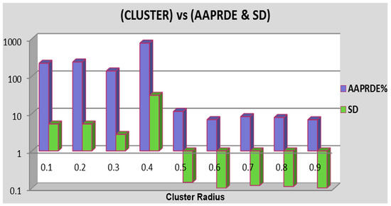
Figure 3.
Error (AAPRD%) and standard deviation for testing data for several cluster radius.
To identify the accuracy and validation of the existing models we present the following plots:
- ▪
- Cross plot (Figure 4 and Figure 5): These figures display the BHP obtained with the advanced model as opposed to experimental data. Figure 4 shows the alignment of the plotted data to the 45° straight line which is logical because the training sets of data have been firstly used for developing the ANFIS, so with a coefficient of correlation R2 of 0.997 for this set of training data, we can prove the good fitting of the data by the ANFIS. Figure 5 displays the quality of the developed model in calculating BHP with testing data. By plotting the ANFIS model results obtained for the testing data set against the actual data, and with a coefficient of correlation R2 of 0.997, we can demonstrate the accuracy of the ANFIS.
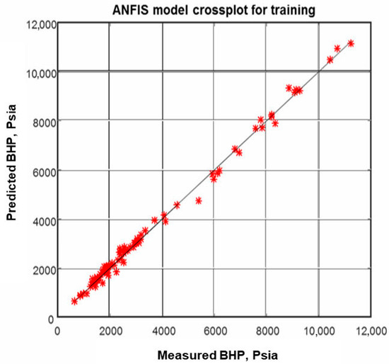 Figure 4. ANFIS model crossplot for training. The blue stars represent the predicted BHP values versus the measured BHP values, while the black line represents the perfect correlation line.
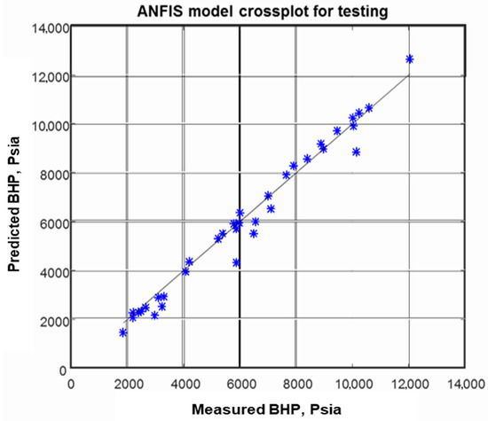 Figure 5. ANFIS model crossplot for testing. The blue stars represent the predicted BHP values versus the measured BHP values, while the black line represents the perfect correlation line.
 - ▪
- Plots of predicted vs. measured BHP (Figure 6 and Figure 7) for training and testing samples: These plots help in easily identifying the deviation of the model in predicting the BHP. Figure 6 and Figure 7 show that the ANFIS model can accurately predict the BHP for both the training and testing data sets.
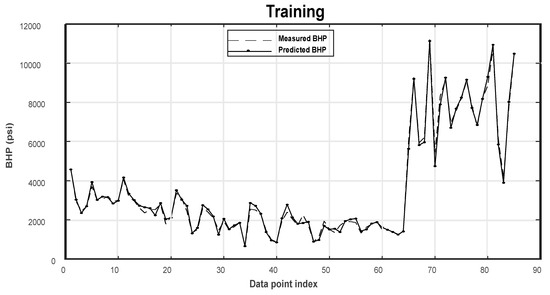 Figure 6. Results of the ANFIS for the training data sets.
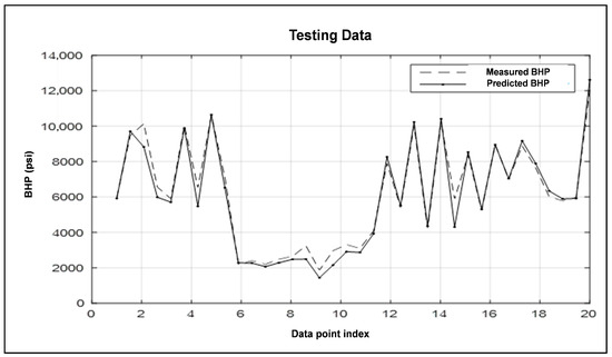 Figure 7. Results of the ANFIS for the testing data.
4.1. Comparison of the ANFIS Model Against Correlations
The ANFIS model developed earlier was implemented on the testing data and the obtained results of this model were compared to the popular approach models in the industry including Duns and Ros; Hagedorn and Brown; Aziz et al.; Ansari et al.; Mukherjee and Brill; Beggs and Brill; Orkiszewski; and Gray. Table 3 reports the values of AAPRD%, SD, and R2 for the predicted and measured BHP, evaluated by the ANFIS, empirical correlations, and mechanistic models. From this table, it is clear that the ANFIS model is able to estimate the flowing BHP with better accuracy than all the flow empirical and semi-empirical correlations covered in the study. The AAPRD and standard deviation are very low, at 6.80% and 10.19%, respectively, while the deterministic factor R2 is the highest value at 0.988. Figure 8 shows the performance comparison between all the correlations included in this study and the ANFIS. The findings in Table 3 and Figure 8 demonstrate that the ANFIS model yields more precise BHP predictions than the alternative methods considered.
Table 3.
Performance results for the ANFIS model and the other approaches.
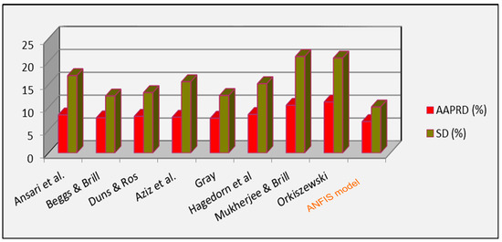
Figure 8.
AAPRD and SD comparison between the ANFIS and the other methods [16,17,18,19,20,21,22,23] to predict BHP.
4.2. Comparison of the Particle Swarm Optimization (PSO) Against the Back Propagation (BP) for ANFIS Training
The outcomes of ANFIS training using the particle swarm optimization (PSO) and back propagation (BP) algorithms are covered in this section. The ANFIS model with the PSO algorithm for learning was stable, as demonstrated by the convergence curve of error during the training process (Figure 9). Also, this method was capable of modeling the BHP with high precision. The AAPRD and the root mean square error on the testing data were 6.6495% and 477.7693, respectively. Figure 10 and Figure 11 show excellent fitting between the training and testing calculations and the real data. A performance comparison between the two algorithms (using PSO and the hybrid BP–least squares approach) for training the ANFIS to predict the BHP is presented in Table 4. This comparison shows that the PSO algorithm improves the accuracy of the ANFIS and gives better results than the basic hybrid algorithm.
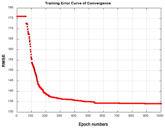
Figure 9.
Convergence curve of the error index during training. The red line represents the variation of RMSE with epoch number during training.
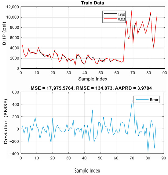
Figure 10.
Results of ANFIS hybridized with PSO for training data.
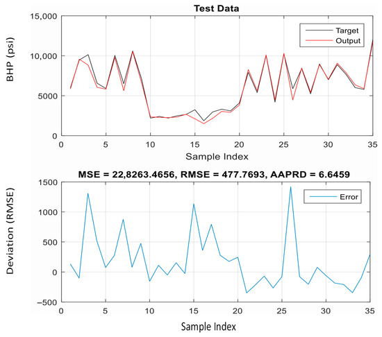
Figure 11.
Results of ANFIS hybridized with PSO for test data.
Table 4.
Performance comparison between PSO and BP-LS learning algorithms.
5. Conclusions
In this work, subtractive clustering with a cluster radius of 0.9 was used to create an Adaptive Neuro-Fuzzy Inference System (ANFIS) to estimate bottom-hole flowing pressure in multiphase flow with numerous variables and complex relationships. The predicted values of the ANFIS based on the hybrid learning algorithm have been assessed against measured BHP data obtained from the field and compared with those of the existing correlations. The results show that ANFIS could predict with the least errors (AAPRD and SD) and highest correlation coefficient compared to all empirical correlations and mechanistic models tested in this research. The ANFIS was then trained using a PSO method, and the outcomes demonstrate that the PSO approach enhances the accuracy of the ANFIS and gives better results than the basic hybrid BP-LS algorithm. Thus, hybrid computational intelligence models can be utilized to precisely determine the bottom-hole flowing pressure. Additionally, if there is no data redundancy and if more data was gathered, this new approach may perform even better. Despite the promising results, the proposed hybrid PSO–ANFIS model has several limitations. One key limitation is the limited size and diversity of the training data set, which may restrict the model’s generalizability to broader operational scenarios. In addition, the model is trained strictly within the bounds of the available input data, and as such, it lacks extrapolation capability. Therefore, special caution should be exercised when applying the model to input conditions that are not inside the training data’s range.
Future improvements to the study method described in this paper include the following:
- ➢
- Even though the system has proven effective for vertical wells with multiphase flow, it would be interesting to test the solution application to other assets such as horizontal wells, multilateral wells, and injection wells.
- ➢
- Additional heuristic and gradient-based search algorithms should be explored to enhance the efficiency of training and updating ANFIS parameters.
- ➢
- In order to enable more reliable improvement for the developed model, a larger and diverse training data set should be gathered to cover more scenarios beyond the ranges of data used in this work.
Author Contributions
Conceptualization, K.R. and A.J.G.; methodology, K.R. and A.J.G.; software, K.R.; validation, K.R. and A.J.G.; formal analysis, K.R.; investigation, K.R.; resources, K.R.; data curation, K.R.; writing—original draft preparation, K.R. and A.J.G.; writing—review and editing, K.R. and A.J.G.; visualization, K.R.; supervision, A.J.G.; project administration, A.J.G.; funding acquisition, K.R. and A.J.G. All authors have read and agreed to the published version of the manuscript.
Funding
The authors acknowledge the funding provided by the European Research Executive Agency, program HORIZON TMA Marie Sklodowska-Curie Actions MSCA Postdoctoral Fellowships—European Fellowships, under grant agreement number 101111369.
Data Availability Statement
All source code and data are available under request.
Acknowledgments
The authors acknowledge the support and resources provided by the Algerian National Oil Company SONATRACH and the university of M’Hamed Bougara of Boumerdes, which facilitated the research process and contributed to the overall success of this work.
Conflicts of Interest
The authors declare no conflicts of interest.
Nomenclature
| BHP | Bottom-hole pressure |
| AAPRD | Average absolute percentage relative deviation |
| FIS | Fuzzy Inference System |
| GOR | Gas–oil ratio |
| SD | Standard deviation |
| PSO | Particle Swarm Optimization |
| BP | Back Propagation |
| RMSE | Root Mean Square Error |
References
- Ternyik, J.; Bilgesu, H.I.; Mohaghegh, S. Virtual Measurements in Pipes: Part 1-Flowing Bottom Hole Pressure Under Multi-Phase Flow and Inclined Wellbore Conditions; SPE: Bellingham, WA, USA, 1995; p. SPE-30975. [Google Scholar]
- Takacs, G. Considerations on the Selection of an Optimum Vertical Multiphase Pressure Drop Prediction Model for Oil Wells; SPE: Tulsa, OK, USA, 2001; p. SPE-68361. [Google Scholar]
- Al-Shammari, A. Accurate Prediction of Pressure Drop in Two-Phase Vertical Flow Systems Using Artificial Intelligence; SPE: Al-Khobar, Saudi Arabia, 2011; p. SPE-149035. [Google Scholar]
- Osman, E.A.; Ayoub, M.A.; Aggour, M.A. Artificial Neural Network Model for Predicting Bottomhole Flowing Pressure in Vertical Multiphase Flow; SPE: Awali, Bahrain, 2005; p. SPE-93632. [Google Scholar]
- Barrufet, M.A.; Rasool, A.; Aggour, M.A. Prediction of Bottomhole Flowing Pressures in Multiphase Systems Using a Thermodynamic Equation of State; SPE: Tulsa, OK, USA, 1995. [Google Scholar]
- Mohammadpoor, M.; Shahbazi, K.H.; Torabi, F.; Qazvini, A. A New Methodology for Prediction of Bottomhole Flowing Pressure in Vertical Multiphase Flow in Iranian Oil fields Using Artificial Neural Networks (ANNs); SPE: Lima, Peru, 2010; p. SPE-139147. [Google Scholar]
- Wu, C.L.; Chau, K.W.; Li, Y.S. Methods to improve neural network performance in daily flows prediction. J. Hydrol. 2009, 372, 80–93. [Google Scholar] [CrossRef]
- Wang, W.C.; Chau, K.W.; Xu, D.M.; Chen, X.Y. Improving forecasting accuracy of annual runoff time series using ARIMA based on EEMD decomposition. Water Resour. Manag. 2015, 29, 2655–2675. [Google Scholar] [CrossRef]
- Zhang, S.W.; Chau, K.W. Dimension Reduction Using Semi-Supervised Locally Linear Embedding for Plant Leaf Classification. In Emerging Intelligent Computing Technology and Applications. ICIC 2009; Lecture Notes in Computer Science; Springer: Berlin/Heidelberg, Germany, 2009; Volume 5754, pp. 948–955. [Google Scholar]
- Chau, K.W.; Wu, C.L. A Hybrid Model Coupled with Singular Spectrum Analysis for Daily Rainfall Prediction. J. Hydroinform. 2010, 12, 458–473. [Google Scholar] [CrossRef]
- Zhu, Z.; Song, X.; Zhang, R.; Li, G.; Han, L.; Hu, X.; Li, D.; Yang, D.; Qin, F. A hybrid neural network model for predicting bottomhole pressure in managed pressure drilling. Appl. Sci. 2022, 12, 6728. [Google Scholar] [CrossRef]
- Agwu, O.E.; Alatefi, S.; Alkouh, A.; Suppiah, R.R. Modelling the flowing bottom hole pressure of oil and gas wells using multivariate adaptive regression splines. J. Pet. Explor. Prod. Technol. 2025, 15, 22. [Google Scholar] [CrossRef]
- Sun, H.; Luo, Q.; Xia, Z.; Li, Y.; Yu, Y. Bottomhole pressure prediction of carbonate reservoirs using XGBoost. Processes 2024, 12, 125. [Google Scholar] [CrossRef]
- Nwanwe, C.C.; Duru, U.I.; Anyadiegwu, C.; Ekejuba, A.I.B. An artificial neural network visible mathematical model for real-time prediction of multiphase flowing bottom-hole pressure in wellbores. Pet. Res. 2023, 8, 370–385. [Google Scholar] [CrossRef]
- Afagwu, C.C.; Glatz, G. Development of a hybrid modelling approach for estimating bottom hole pressure in shale and tight sand wells using smart production data and machine learning techniques. In Proceedings of the International Petroleum Technology Conference, Dhahran, Saudi Arabia, 12–14 February 2024. [Google Scholar] [CrossRef]
- Hagedorn, A.R.; Brown, K.E. Experimental Study of Pressure Gradients Occurring During Continuous Two-Phase Flow in Small-Diameter Vertical Conduits. J. Pet. Technol. 1965, 234, 475–484. [Google Scholar] [CrossRef]
- Duns, H.; Ros, N.C.J. Vertical Flow of Gas and Liquid Mixtures from Boreholes. In Proceedings of the 6th World Petroleum Congress, Frankfurt am Main, Germany, 19–26 June 1963. [Google Scholar]
- Orkiszwiski, J. Predicting Two-Phase Pressure Drops in Vertical Pipes; SPE: Bellingham, WA, USA, 1966; p. SPE-1546. [Google Scholar]
- Beggs, H.D.; Brill, J.P. A Study of Two-Phase Flow in Inclined Pipes. J. Pet. Technol. 1973, 255, 607–617. [Google Scholar] [CrossRef]
- Aziz, K.; Govier, G.W.; Fogarasi, M. Pressure Drop in Wells Producing Oil and Gas. J. Pet. Technol. 1972, 11, 38–48. [Google Scholar] [CrossRef]
- Mukhrejee, H.; Brill, J.P. Pressure Drop Correlations for Inclined Two-Phase Flow. J. Energy Resour. Technol. 1985, 107, 549–554. [Google Scholar] [CrossRef]
- Ansari, A.M.; Sylvester, N.D.; Sarica, C.; Shoham, O.; Brill, J.P. A Comprehensive Mechanistic Model for Upward Two-Phase Flow in Wellbores. SPE Prod. Facil. 1994, 9, 143–151. [Google Scholar] [CrossRef]
- Gray, H.E. Vertical Flow Correlation—Gas Wells. User Manual for API 14B, Subsurface Controlled Safety Valve Sizing Computer Program, 2nd ed.; American Petroleum Institute: Washington, DC, USA, 1978; pp. 38–41. [Google Scholar]
- Jang, J.S. ANFIS: Adaptive-Network-Based Fuzzy Inference System. IEEE Trans. Syst. Man Cybern. 1993, 23, 665–685. [Google Scholar] [CrossRef]
- Kumar, M.; Devendra, P.G. Intelligent Learning of Fuzzy Logic Controllers via Neural Network and Genetic Algorithm; USA Symposium on Flexible Automation: Seattle, WA, USA, 2004. [Google Scholar]
- Goldberg, D.E. Genetic Algorithms in Search, Optimization & Machine Learning; Addion Wesley: Reading, MA, USA, 1989. [Google Scholar]
- Kennedy, J.; Ebenhart, R.C. Particle Swarm Optimization. In Proceedings of the ICNN’95-International Conference on Neural Networks, Perth, WA, Australia, 27 November–1 November 1995; Volume 4, pp. 1942–1948. [Google Scholar]
- Rezaee Jordehi, A.; Jasni, J. Parameter selection in particle swarm optimization: A survey. J. Exp. Theor. Artif. Intell. 2013, 25, 527–542. [Google Scholar] [CrossRef]
- Rezaee Jordehi, A.; Jasni, J.; Abd Wahab, N.; Kadir, M.Z.; Javadi, M.S. Enhanced leader PSO (ELPSO): A new algorithm for allocating distributed TCSC’s in power systems. Int. J. Electr. Power Energy Syst. 2015, 64, 771–784. [Google Scholar] [CrossRef]
- Rezaee Jordehi, A.; Jasni, J. Particle swarm optimization for discrete optimization problems: A review. Artif. Intell. Rev. 2013, 43, 243–258. [Google Scholar] [CrossRef]
- Rezaee Jordehi, A. Time varying acceleration coefficients particle swarm optimization (TVACPSO): A new optimization algorithm for estimating parameters of PV cells and modules. Energy Convers. Manag. 2016, 129, 262–274. [Google Scholar] [CrossRef]
- Rezaee Jordehi, A. Particle swarm optimisation for dynamic optimisation problems: A review. Neural Comput. Appl. 2014, 25, 1507–1516. [Google Scholar] [CrossRef]
- Rezaee Jordehi, A. Particle swarm optimisation (PSO) for allocation of FACTS devices in electric transmission systems: A review. Renew. Sustain. Energy Rev. 2015, 52, 1260–1267. [Google Scholar] [CrossRef]
- Eberhart, R.; Shi, Y.; Kennedy, J. Swarm Intelligence; Morgan Kaufmann: San Mateo, CA, USA, 2001. [Google Scholar]
- Seydi Ghomsheh, V.; Aliyari Shoorehdeli, M.; Teshnehlab, M. Training ANFIS Structure with Modified PSO Algorithm. In Proceedings of the 15th Mediterranean Conference on Control & Automation, Athens, Greece, 27–29 June 2007. [Google Scholar]
- Olga, L.Q.; Alejandro, P.V.; Marcela, G.U. An approach of Anfis and Clustering Techniques to an Optimal Portfolio; Colombian Energy Market, EAFIT University: Medellín, Colombia, 2014. [Google Scholar]
- Taormina, R.; Chau, K.-W. Data-driven input variable selection for rainfall-runoff modeling using binary-coded particle swarm optimization and Extreme Learning Machines. J. Hydrol. 2015, 529, 1617–1632. [Google Scholar] [CrossRef]
- Zhang, J.; Chau, K.W. Multilayer Ensemble Pruning via Novel Multi-sub-swarm Particle Swarm Optimization. J. Univ. Comput. Sci. 2009, 15, 840–858. [Google Scholar]
- Eberhart, R.C.; Shi, Y.; Kennedy, J. Swarm Intelligence; Elsevier: Amsterdam, The Netherlands, 2001. [Google Scholar]
- Gaing, Z.L. A particle swarm optimization approach for optimum design of PID controller in AVR system. IEEE Trans. Energy Convers. 2004, 19, 384–391. [Google Scholar] [CrossRef]
- Han, W.; Yang, P.; Ren, H.; Sun, J. Comparison study of several kinds of inertia weight for PSO. In Proceedings of the IEEE International Conference on Progress in Informatics and Computing, Shanghai, China, 10–12 December 2010; IEEE Computer Society: Washington, DC, USA, 2010; pp. 280–284. [Google Scholar]


Disclaimer/Publisher’s Note: The statements, opinions and data contained in all publications are solely those of the individual author(s) and contributor(s) and not of MDPI and/or the editor(s). MDPI and/or the editor(s) disclaim responsibility for any injury to people or property resulting from any ideas, methods, instructions or products referred to in the content. |
© 2025 by the authors. Licensee MDPI, Basel, Switzerland. This article is an open access article distributed under the terms and conditions of the Creative Commons Attribution (CC BY) license (https://creativecommons.org/licenses/by/4.0/).