Modeling Local Search Metaheuristics Using Markov Decision Processes

Abstract

Local search metaheuristics like tabu search or simulated annealing are popular heuristic optimization algorithms for finding near-optimal solutions for combinatorial optimization problems. However, it is still challenging for researchers and practitioners to analyze their behavior and systematically choose one over a vast set of possible metaheuristics for the particular problem at hand. In this paper, we introduce a theoretical framework based on Markov Decision Processes (MDPs) for analyzing local search metaheuristics. This framework not only helps in providing convergence results for individual algorithms but also provides an explicit characterization of the exploration–exploitation tradeoff and a theory-grounded guidance for practitioners for choosing an appropriate metaheuristic for the problem at hand. We present this framework in detail and show how to apply it in the case of hill climbing and the simulated annealing algorithm, including computational experiments.

1. Introduction

Metaheuristics are high-level algorithmic frameworks that provide guidance or strategies for developing heuristic optimization algorithms [1]. Frequently, these strategies use concepts from other disciplines as their underlying inspiration, like the evolution process in biology, the process of cooling a metallic alloy, the cooperative behavior of flocks of birds, and many more [2]. Despite being heuristic in nature, so that in general there is no general theoretical guarantee that the algorithm will find the global optimum, metaheuristics have demonstrated a tremendous success in practice, being effectively used in applications like logistics (e.g., vehicle routing problem [3]), network design [4], scheduling [5,6,7,8], finance (e.g., portfolio optimization [9]) and many others.

In general, it can be distinguished between local search (or single-solution) metaheuristics like simulated annealing (SA) [10], tabu search (TS) [11], variable neighborhood search (VNS) [12] and large neighborhood search (LNS) [13] on the one hand, and population-based metaheuristics on the other, like genetic algorithms (GAs) [14] particle swarm optimization (PSO) [15] or estimation of distribution algorithms (EDAs) [16]. Local search metaheuristics typically start with a candidate solution $x_0$ (not necessarily feasible) and apply stochastic operators to select the next candidate solution from a suitable chosen neighborhood or pool of individuals. By iteratively repeating this process, local search metaheuristics are able to find near-optimal solutions to the problem at hand efficiently, even if the search space is very large. By contrast, population-based metaheuristics start with a group of candidate solutions (often referred to as a population) $P=\{x_1,x_2,\dots ,x_n\}$ and apply different types of operators to generate new candidate solutions, updating the population in the process.

It is well acknowledged that there is a lack of strong theoretical frameworks for understanding and analyzing the behavior of metaheuristic algorithms [17,18]. While theoretical results and convergence analysis do exist for individual algorithms like genetic algorithms and simulated annealing [19,20], existing frameworks are either focused on one type of analysis (like convergence analysis [17]), or they provide only weak results [18]. Moreover, they provide no theory-grounded guidance for practitioners on which algorithm might be most appropriate for a particular task.

In this paper, we fill this gap by proposing a novel framework based on Markov Decision Processes (MDPs) as the underlying model for metaheuristic algorithms. Specifically, in this study we focus on local search metaheuristics, leaving population-based metaheuristics for future work. We show that particular instances of local search metaheuristics can be modeled as policies of a suitably defined MDP, and based on that, we derive different coefficients to model their convergence and exploration–exploitation behavior. By introducing different parameters into these bounds and assigning them a practical meaning, we show which properties have to be taken into account for a given metaheuristic (policy) to perform well on a particular class of problems.

This paper is structured as follows. In Section 2, we review previous relevant work. Section 3 presents the MDP framework for local search metaheuristics and applies it to the hill climbing algorithm as a first example. In Section 4, we apply this framework to simulated annealing, showing how the relevant measures of convergence and exploration–exploitation can be explicitly calculated. We present some computational experiments in Section 5 that provide empirical evidence for our theoretical results. Section 6 concludes the paper and outlines future work.

2. Previous Work

Mathematical analysis of optimization metaheuristics has been done previously in the literature in a variety of ways. The work on the schema theorem by Holland [21] can be considered one of the first attempts at mathematical formalization of metaheuristic algorithms. However, this result applied only to simple GAs with one-point crossover and binary encoding. One of the most popular variants of mathematical analysis was spearheaded by the Markov chain analysis of genetic algorithms (GAs), which was mostly done in the 1990s. For instance, in early work, the authors of [22] proved that GAs with an elitist selection scheme converge to the optimum with probability 1. Suzuki [19,20] proved theoretical results based on Markov chain analysis for GAs, focusing on mutation probabilities, and developed an early comparison with simulated annealing (SA). In [23], the authors applied a non-stationary Markov model for the convergence analysis of genetic algorithms. One of the main drawbacks of using Markov chain theory for metaheuristic analysis is that Markov chains are not expressive enough for handling important aspects of the search process in metaheuristics. Critically, the reward structure and the different operators used in the algorithm can only be expressed implicitly via the transition matrix.

More recent approaches in the literature use other models, like the evolutionary Turing machine [24] and the nested partition algorithm [18]. However, most of these results focus on convergence analysis and do not handle the exploration–exploitation dilemma explicitly. This question was addressed in [25] by experimental means, but no theoretical analysis was provided. Similarly, a case study based on elitist evolutionary algorithms (concretely, random univariate search and evolutionary programming) was presented in [26] using a specially-tailored probabilistic framework. An extensive survey on the exploration–exploitation tradeoff in metaheuristics is given in [27]. In [28], a mathematical characterization of the exploration–exploitation tradeoff is given in the form of the optimal contraction theorem. However, their definition of exploration leaves out the possibility that information collected during the search can be used for exploring other areas of the search space.

In contrast to previous approaches, our framework applies Markov decision processes (MDPs) to the problem of modeling the convergence behavior and the exploration–exploitation tradeoff of local search metaheuristics. We consider MDP to be a more suitable framework than the previously presented approaches since the reward structure of the general search problem can be represented explicitly. Moreover, transformations and sequences of candidate solutions can be modeled explicitly by means of actions, which in MDP are naturally linked to rewards. We can therefore model a particular metaheuristic algorithm as a stochastic agent that makes decisions about which candidate solution to visit next based on the information obtained so far and the reward obtained. We explore the implications of this modeling choice and we show in the following sections that the convergence and the exploration–exploitation analysis of metaheuristic algorithms can be calculated explicitly.

3. Markov Decision Processes for Local Search Metaheuristics

In this section, we develop the mathematical machinery needed to define an MDP model for local search metaheuristics. Our main insight is that we can model any local search metaheuristic as a stochastic agent that executes some policy on a suitably defined MDP. Critically, we note that even if the goal of a specific metaheuristic is to find the optimum of an objective function, the algorithm itself proceeds by maximizing the total reward over a (possibly) infinite time horizon. Clearly, the rewards are directly connected with the best values found so far of the objective function, but the stochastic agent needs to proceed by gathering information about promising directions in the search space (exploration–exploitation tradeoff). Therefore, the exploration of the search space is guided mainly by the maximization of the total reward.

3.1. Definitions

We start by introducing some preliminaries in the form of notation and definitions. Then we specify the model in detail and describe how to define metaheuristic policies using this framework. In the following, we will mainly follow the conventions and definitions used in [29].

Definition 1 

(Markov Decision Process). A Markov Decision Process (MDP) is a tuple $\langle \mathcal{S},\mathcal{A},\mathcal{P},\mathcal{R},\alpha \rangle$, where:

• $\mathcal{S}$ is a set of states.
• $\mathcal{A}\left(i\right)$ is a set of actions available in state $i\in \mathcal{S}$.
• $\mathcal{P}\left(a\right)={\left\{p_{ij}\left(a\right)\right\}}_{ij}$ is the state transition matrix, given action a, where $p_{ij}\left(a\right)=\mathbb{P}\{S_{t+1}=j|S_t=i,A_t=a\}$.
• $\mathcal{R}\left(a\right)$ is a reward function, ${\mathcal{R}}_s\left(a\right)=\mathbb{E}\left[r_{t+1}\right|S_i=s,A_t=a]$.
• $\alpha \in [0,1]$ is a discount factor.

In words, an MDP is a stochastic decision model where an agent makes decisions on each time step about which action a to take from a predefined action set $\mathcal{A}\left(i\right)$, which might be different for each state $i\in \mathcal{A}\left(i\right)$. Most importantly, the transition probabilities to a new state $S_{t+1}$ depend only on the last state $S_t$ and not on the previous history (i.e., the previously visited states). This is known as the Markov property.

Definition 2. 

A policy R is a decision rule $R=({\pi }^1,{\pi }^2,\dots ,{\pi }^t,\dots )$ that can be expressed as a probability distribution of the actions, given states:

$${\pi }_{ia}^t=\mathbb{P}\{A_t=a|S_t=s\}$$

If the policy R is such that there exists an action a such that ${\pi }_{ia}^t=1$ for every state $i\in \mathcal{S}$, we say the policy is deterministic; otherwise, we call the policy stochastic. If the policy does not depend on time, we call this policy stationary and simply write ${\pi }_{ia}$.

The natural problem that now arises is how to find policies that maximize the rewards obtained in some precise sense. This is captured by means of a utility function, which might be, e.g., maximize the total expected or average reward. An MDP can be classified according to its time horizon in finite or infinite time MDP. Likewise, we can also distinguish between discrete and continuous time MDPs. For local search metaheuristics, we focus on the MDP formulation where:

• The time is discrete and the time horizon is infinite.
• The utility function is the total expected reward.

Regarding condition (1), we note that clearly the execution time of a metaheuristic is always finite, but this finite time cannot be fixed beforehand (except for the class of metaheuristics that are run for a fixed number of iterations). This is modeled by having terminal states with no outgoing transitions (i.e., the probability of transitioning to any other state is 0, and $\mathcal{A}\left(i\right)=\varnothing$ for all terminal states $i\in \mathcal{S}$). We argue for condition (2) that, in general, the main strategy used by all metaheuristics is to search for the optimum indirectly by exploring the search space $\mathcal{X}$ and exploiting promising regions where an optimum $x^{\ast }\in \mathcal{X}$ is supposed to be. However, this is done by sampling from the search space in some specific sense and evaluating the objective function f on that sample, thus collecting information about the target function value. If we interpret this sampling and evaluating procedure as collecting rewards, the agent (i.e., the metaheuristic) can be interpreted as trying to maximize the total reward obtained.

3.2. Optimal Policies

In general, we model local search metaheuristic algorithms by means of policies R as defined before. We define the reward of such a policy as the total (discounted) expected reward:

$$v_i^{\alpha }\left(R\right)=\sum _{t=1}^{\infty }{\mathbb{E}}_{i,R}\left\{{\alpha }^{t-1}{r}_t\right\}$$

(1)

where $r_t$ denotes the collected actual reward at time step t, and the expectation is over policy R, given initial state $i\in \mathcal{S}$, and $\alpha$ is a discount factor that regulates the value of future rewards. In the following, we will assume $\alpha =1$ so we can write:

$$v_i\left(R\right)=\sum _{t=1}^{\infty }\sum _{j,a}\mathbb{P}\{S_{t+1}=j|S_t=i,A_t=a\}{r}_j\left(a\right)$$

(2)

where $r_j\left(a\right)$ denotes the reward obtained from state j after action a. Let ${\left\{P\left({\pi }^t\right)\right\}}_{ij}$ denote the transition matrix of policy R, and ${\left\{r\left({\pi }^t\right)\right\}}_i$ its reward vector. We have  

$$\begin{array}{cc}\hfill {\left\{P\left({\pi }^t\right)\right\}}_{ij}& =\sum _{a\in \mathcal{A}}{p}_{ij}^t\left(a\right){\pi }_{ia}^t\mathrm{for}\mathrm{all}i,j\in \mathcal{S}\hfill \end{array}$$

(3)

$$\begin{array}{cc}\hfill {\left\{r\left({\pi }^r\right)\right\}}_i& =\sum _{a\in \mathcal{A}}{r}_i^t\left(a\right){\pi }_{ia}^t\mathrm{for}\mathrm{all}i\in \mathcal{S}\hfill \end{array}$$

(4)

The reward of policy R can be now expressed based on the transition probabilities as follows:

$$v^{\alpha }\left(R\right)=\sum _{t=1}^{\infty }{\alpha }^{t-1}P\left({\pi }^1\right)P\left({\pi }^2\right)\dots P\left({\pi }^{t-1}\right)r\left({\pi }^t\right)$$

(5)

Definition 3. 

We call a policy $R_{\ast }$ optimal if it is the best achievable policy considering the reward function, i.e.,

$$v^{\alpha }\left(R_{\ast }\right)={sup}_R{v}^{\alpha }\left(R\right)$$

3.3. Local Search Metaheuristics as Policies

We now formally represent an arbitrary local search metaheuristic as a policy in an MDP as follows. In this study, we focus on binary strings of length n as candidate solutions, therefore $\mathcal{X}\subseteq {\{0,1\}}^n$. From now on, we denote by $\mathbf{x}\in {\{0,1\}}^n$ a binary vector that is a candidate solution for the problem at hand, which might be feasible or not (i.e., it can be that, during the search process, there is an ${\mathbf{x}}_t$ such that ${\mathbf{x}}_t\notin \mathcal{X}$). In the following, we will assume (without loss of generality) a maximization problem, i.e., find ${\mathbf{x}}^{\ast }$ such that ${\mathbf{x}}^{\ast }={argmax}_{\mathbf{x}\in \mathcal{X}}f\left(\mathbf{x}\right)$.

Definition 4. 

A criterium H is a function $H:\mathcal{X}\times \mathcal{X}\to \{0,1\}$ such that $H({\mathbf{x}}^{\prime };\mathbf{x})=1$ if and only if ${\mathbf{x}}^{\prime }$ is a neighbour of $\mathbf{x}$ according to a metaheuristic-specific strategy, and 0 otherwise.

Typically, instantiations of different local search metaheuristics provide one or several criteria H to determine which candidate solutions ${\mathbf{x}}^{\prime }$ can be considered neighbors of the current solution $\mathbf{x}$. For instance, in hill-climbing there is typically only one criterium H that defines the possible candidate solutions starting from the current one (for instance, all solutions that can be obtained from the current one by flipping a random bit). However, other metaheuristics like VNS typically require a set of criteria $\mathcal{H}=\{H_1,\dots ,H_n\}$ to be specified, and the algorithm iterates in some form over $\mathcal{H}$.

Definition 5. 

We define a neighborhood ${\mathcal{N}}_H\left(\mathbf{x}\right)$ as the subset of $\mathcal{X}$ induced by H, i.e., all candidate solutions ${\mathbf{x}}^{\prime }\in \mathcal{X}$ that are neighbors of $\mathbf{x}$ according to criterium H; therefore, ${\mathcal{N}}_H\left(\mathbf{x}\right)=\{x^{\prime }\in \mathcal{X}|H({\mathbf{x}}^{\prime };\mathbf{x})=1\}$.

Let $\mathbf{x}\in \mathcal{X}$ and ${\mathbf{x}}^{\prime }\in {\mathcal{N}}_H\left(\mathbf{x}\right)$. We denote by $\mathbf{x}\mapsto {\mathbf{x}}^{\prime }$ the operator that transforms $\mathbf{x}$ into ${\mathbf{x}}^{\prime }$. For example, the neighborhood of all binary strings located at Hamming distance one from $\mathbf{x}$ would be defined by ${\mathcal{N}}_{H_D}\left(\mathbf{x}\right)=\{x^{\prime }\in \mathcal{X}|H_D({\mathbf{x}}^{\prime };\mathbf{x})=1\}$. In this case, $\mathbf{x}\mapsto {\mathbf{x}}^{\prime }$ denotes the operator that flips the one bit necessary to turn $\mathbf{x}$ into ${\mathbf{x}}^{\prime }$.

Definition 6 

(Local search MDP). Let our local search MDP be defined by:

• $\mathcal{S}=\{0,1,\dots ,2^{n-1}\}$. Any state $i\in \mathcal{S}$ can trivially be converted into a candidate solution as the binary representation of the integer i.
• $\mathcal{A}\left(i\right)=\{i\mapsto j|j\in {\bigcup }_k{\mathcal{N}}_k\}$, the set of all possible transformations in all neighborhoods applicable to the current state $i\in \mathcal{S}$.
• The transition probabilities, for all $i,j\in \mathcal{S}$, $a\in \mathcal{A}\left(i\right)$:

  $$p_{ij}\left(a\right)=\left\{\begin{array}{c}1/\left|\mathcal{A}\right(i\left)\right|,\mathit{if}a=i\mapsto j\hfill \\ 0,\mathit{otherwise}\hfill \end{array}\right.$$

  (6)
• The reward for state j given action $a=i\mapsto j$ is defined by $r_j\left(a\right)=f\left(j\right)-f\left(i\right)$, where f is the objective function (note the slight abuse of notation here since f is defined on $\mathcal{X}$ rather than $\mathcal{S}$, but the conversion is trivial).

An instantiation of this MDP therefore starts at an arbitrary state $i\in \mathcal{S}$ and visits a number of states according to the transition probabilities before halting at time T. The algorithm terminates as soon as it reaches a terminal or absorbing state, i.e., a state $i\in \mathcal{S}$ where the transition probability of reaching any other state is 0 ($p_{ij}\left(a\right)=0$ for all $i\ne j$, and $p_{ii}\left(a\right)=1$ otherwise). Note that the rewards are chosen in such a way that, in general, they incentivize making progress towards any optimum ${\mathbf{x}}^{\ast }$, setting the stage for the optimization process to advance towards an optimal solution.

In this setting, we identify a policy R with a particular local search metaheuristic.

Example 1 

(Hill climbing). We define a policy $R_{HC}$ for the standard hill climbing algorithm as follows:

• $\mathcal{A}\left(i\right)=\{i\mapsto j|j\in {\mathcal{N}}_{H_D}\}$ as defined before (we flip one bit), and
• Let $\mathcal{M}\left(i\right)=\{j\in \mathcal{S}|j=argmaxf\left(j^{\prime }\right),a=i\mapsto j,a\in \mathcal{A}\left(i\right)\}$, then

  $${\pi }_{ia}=\left\{\begin{array}{c}1/\left|\mathcal{M}\right(i\left)\right|,\mathit{if}j\in \mathcal{M}\left(i\right)\hfill \\ 0,\mathit{otherwise}\hfill \end{array}\right.$$

  (7)

Note that $R_{HC}$ is a deterministic policy except when $\left|\mathcal{M}\right(i\left)\right|>1$, in which case ties are broken randomly.

In general, the MDP formulation is defined in such a way that the balance between exploration and exploitation becomes explicit in the definition of the policy. Informally, the agent can either maximize the reward in the short run (thus going into an exploitation phase), or temporarily accept negative rewards and therefore going into an exploration phase, which will depend on the particular trajectory taken from an initial solution ${\mathbf{x}}_{\mathbf{0}}$. Using the previous notions, we define exploration and exploitation explicitly as follows:

Definition 7 

(Exploration and exploitation). Let $a\in \mathcal{A}\left(i\right)$ be an action such that $a=i\mapsto j$. We say that a is an exploration action if and only if $r_j\left(a\right)\le 0$. Otherwise, we call a an exploitation action.

Definition 8 

(Exploration–exploitation function). Let $\sigma :\mathcal{A}\left(i\right)\to \{0,1\}$ be a function such that $\sigma \left(a\right)=1$ if and only if a is an exploration action, and $\sigma \left(a\right)=0$ otherwise. We call σ the exploration–exploitation function.

We now state our main result, which shows that any local search metaheuristic can be represented by a policy where the balance between exploration and exploitation becomes explicit.

Theorem 1 

(Local search exploration-exploitation theorem). Let M be a local search MDP. For any local search metaheuristic A, there exists a policy $R_A$ such that

$${\pi }_{ia}^t={\alpha }_i^A\left(t\right)\mathbb{P}\{\sigma \left(a\right)=1|S_t=i\}+{\beta }_i^A\left(t\right)\mathbb{P}\{\sigma \left(a\right)=0|S_t=i\}$$

(8)

Theorem 1 shows that for any metaheuristic A, we can explicitly construct the corresponding policy as a mixture of exploration and exploitation actions.

Proof. 

Let ${\mathcal{M}}_t^{+}\left(i\right)=\{j\in \mathcal{S}|f\left(j\right)>f\left(i\right),a=i\mapsto j,a\in \mathcal{A}\left(i\right),S_t=i\}$ and ${\mathcal{M}}_t^{-}\left(i\right)=\{j\in \mathcal{S}|f\left(j\right)\le f\left(i\right),a=i\mapsto j,a\in \mathcal{A}\left(i\right),S_t=i\}$ be the sets of improving and non-improving states given action a, respectively. We have:

$$\begin{array}{cc}\hfill {\pi }_{ia}^t& =\mathbb{P}\{A_t=a|S_t=i\}\hfill \\ \hfill & =\mathbb{P}\{A_t=a,j\in {\mathcal{M}}_t^{+}\left(i\right)|S_t=i\}+\mathbb{P}\{A_t=a,j\in {\mathcal{M}}_t^{-}\left(i\right)|S_t=i\}\hfill \\ \hfill & ={\displaystyle \frac{|{\mathcal{M}}_t{\left(i\right)}^{+}|}{|{\mathcal{M}}_t{\left(i\right)}^{+}|+|{\mathcal{M}}_t{\left(i\right)}^{-}|}}\mathbb{P}\{\sigma \left(a\right)=0|S_t=i\}+\hfill \\ \hfill & +{\displaystyle \frac{|{\mathcal{M}}_t{\left(i\right)}^{-}|}{|{\mathcal{M}}_t{\left(i\right)}^{+}|+|{\mathcal{M}}_t{\left(i\right)}^{-}|}}\mathbb{P}\{\sigma \left(a\right)=1|S_t=i\}\hfill \end{array}$$

(9)

Therefore,

$${\alpha }_i^A\left(t\right)={\displaystyle \frac{|{\mathcal{M}}_t{\left(i\right)}^{-}|}{|{\mathcal{M}}_t{\left(i\right)}^{+}|+|{\mathcal{M}}_t{\left(i\right)}^{-}|}},\mathrm{and}{\beta }_i^A\left(t\right)={\displaystyle \frac{|{\mathcal{M}}_t{\left(i\right)}^{+}|}{|{\mathcal{M}}_t{\left(i\right)}^{+}|+|{\mathcal{M}}_t{\left(i\right)}^{-}|}}$$

   □

Theorem 1 and its proof provide hints to several measures of interest. The first one is a measure that can be used for convergence analysis and defined as follows:

$${\gamma }_i^A\left(t\right):={\displaystyle \frac{{\beta }_i^A\left(t\right)}{{\alpha }_i^A\left(t\right)}}={\displaystyle \frac{|{\mathcal{M}}_t{\left(i\right)}^{+}|}{|{\mathcal{M}}_t{\left(i\right)}^{-}|}}$$

(10)

We call ${\gamma }_i^A\left(t\right)$ the convergence coefficient of local search metaheuristic A (conditioned on initial state $i\in \mathcal{S}$) at time t, and denote ${\gamma }^A\left(t\right)$ as the vector of all ${\left\{{\gamma }_i^A\left(t\right)\right\}}_{i\in \mathcal{S}}$ (that we call convergence vector). We can now study the convergence behavior of local search metaheuristics according to the limit of the components ${\gamma }_i^A\left(t\right)$ as $t\to \infty$. For instance, if ${lim}_{t\to \infty }{\gamma }_i^A\left(t\right)=0$ (for some state i), this means that algorithm A has converged, since the improving set becomes zero faster than the non-improving set. Note that ${\gamma }_i^A\left(t\right)=0$ only implies convergence and not optimality (i.e., it can be a local optimum).

The second relevant measure represents an explicit way of evaluating the balance between exploration and exploitation that a specific local search metaheuristic provides. We define

$${\delta }_{ia}^A\left(t\right):={\displaystyle \frac{\mathbb{P}\{\sigma \left(a\right)=1|S_t=i\}}{\mathbb{P}\{\sigma \left(a\right)=0|S_t=i\}}}$$

(11)

Averaging over all actions, we get

$${\delta }_i^A=\sum _{t=0}^{\infty }{\delta }_i^A\left(t\right)={\sum }_{t=0}^{\infty }{\sum }_{j\in \mathcal{A}\left(i\right)}{p}_{ij}\left(a\right){\delta }_{ja}^A\left(t\right)={\displaystyle \frac{1}{\left|\mathcal{A}\right(i\left)\right|}}\sum _{j\in \mathcal{A}\left(i\right)}\sum _{t=0}^{\infty }{\delta }_{ja}^A\left(t\right)$$

(12)

We call ${\delta }_i^A$ the exploration–exploitation coefficient of local search metaheuristic A conditioned on initial state $i\in \mathcal{S}$. In vector notation, we write ${\delta }^A$ and call it the exploration–exploitation coefficient vector. In general, there can be components of ${\delta }^A$ that converge and others that diverge. Therefore, one possibility would be to assert the general exploration–exploitation behavior of A based on ${\delta }_{\ast }^A={max}_i{\delta }_i^A$ and investigate the individual components of ${\delta }^A$ in case a more detailed analysis is needed.

We can now define for each metaheuristic a measure of its exploration–exploitation balance as follows:

Definition 9. 

We say that A is a balanced local search metaheuristic if ${\delta }_{\ast }^A=C$ for a constant $C>0,C\in \mathbb{R}$. Otherwise, if ${\delta }_{\ast }^A$ diverges to ∞, we say that A is exploration-oriented. Finally, if ${\delta }_{\ast }^A=0$, we say that A is exploitation-oriented.

Using our local search MDP, we have transformed the problem of convergence analysis and determining the exploration–exploitation balance of any metaheuristic into the quantitative problem of calculating ${\delta }_i^A$, ${\delta }_{\ast }^A$ and the limits of ${\gamma }_i^A\left(t\right)$ as $t\to \infty$ for $i\in \mathcal{S}$. We now apply these notions to the hill climbing heuristic already mentioned before.

Example 2. 

In the case of hill climbing, for every $i\in \mathcal{S}$ we have:

$$\begin{array}{cc}\hfill {\alpha }_i^A\left(t\right)& =0\hfill \\ \hfill {\beta }_i^A\left(t\right)& =1/\left|\mathcal{M}\right(i\left)\right|\hfill \\ \hfill {\gamma }_i^A\left(t\right)& =0\hfill \end{array}$$

(13)

Since ${lim}_{t\to \infty }{\gamma }_i^A\left(t\right)=0,\forall i\in \mathcal{S}$, we have that hill climbing always converges to a (possibly local) optimum. Regarding exploration–exploitation behavior, we have ${\delta }_{ia}\left(t\right)=0,\forall a\in \mathcal{A}\left(i\right),\forall i\in \mathcal{S}$. We therefore obtain that ${\delta }_{\ast }^A=0$ and hill climbing is exploitation-oriented.

3.4. Summary

For the sake of clarity, we provide a graphical summary of our approach in Figure 1. In this figure, we depict the analysis described in the text as a sequence of five steps and break down each step according to the measures defined.

In the next section, we apply our MDP model to the simulated annealing (SA) metaheuristic and derive some of its convergence and exploration–exploitation properties.

4. Simulated Annealing

Simulated annealing (SA) [10] is a local search metaheuristic inspired by the procedure of cooling a molten solid according to a predefined schedule. The main idea is to start with a high temperature T and decrease this temperature in subsequent iterations with the goal of reaching the minimum value of an energy function E. Transitions from the current candidate solution that improve the objective value are accepted with probability 1. Otherwise, the solution is accepted with a probability that depends on the magnitude of the difference between the current best objective value and the value of the new candidate solution. In the initial, high-temperature phase, the probability of accepting worse solutions is high (emphasizes exploration), whereas in later stages lower temperatures also decrease this probability (emphasizes exploitation). More formally, this probability can be written as:

$$\mathbb{P}\{{\mathbf{x}}_{t+1}={\mathbf{x}}^{\prime }|{\mathbf{x}}_t=\mathbf{x}\}=\left\{\begin{array}{c}1,\mathrm{if}E\left({\mathbf{x}}^{\prime }\right)<E\left(\mathbf{x}\right)\hfill \\ exp\left({\displaystyle \frac{-\left(E\left(\mathbf{x}\right)-E\left({\mathbf{x}}^{\prime }\right)\right)}{T}}\right),\mathrm{otherwise}\hfill \end{array}\right.$$

(14)

In our case, since we are solving by convention maximization problems, without loss of generality we set $E=-f$. Usually, a geometric cooling scheme is used: $T_{new}=\alpha T_{current}$, where $\alpha \in [0,1)$. Let $T_0$ denote the initial temperature (which is a free parameter of the algorithm). Then the temperature at time t is given by $T={\alpha }^t{T}_0$.

We now define a policy $R_{SA}$ to model the behavior of SA as a stochastic decision agent as follows:

• Let ${\mathcal{M}}_t^{+}\left(i\right)$ and ${\mathcal{M}}_t^{-}\left(i\right)$ be defined as in Theorem 1.
• Let us consider action $a=i\mapsto j$ and state $i\in \mathcal{S}$. Using Theorem 1 we obtain

  $$\begin{array}{cc}\hfill {\pi }_{ia}^t& =\mathbb{P}\{A_t=a|S_t=i\}\hfill \\ \hfill & ={\displaystyle \frac{|{\mathcal{M}}_t{\left(i\right)}^{+}|}{|{\mathcal{M}}_t{\left(i\right)}^{+}|+|{\mathcal{M}}_t{\left(i\right)}^{-}|}}+{\displaystyle \frac{|{\mathcal{M}}_t{\left(i\right)}^{-}|}{|{\mathcal{M}}_t{\left(i\right)}^{+}|+|{\mathcal{M}}_t{\left(i\right)}^{-}|}}exp\left(-{\displaystyle \frac{f\left(j\right)-f\left(i\right)}{{\alpha }^t{T}_0}}\right)\hfill \end{array}$$

  (15)

Now, the convergence coefficients can be calculated as follows:

$$\underset{t\to \infty }{lim}{\gamma }_i^A\left(t\right)=\underset{t\to \infty }{lim}{\displaystyle \frac{|{\mathcal{M}}_t{\left(i\right)}^{+}|}{|{\mathcal{M}}_t{\left(i\right)}^{-}|}}\underset{t\to \infty }{\to }0,\forall i\in \mathcal{S}$$

(16)

Since when time approaches infinity, assuming a geometric cooling scheme, the algorithm will only accept improving actions and in the limit there will be more non-improving than improving actions (note that $\alpha <1$ by definition).

Let us now calculate the exploration–exploitation coefficient:

$$\mathbb{P}\{\sigma \left(a\right)=1|S_t=i\}=\left\{\begin{array}{cc}0,\hfill & \mathrm{if}f\left(j\right)>f\left(i\right)\hfill \\ exp\left(-{\displaystyle \frac{f\left(j\right)-f\left(i\right)}{{\alpha }^t{T}_0}}\right),\hfill & \mathrm{otherwise}\hfill \end{array}\right.$$

(17)

Using Equations (11) and (12) we get:

$${\delta }_i^A={\displaystyle \frac{1}{\left|\mathcal{A}\right(i\left)\right|}}\sum _{j\in \mathcal{A}\left(i\right)}\sum _{t=0}^{\infty }{\delta }_{ja}^A\left(t\right)={\displaystyle \frac{1}{\left|\mathcal{A}\right(i\left)\right|}}\sum _{\begin{array}{c}j\in \mathcal{A}\left(i\right)\\ f\left(j\right)\ge f\left(i\right)\end{array}}\sum _{t=0}^{\infty }exp\left(-{\displaystyle \frac{f\left(j\right)-f\left(i\right)}{{\alpha }^t{T}_0}}\right)$$

(18)

which for all $i\in \mathcal{S}$ and $\alpha \in [0,1)$ converges to a positive constant $C>0$, since:

$${\displaystyle \frac{exp\left(-\frac{f\left(j\right)-f\left(i\right)}{{\alpha }^{t+1}{T}_0}\right)}{exp\left(-\frac{f\left(j\right)-f\left(i\right)}{{\alpha }^t{T}_0}\right)}}=exp\left(-{\displaystyle \frac{(1-\alpha )\left(f\right(j)-f(i\left)\right)}{{\alpha }^{t+1}{T}_0}}\right)\underset{t\to \infty }{\to }0$$

(19)

Therefore, simulated annealing is a balanced local search metaheuristic according to our definition.

5. Computational Experiments

In this section, we present some preliminary computational experiments (the code for the experiments is publicly available under https://github.com/IMC-UAS-Krems/mdp_local_search_experiments, accessed on 12 August 2025) that validate the theoretical results obtained in the previous section. We calculate the convergence and exploration–exploitation coefficients ${\gamma }^A\left(t\right)$ and ${\delta }^A\left(t\right)$ explicitly for hill climbing and simulated annealing and visualize their temporal evolution using a random initial state across sample runs with the OneMax problem. In OneMax, the objective is to maximize the number of 1’s of an n bit string, starting from a randomly generated solution. It represents a widely used and simple benchmark for preliminary tests applied to search heuristics.

5.1. Hill Climbing

Figure 2 shows a visualization of the temporal evolution of the convergence coefficient across a sample run of the algorithm using $n=30$ as string size. As can be seen, the convergence coefficient decreases monotonically until it reaches 0 on the last iteration (red curve) as theoretically predicted. Since there is always an increment of 1 in the objective function after each move, the objective function also increases monotonically and linearly until reaching the optimal objective value (blue curve).

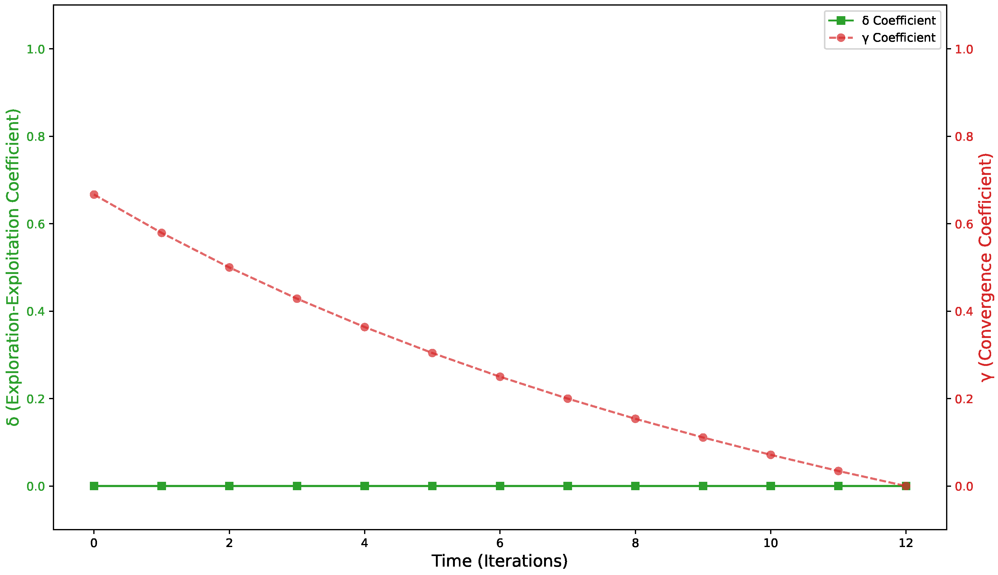
In Figure 3, we plot the evolution of both the convergence and the exploration–exploitation coefficient in another run of hill climbing (starting from a new random string). As can be seen, the exploration–exploitation coefficient stays (by definition) at 0, indicating that only exploitation-oriented moves, and no exploration-oriented, are performed by the algorithm.

5.2. Simulated Annealing

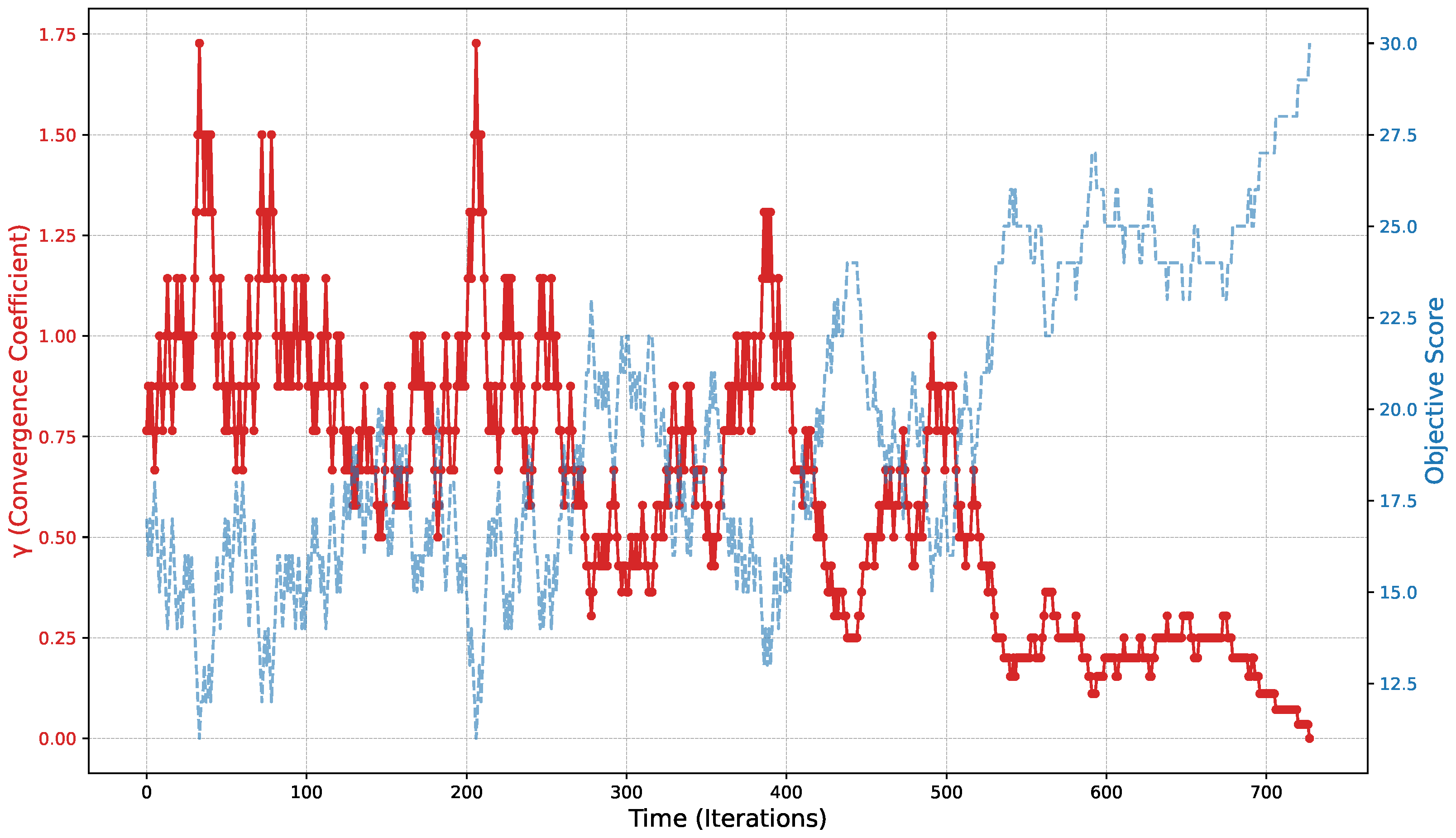
In the case of SA, we provide the evolution of the convergence coefficient in Figure 4. In this case, the evolution of both ${\gamma }^A$ and the objective value differ substantially from hill climbing. In the initial stages of the algorithm (where T is still high), ${\gamma }^A$ fluctuates as expected, alternating between improving and non-improving moves. However, as the temperature decreases and the algorithm focuses on promising regions of the search space, the fluctuations are also reduced and ${\gamma }^A$ reaches its final value of 0, indicating that the algorithm has converged.

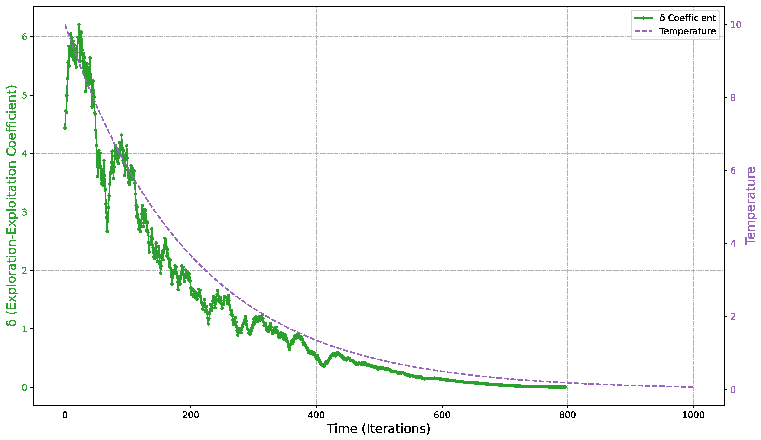
Figure 5 provides a visualization of the evolution of the exploration–exploitation coefficient for SA. As expected from the theoretical discussion, the evolution of the coefficient closely matches the current temperature: in the initial stages (high temperature), ${\delta }^A$ is also high, while in later stages with decreasing temperature, the coefficient also decreases, signaling the transition from a highly exploration-oriented to exploitation-oriented behavior. In sum, we can conclude that SA has a balanced exploration–exploitation behavior.

6. Conclusions

In this paper, we have presented a new framework for modeling the convergence and exploration–exploitation behavior of local search metaheuristics based on Markov decision processes. This framework provides a novel and intuitive way of characterizing essential properties of local search metaheuristics in a principled way. We proved that any local search metaheuristic can be analyzed using the tools provided and showed how to apply the framework in two cases: the hill climbing and the simulated annealing metaheuristics. In the case of hill climbing, we showed that the framework correctly classifies it as exploitation-oriented, whereas simulated annealing was classified as balanced, which is consistent with the general consensus in the literature. Our study goes beyond the state-of-the-art in metaheuristic analysis, since the tools we develop provide a more expressive methodology than methods based on Markov chains and other probabilistic approaches. As a consequence, the behavior of local search metaheuristics can be modeled in a more realistic way and the results obtained are consistent with practice.

As future work, we plan to extend our results to other local search metaheuristics like variable neighborhood search (VNS) [12] and large neighborhood search (LNS) [30]. Additionally, the framework will be extended to be able to handle population-based metaheuristics (PBMHs) like genetic algorithms (GA) [14], particle swarm optimization (PSO) [15] and estimation of distribution algorithms (EDAs) [16]. Additionally, more empirical studies will be conducted with the goal of explicitly calculating the measures described in this paper for different stages in the optimization process and different instances, potentially leading to new tools for instance space analysis.

References

1. Sörensen, K.; Glover, F. Metaheuristics. In Encyclopedia of Operations Research and Management Science; Springer: Boston, MA, USA, 2013; Volume 62, pp. 960–970. [Google Scholar]
2. Silberholz, J.; Golden, B. Comparison of Metaheuristics. In Handbook of Metaheuristics; Gendreau, M., Potvin, J.Y., Eds.; Springer: Boston, MA, USA, 2010; pp. 625–640. [Google Scholar] [CrossRef]
3. Lin, S.W.; Lee, Z.J.; Ying, K.C.; Lee, C.Y. Applying hybrid meta-heuristics for capacitated vehicle routing problem. Expert Syst. Appl. 2009, 36, 1505–1512. [Google Scholar] [CrossRef]
4. Fernandez, S.A.; Juan, A.A.; de Armas Adrián, J.; Silva, D.G.e.; Terrén, D.R. Metaheuristics in Telecommunication Systems: Network Design, Routing, and Allocation Problems. IEEE Syst. J. 2018, 12, 3948–3957. [Google Scholar] [CrossRef]
5. Pillay, N. A survey of school timetabling research. Ann. Oper. Res. 2014, 218, 261–293. [Google Scholar] [CrossRef]
6. Kaur, M.; Saini, S. A Review of Metaheuristic Techniques for Solving University Course Timetabling Problem. In Advances in Information Communication Technology and Computing; Goar, V., Kuri, M., Kumar, R., Senjyu, T., Eds.; Lecture Notes in Networks and Systems; Springer: Singapore, 2021; pp. 19–25. [Google Scholar] [CrossRef]
7. Ecoretti, A.; Ceschia, S.; Schaerf, A. Local search for integrated predictive maintenance and scheduling in flow-shop. In Proceedings of the 14th Metaheuristics International Conference, Syracuse, Italy, 11–14 July 2022. [Google Scholar]
8. Ceschia, S.; Guido, R.; Schaerf, A. Solving the static INRC-II nurse rostering problem by simulated annealing based on large neighborhoods. Ann. Oper. Res. 2020, 288, 95–113. [Google Scholar] [CrossRef]
9. Doering, J.; Kizys, R.; Juan, A.A.; Fitó, À.; Polat, O. Metaheuristics for rich portfolio optimisation and risk management: Current state and future trends. Oper. Res. Perspect. 2019, 6, 100121. [Google Scholar] [CrossRef]
10. Kirkpatrick, S.; Gelatt, C.D., Jr.; Vecchi, M.P. Optimization by simulated annealing. Science 1983, 220, 671–680. [Google Scholar] [CrossRef] [PubMed]
11. Glover, F.; Laguna, M. Tabu Search; Springer: Berlin/Heidelberg, Germany, 1998. [Google Scholar]
12. Mladenović, N.; Hansen, P. Variable neighborhood search. Comput. Oper. Res. 1997, 24, 1097–1100. [Google Scholar] [CrossRef]
13. Shaw, P. Using constraint programming and local search methods to solve vehicle routing problems. In Proceedings of the International Conference on Principles and Practice of Constraint Programming, Pisa, Italy, 26–30 October 1998; pp. 417–431. [Google Scholar]
14. Holland, J.H. Genetic Algorithms. Sci. Am. 1992, 267, 66–73. [Google Scholar] [CrossRef]
15. Kennedy, J.; Eberhart, R. Particle swarm optimization. In Proceedings of the ICNN’95—International Conference on Neural Networks, Perth, WA, Australia, 27 November–1 December 1995; Volume 4, pp. 1942–1948. [Google Scholar]
16. Larrañaga, P.; Lozano, J.A. Estimation of Distribution Algorithms: A New Tool for Evolutionary Computation; Springer Science & Business Media: Berlin, Germany, 2001; Volume 2. [Google Scholar]
17. Liu, B.; Wang, L.; Liu, Y.; Wang, S. A unified framework for population-based metaheuristics. Ann. Oper. Res. 2011, 186, 231–262. [Google Scholar] [CrossRef]
18. Chauhdry, M.H.M. A framework using nested partitions algorithm for convergence analysis of population distribution-based methods. EURO J. Comput. Optim. 2023, 11, 100067. [Google Scholar] [CrossRef]
19. Suzuki, J. A Markov chain analysis on simple genetic algorithms. IEEE Trans. Syst. Man Cybern. 1995, 25, 655–659. [Google Scholar] [CrossRef]
20. Suzuki, J. A further result on the Markov chain model of genetic algorithms and its application to a simulated annealing-like strategy. IEEE Trans. Syst. Man Cybern. Part B (Cybern.) 1998, 28, 95–102. [Google Scholar] [CrossRef] [PubMed]
21. Holland, J.H. Adaptation in Natural and Artificial Systems: An Introductory Analysis with Applications to Biology, Control, and Artificial Intelligence; U Michigan Press: Ann Arbor, MI, USA, 1975. [Google Scholar]
22. Eiben, A.E.; Aarts, E.H.L.; Van Hee, K.M. Global convergence of genetic algorithms: A markov chain analysis. In Proceedings of the Parallel Problem Solving from Nature, Dortmund, Germany, 1–3 October 1991; Schwefel, H.P., Männer, R., Eds.; Springer: Berlin/Heidelberg, Germany, 1991; pp. 3–12. [Google Scholar] [CrossRef]
23. Cao, Y.; Wu, Q. Convergence analysis of adaptive genetic algorithms. In Proceedings of the Second International Conference on Genetic Algorithms in Engineering Systems: Innovations and Applications, Glasgow, UK, 2–4 September 1997; pp. 85–89, ISSN 0537-9989. [Google Scholar] [CrossRef]
24. Eberbach, E. Toward a theory of evolutionary computation. Biosystems 2005, 82, 1–19. [Google Scholar] [CrossRef] [PubMed]
25. Cuevas, E.; Diaz, P.; Camarena, O. Experimental Analysis Between Exploration and Exploitation. In Metaheuristic Computation: A Performance Perspective; Cuevas, E., Diaz, P., Camarena, O., Eds.; Intelligent Systems Reference Library, Springer International Publishing: Cham, Switzerland, 2021; pp. 249–269. [Google Scholar] [CrossRef]
26. Chen, Y.; He, J. Exploitation and Exploration Analysis of Elitist Evolutionary Algorithms: A Case Study. arXiv 2020, arXiv:2001.10932. [Google Scholar]
27. Xu, J.; Zhang, J. Exploration-exploitation tradeoffs in metaheuristics: Survey and analysis. In Proceedings of the 33rd Chinese Control Conference, Nanjing, China, 28–30 July 2014; pp. 8633–8638, ISSN 1934-1768. [Google Scholar] [CrossRef]
28. Chen, J.; Xin, B.; Peng, Z.; Dou, L.; Zhang, J. Optimal Contraction Theorem for Exploration–Exploitation Tradeoff in Search and Optimization. IEEE Trans. Syst. Man Cybern. Part A Syst. Hum. 2009, 39, 680–691. [Google Scholar] [CrossRef]
29. Kallenberg, L.C. Lecture Notes on Markov Decision Processes; University of Leiden: Leiden, The Netherlands, 2022. [Google Scholar]
30. Pisinger, D.; Ropke, S. Large Neighborhood Search. In Handbook of Metaheuristics; Gendreau, M., Potvin, J.Y., Eds.; Springer International Publishing: Cham, Switzerland, 2019; pp. 99–127. [Google Scholar] [CrossRef]
Figure 1. Graphical summary of the MDP approach outlined in this paper.
Algorithms 18 00512 g001
Figure 2. Convergence Coefficient ( γ A ) for hill climbing on OneMax ( n = 30 ).
Algorithms 18 00512 g002
Figure 3. Exploration–exploitation ( δ A ) and convergence coefficient ( γ A ) for hill climbing on OneMax ( n = 30 ).
Algorithms 18 00512 g003
Figure 4. Convergence coefficient ( γ A ) for SA on OneMax ( n = 30 ), using α = 0.995 and an initial temperature of T 0 = 10 .
Algorithms 18 00512 g004
Figure 5. Exploration–exploitation ( δ A ) for SA OneMax ( n = 30 ) along with temperature in a sample run with maximum 1000 iterations. Convergence is achieved around iteration 800.
Algorithms 18 00512 g005
Disclaimer/Publisher’s Note: The statements, opinions and data contained in all publications are solely those of the individual author(s) and contributor(s) and not of MDPI and/or the editor(s). MDPI and/or the editor(s) disclaim responsibility for any injury to people or property resulting from any ideas, methods, instructions or products referred to in the content.