Heterogeneous Graph Structure Learning for Next Point-of-Interest Recommendation

Abstract

Next Point-of-Interest (POI) recommendation is aimed at predicting users’ future visits based on their current status and historical check-in records, providing convenience to users and potential profits to businesses. The Graph Neural Network (GNN) has become a common approach for this task due to the capabilities of modeling relations between nodes in a global perspective. However, most existing studies overlook the more prevalent heterogeneous relations in real-world scenarios, and manually constructed graphs may suffer from inaccuracies. To address these limitations, we propose a model called Heterogeneous Graph Structure Learning for Next POI Recommendation (HGSL-POI), which integrates three key components: heterogeneous graph contrastive learning, graph structure learning, and sequence modeling. The model first employs meta-path-based subgraphs and the user–POI interaction graph to obtain initial representations of users and POIs. Based on these representations, it reconstructs the subgraphs through graph structure learning. Finally, based on the embeddings from the reconstructed graphs, sequence modeling incorporating graph neural networks captures users’ sequential preferences to make recommendations. Experimental results on real-world datasets demonstrate the effectiveness of the proposed model. Additional studies confirm its robustness and superior performance across diverse recommendation tasks.

1. Introduction

As Internet technology advances and mobile devices become more prevalent, an increasing number of users are willing to share location information and experiences on their social media accounts. Location-based social network (LBSN) service providers offer a platform for these users to share. By analyzing the vast amount of data generated by users, these providers can recommend points-of-interest (POIs) that users may find interesting. This not only enhances user experience and convenience but also boosts revenue for service providers.

To accurately predict users’ future visits, it is essential that we capture users’ preferences based on their historical behaviors. Early methods primarily relied on manually constructed feature extraction and traditional machine-learning techniques [1,2,3,4]. However, due to the shortcomings in feature engineering, which need domain expertise, and the great challenge of big data, deep-learning methods have replaced most of the methods, with the ability to automatically extract various features [5,6,7,8,9]. In recent years, an increasing number of studies have employed graph neural network models to capture global connections between POIs [10,11,12,13]. These models typically consist of two stages: (1) constructing a graph based on the features of POIs, such as using the geographical distance between two POIs or the order of consecutive POIs visited by users; and (2) continuously updating the node representation vectors through message passing mechanisms. However, due to lack of data labels, these models may not produce high-quality representation vectors. In order to improve the quality of representation vectors, some models have adopted contrastive learning, which shows significant advantages in unsupervised representation learning. As a self-supervised learning method, it captures the internal connections within the data by constructing positive and negative samples, thereby mitigating the impact of data sparsity [14]. Graph contrastive learning, which combines graph neural networks with contrastive learning, has been proven to enhance the robustness of representation vectors in graphs. In recommendation systems, the existing research constructs different graphs on both sides of users and POIs to assist in the interaction graph between users and POIs, so as to learn the representations of users and POIs.

However, although these studies have improved the performance of recommendation systems to some extent, they also have certain limitations: (1) Most studies are based on homogeneous relations between nodes, overlooking the heterogeneous relations in real life, which is more common. The homogeneous relation implies that the interactions belong to the same type or role, like the relation between two POIs, while the heterogeneous relation involves multiple types of roles or connections. It is conspicuous that heterogeneous relations are more ubiquitous in the real world. If we transform the heterogeneous relations into heterogeneous graphs, we can represent different relations between different kinds of nodes, like the interaction between users and POIs. Merely considering homogeneous relations may oversimplified the multi-role system. Although some research papers have considered heterogeneous relations, most only focus on the interaction between users and POIs, neglecting the potential connections between them. Additionally, not all datasets provide sufficient user information, which limits our ability to construct user views for contrastive learning from existing datasets. For example, the widely used datasets Foursquare-NYC and TKY do not include users’ attributes or relations, limiting the construction of users’ view for contrastive learning. (2) The graphs used in most studies are constructed based on predefined rules and remain unchanged during training. For example, [15] designs a graph capturing users’ transition patterns and [16] figureproposes to use hypergraph to capture high-order relations. These graphs are used in the entire training process without any optimization. However, these artificially created graphs may lack accuracy, contain noise, or miss key connections, ultimately leading to poorer performance. (3) In order to accurately recommend POIs to users, the model needs to consider other factors, such as temporal and spatial factors in addition to the sequential patterns. Some works [17,18] choose to separately consider sequential and spatial factors, successfully capturing users’ geographical preference, but are likely to recommend POIs in the neighborhood. It remains a critical factor to capture the connections between different check-ins and potentially influential factors.

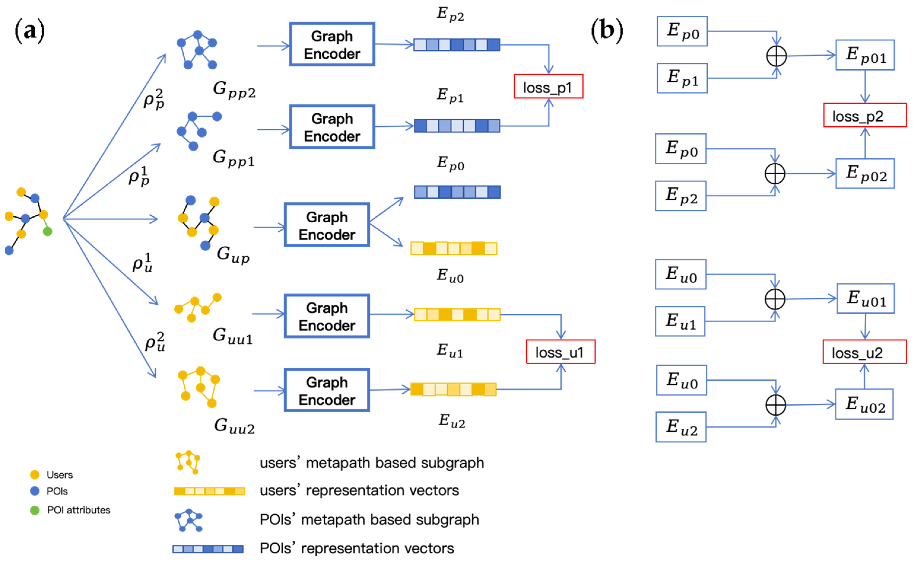
To address the aforementioned limitation (1), this paper employs a heterogeneous graph neural network to model the heterogeneous relations between users and POIs. When considering heterogeneous graphs, most studies only consider whether there is an interaction relation between users and POIs, often overlooking the potential high-order connections between them. Additionally, not all datasets contain sufficient information, particularly about users. The lack of user information can hinder the construction of a graph that accurately reflects user relations. To tackle these issues, we introduce a method using meta-paths as the solution. We firstly use the provided information in the datasets to construct a heterogeneous graph, including users, POIs, and POI attributes. As a valid tool for analyzing heterogeneous graphs, meta-paths can help identify potential connections between users and POIs. For instance, the meta-path UPU represents two users who have visited the same POI. By using different meta-paths, we can capture various types of connections between users and POIs, thereby constructing different meta-path-based subgraphs. To enhance the quality of the representation vectors, contrastive learning is applied to promote the representation learning of the heterogeneous graph and the meta-path subgraphs. Specifically, it designs two kinds of contrastive learning methods based on different meta-paths to learn the representation vectors of users and POIs.

To address the aforementioned limitation (2), we utilize graph structure learning to continuously refine the artificially constructed graph. The artificially constructed graph may contain noise and is not always complete. To tackle this problem, researchers have introduced graph structure learning, which aims to learn a more optimal graph structure though the training pipeline rather than directly using the original one without any modification. Most graph structure learning methods use a hybrid approach, where both the graph structure and GNN parameters are updated in conjunction with downstream tasks. In this study, the meta-path subgraphs used to learn the representations of users and POIs are artificially constructed graphs. Directly utilizing these graphs might result in inaccurate connections between nodes. Therefore, this paper employs graph structure learning to continuously optimize the structure of these meta-path subgraphs, thereby achieving more accurate relations between nodes.

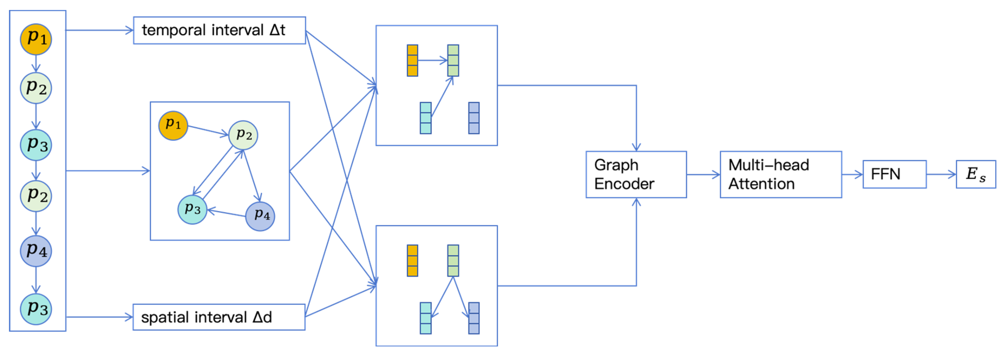
To address the aforementioned limitation (3), this paper employs graph neural networks to model users’ preferences in check-in sequences. To capture the connections between different check-ins, we first convert each check-in sequence into a sequence graph, and then use graph neural networks to learn these connections, treating the POIs visited by users as nodes and encoding the users’ sequence graphs using a graph encoder based on the attention mechanism. Given that users’ check-in behaviors are influenced by multiple factors, this paper incorporates time, space, and sequence into the computation of the graph convolutional neural network, thereby better generating the users’ preference representations.

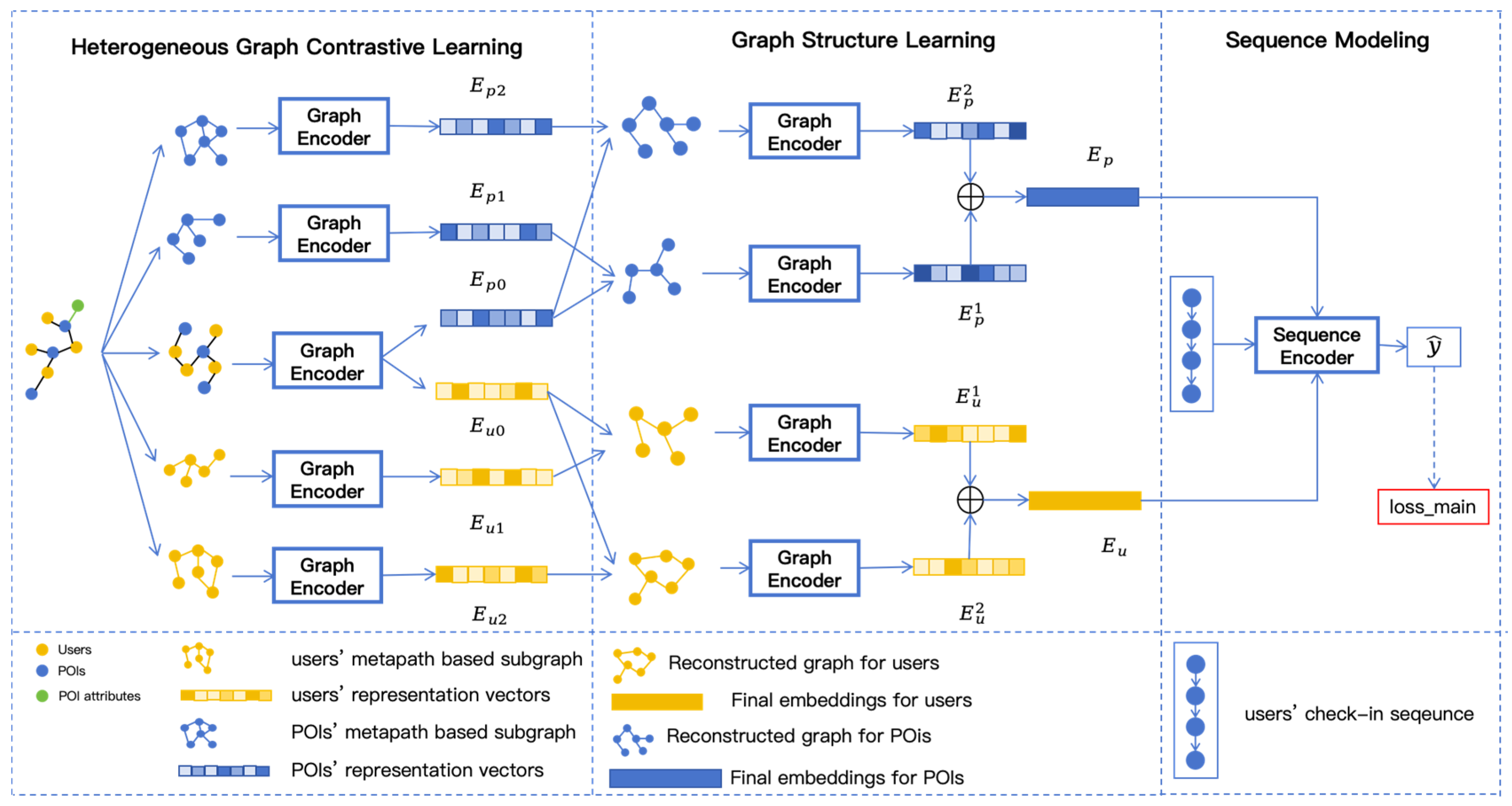
Based on the above analysis, we propose a model named Heterogeneous Graph Structure Learning for Next POI Recommendation (HGSL-POI). This model integrates heterogeneous graph contrastive learning, graph structure learning, and sequence modeling. Specifically, we consider the heterogeneous information between users, POIs, and POI attributes, and construct meta-path-based subgraphs for both users and POIs based on different meta-paths. Then, representation vectors for users and POIs are aligned through two contrastive learning methods, which differ in whether they consider the heterogeneous relation when computing the contrastive loss between different meta-path subgraphs. Next, the representation vectors obtained from contrastive learning are used to reconstruct the corresponding meta-path subgraphs, and graph neural networks are employed to obtain the representation vectors for users and POIs from the reconstructed graphs. Finally, the learned representation vectors for users and POIs are used to learn user sequences, where different types of factors will be included in this stage.

In summary, the main contributions of this paper are summarized as follows:

(1)

In this paper, heterogeneous graph contrastive learning is introduced into the process of representation learning. Considering the missing information may impact how we construct contrastive views, we use the provided information to construct a heterogeneous graph. Then, meta-paths are used to construct meta-path subgraphs of users and POIs, respectively, and two kinds of contrastive learning methods are adopted to improve the quality of the representation vectors of users and POIs.

(2)

Considering that the artificially constructed graph may have downsides such as noise and missing edges, graph structure learning is used to continuously update the graph structure, and takes the representation vectors generated by the updated graph as the input of the subsequent sequence modeling.

(3)

This paper models the users’ check-in sequences from the perspective of the graph, better capturing the relation between different check-ins. In addition to the sequential factor, we also include temporal and spatial factors into the modeling process to better capture the users’ preferences.

(4)

A large number of experiments are carried out on the public datasets, and the experimental results confirm the effectiveness of the model.

2. Literature Review

Based on the research content of this paper, the literature review is divided into three aspects: next point-of-interest recommendation, heterogeneous graph representation learning, and graph structure learning.

2.1. Next Point-of-Interest Recommendation

The next point-of-interest models are mainly divided into two categories: the first category is based on sequential models, and the second category is based on graph neural network models. Among the graph-based models, some papers choose to use self-supervised learning to assist the recommendation process.

Sequence-based models primarily view a user’s check-in history as a sequence, learning from this sequence to predict future check-ins. Early models often utilized Markov Chains (MCs) and Matrix Factorization (MF) techniques, such as FPMC [1], which combined MC and MF by decomposing the users’ transition matrix to capture long-term preferences. However, with the advancement of deep learning, many researchers have turned to Recurrent Neural Networks (RNNs) and their variants, which offer significant advantages in sequential modeling. For example, ST-RNN [6] integrates spatiotemporal context into the RNN-based neural network layer. In LSPL [19] and PLSPL [20], LSTM is used to capture short-term preferences. STGN [21] employs two time gates and two distance gates to capture spatiotemporal features in both long-term and short-term preferences. STAN [22] uses an attention mechanism to capture relations between non-adjacent check-ins, while also incorporating spatiotemporal information.

Sequence-based models can only focus on the users’ local context and cannot capture their behaviors from a global perspective. In contrast, graph neural networks can model the connections between users and POIs from a broader perspective. For example, GE [10] has constructed several relation graphs between users and POIs, resulting in representation vectors for both users and POIs. HMT-GRN [23] has created a user-region matrix to reduce the sparsity of the interaction matrix between users and POIs. GETNext [15] believes that recommending the next point-of-interest is not just a sequential recommendation task. In addition to use Transformer-based sequential modeling, it also constructs a trajectory graph reflecting the order of users’ check-ins. This graph helps learn the probability of users moving from the current POI to any other POIs, which is then added to the sequence recommendation results. The STHGCN [16] model uses hypergraphs to capture high-order information, linking user history trajectories with the check-in patterns of different users.

Self-supervised learning has emerged as a promising method in deep learning. In next POI recommendation, this method can help capture users’ latent preferences or the potential relations between POIs, improving the performance of personalized recommendation. For example, GSBPL [24] considers the sequential visits in the graph and uses two augmentation strategies, edged masking and bridging, as well as edge inversion, to create different views for graph contrastive learning. SLS-REC [25] uses a node drop strategy to generate views for the contrastive learning of users’ long-term and short-term interests. LSPSL [26] focuses on data sparsity and dynamic user preference. The authors design two objectives to enhance sequence representations by exploiting the spatio-temporal context. CLLP [27] considers users’ preference diversity and data sparsity and propose to remove noise from POI representations by leveraging the collaborative signals from other users. These papers have validated the self-supervised-learning-based method in POI recommendation.

2.2. Heterogeneous Graph Representation Learning

Heterogeneous graphs, which include more than one kind of nodes and edges, are more prevalent in real-world scenarios and can contain more kinds of relations within the graph. The goal of representation learning in heterogeneous graphs is to obtain node representation vectors while preserving the graph heterogeneity. To achieve high-quality node representation vectors in heterogeneous graphs, several studies have proposed methods for node-embedding learning. For example, HAN [28] uses meta-paths and hierarchical attention mechanisms to capture relations at both the node and meta-path levels, from the perspectives of nodes and semantic information. HGT [29] integrates the Transformer architecture with graph theory, designing different information aggregation methods for nodes based on their relations. MAGNN [30] aggregates node information through various meta-paths.

The core concept of contrastive learning is to achieve better representation vectors by bringing positive samples closer together and negative samples farther apart. Some studies have applied contrastive learning to heterogeneous graph neural networks, thereby enhancing downstream tasks. For example, HeCo [31] leverages the network structure and meta-paths of graphs to construct different views and uses contrastive learning to align positive samples; HGCML [32] constructs different views solely through meta-paths; HGMAE [33] enhances model performance by using meta-paths, node attribute-level masking mechanisms, and position predictions; and IHGCL [34] generates different node views through various meta-paths and improves the quality of node representation vectors using different methods of contrastive learning. MEOW [35] is proposed to address the limitations of the neglecting of meta-path contexts and the inability to distinguish between hard and false negative samples. Two views are proposed to aggregate and encode meta-paths and a weighted contrastive loss to differentiate negative samples. As data sparsity and domain differences exist in cross-domain recommendation, HGCCDR [36] constructs heterogeneous graphs, and leverages intra- and inter-domain augmentation strategies and contrastive learning to align domain-independent features. HGCL [37], a robust self-supervised framework for heterogeneous graphs, uses a reciprocal contrastive mechanism to address noise in node attributes and topology by introduce two corresponding reviews. MTDG [38] leverages four encoders to capture knowledge in local, global, long-term, and short-term situations, respectively. The authors also propose single-contrastive and cross-contrastive learning to optimize the learned embeddings. M2CHGNN [39] leverages a two-level attention mechanism with contrastive learning. Meta-paths and meta-structures are used to capture complex relations within heterogeneous graphs and a contrastive learning framework aligns these views.

2.3. Graph Structure Learning

Although graph neural networks have achieved significant success in addressing graph-related problems, many models still use artificially defined graphs that may contain noise or missing edges. This can degrade the quality of the representation vectors and, in the end, affect the performance of downstream tasks. To address the uncertainties in graphs, some models are proposed to use graph structure learning to learn an optimal graph structure during training process. Graph structure learning research can be broadly categorized into three types: metric learning, probabilistic modeling, and direct optimization.

Models based on metric learning calculate the similarity between nodes by their representation vectors, thereby updating the probability of edges existing between nodes. For example, IDGL [40] alternates between learning the graph structure and the representation vectors, assuming that a good graph structure can generate a good representation vector, and vice versa. AGCN [41] learns a task-oriented adaptive graph structure for each graph dataset during training, using distance metric learning to learn the graph structure. AM-GCN [42] extracts embeddings from node features, the graph’s topological structure, and their combinations, and uses an attention mechanism to learn weights.

The model based on probabilistic modeling learns a probability distribution related to the edges from the graph, and then samples a graph from this distribution. For example, LDS [43] learns the discrete probability distribution of the graphs edges by solving a two-layer program that combines the graph structure and GCN parameters, and then samples the graph structure from this distribution. PTDNet [44] enhances the robustness and generalization of GNNs by discarding edges irrelevant to the task. NeuralSparse [45] uses both structural and non-structural information as inputs, employing neural networks to sparsify the graph structure and remove edges that may be irrelevant to the task.

The direct optimization model treats the adjacency matrix of the graph as parameters, optimizing it alongside other GNN parameters. For example, GLNN [46] optimizes the graph directly using data and tasks. ProGNN [47] leverages the unique properties of the graph to optimize both its structure and GNN parameters, aiming to simultaneously learn better graph structures and GNN models from the perturbed graph. TO-GCN [48] uses labels to optimize the parameters of the adjacency matrix and to learn the GNN parameters. GCEN [49] addresses the challenges of missing or misconnected graph structures in the real world and employ a multi-branch generation structure to obtain diverse graph topologies. BiGSL [50] considers the hierarchical relations among POIs and the graphs often suffer from noise or incompleteness. A hierarchical graph is iteratively learned to refine the graph structures. Additionally, it employs a contrastive multiview fusion to increase the recommendation performance. RGSL [51] considers the challenge in heterophilic graphs, where connected nodes may have different labels. It uses a filter to enhance node distinctiveness and a contrastive regularizer to refine the graph’s structure.

3. Problem Definition

We use $U=\{u_1,u_2,\dots ,u_M\}$ to represent the user set, $P=\{p_1,p_2,\dots ,p_N\}$ to represent the POI set, and $C=\{c_1,c_2,\dots ,c_K\}$ to represent the attributes which the POIs have, where M, N, and K are the total number of users, POIs, and attributes, respectively. Each POI p is denoted by a quadruple p = (id, lon, lat, attr), which includes the id, longitude, latitude, and attributes of the POI.

Check-in. A check-in is represented by a triplet q = (u, p, t), which represents that user u visited POI p at time t.

Sequence and check-in history. A sequence is a set of continuous check-ins of a user within a period of time. We use $s_m^u=\{q_1^u,q_2^u,\dots q_n^u\}$ to represent the m-th sequence of user u, which includes n check-ins. $q_k^u=(u,p_k^u,t_k^u)$ denotes the k-th check-in of the sequence, where k is a positive integer. Considering two sequences $s_n^v$ and $s_m^u$, if $s_n^v$ ends before $s_m^u$ starts, we denote $s_n^v$ as the historical sequences of $s_m^u$. The historical sequences of a user includes the sequences belonging to the same user and different users. All the check-in sequences of the same user constitute the check-in history of the user, which is denoted by $S^u=\{s_1^u,s_2^u,\dots s_{\left|S^u\right|}^u\}$, where ${|S}^u|$ is the number of check-in sequences of user u.

The next point-of-interest recommendation aims to provide a list of POIs which a user is most likely to visit in the future, based on the current sequence and the historical sequences of all users. This list ranks the POIs in order of the probabilities. Specifically, given the set of all users’ historical check-in sequences ${\left\{S^u\right\}}_{u\in U}$ and the current sequence $s^{u_i}=\{q_1^{u_i},q_2^{u_i},\dots q_n^{u_i}\}$ of user $u_i$, the next point-of-interest recommendation is to predict where the users will visit at the future time $t_{\mathrm{n}+1}$:

$${\widehat{y}}_i=f\left(p_i\right|{S^1,S^2,\dots ,S^M,s}^{u_i},t_{n+1})$$

where ${\widehat{y}}_i$ represents the probability of the user visiting POI $p_i$, f represents the model parameters, and $S^1,S^2,\dots ,S^M$ represents the historical sequences of the user, including the sequences of the same user and different users.

4. Heterogeneous Graph Structure Learning Model

4.1. Model Structure Overview

The proposed heterogeneous graph contrastive learning model for next POI recommendation (HGSL-POI) is illustrated in Figure 1. The model comprises three main components: (1) the heterogeneous graph contrastive learning; (2) the graph structure learning; (3) the sequence modeling. Specifically, in the heterogeneous graph contrastive learning component, we first construct a heterogeneous graph at the leftmost part in Figure 1. Then, we extract the interaction graph and four meta-path-based subgraphs according to different meta-paths from the constructed heterogeneous graph. Different graph encoders are used to learn the representation vectors for different graphs. Note the graph encoder in the middle produce representations for users and POIs since it operates on the user-POI interaction graph, while other encoders only yield representations for one type of node. Then, we use two types of contrastive learning methods to assist the learning of representation vectors for users and POIs. How the contrastive learning works is provided in Figure 2, Section 4.2. After we obtain the representations from different encoders, we use graph structure learning to reconstruct the corresponding meta-path-based subgraphs. By feeding the reconstructed graphs into graph encoders, we can obtain the final representations for users and POIs. The graph structure learning process can be found in Section 4.3. Finally, the sequence modeling uses the representations from graph structure learning and the users’ check-in sequences, supplemented by other extra information such as time and distance, to predict the POIs that users are likely to visit in the future. Due to the space constraints, we put the details of sequence modeling in Section 4.4.

4.2. Heterogeneous Graph Contrastive Learning

This section primarily discusses the heterogeneous graph contrastive learning, which is the first part of our proposed model. In our model, we use two kinds of contrastive learning methods to help generate representations of users and POIs. The details can be found in Figure 2a,b. Figure 2a includes the process of generating subgraphs based on the meta-paths, encoding these meta-path-based subgraphs and the first kind of contrastive learning method, which we call meta-path-based graph contrastive learning in this paper. First, we construct a graph including users, POIs, and POI attributes. Since there is more than one type of node, the constructed graph is definitely a heterogeneous graph. For users, we use two meta-paths ${\rho }_u^1$ and ${\rho }_u^2$ to construct users’ meta-path-based subgraph $G_{uu1}$ and $G_{uu2}$, while, for POIs, we obtain $G_{pp1}$ and $G_{pp1}$ based on ${\rho }_p^1$ and ${\rho }_p^2$. To model the interaction relation between users and POIs, we also extract the interaction graph $G_{up}$. Then, we use different graph encoders to encode these graphs and obtain the representations for different nodes. Finally, we use the meta-path-based contrastive learning to learn representations for users and POIs. This contrastive learning works between different meta-paths of the same node type. Figure 2b illustrates another kind of contrastive learning method, which we call interaction-aware contrastive learning. This contrastive learning considers the representations from the interaction graph. We first fuse the representations of the same node type from the interaction graph with others from the meta-path-based subgraphs. Then, we calculate the contrastive loss in a similar way. We divide the heterogeneous graph contrastive learning component into three subsections: the construction of meta-path-based subgraphs, heterogeneous graph representation learning, and heterogeneous graph contrastive learning. More details can be found in the following subsections.

4.2.1. Construction of Meta-Path-Based Subgraphs

To obtain a more comprehensive node relation, this paper first constructs a heterogeneous graph G = (V, E), where the nodes include users, POIs, and POI attributes which the POIs have. Edges are constructed according to the following rules: if user u has visited a POI p, then the user is connected to the POI; if a POI has a specific attribute, then the POI is connected to this attribute. Note that all edges in G are undirected.

Based on the heterogeneous graph G, this paper first extracts the interaction graph $G_{up}$ between users and POIs. $G_{up}$ includes all users and POIs. If user u has visited POI p, there is an edge between u and p. The adjacency matrix of $G_{up}$ is $A_{up}$.

In addition to the interaction graph, we also construct different subgraphs for users and POIs based on different meta-paths in order to capture the potential high-order connections between nodes. The meta-path is widely used in heterogeneous graphs to illustrate how two nodes connect. For example, the meta-path UPU indicates that two users are connected through a POI, which means they have visited the same POI. Maybe these two users have similar interests. The meta-path PCP indicates that two POIs belong to the same category. A user may choose another POI for substitution.

The meta-path subgraphs are constructed based on the following rules: for a given node v with node type $v_1$ and a meta-path $\rho$, we can find all the other nodes connected to node v through the meta-path $\rho$. Then, we treat these selected nodes to be connect with node v and denote this connection as $e_{\rho }^v$. By applying the above process to all the nodes of type $v_1$, we can obtain all the connections $E=\left\{e_{\rho }^v\right|v\in V_1\}$. Then, we can construct meta-path subgraph $G_{v1}^{\rho }$ utilizing the nodes of node type $v_1$ and the connections E between them. For example, if two users are connected by UPU, they are connected in the meta-path subgraph; otherwise, they are not connected. By applying this procedure to all users, we can obtain the meta-path graph $G_U^{UPU}$ for the user and UPU. This method has nothing to do with whether there is a direction between these two nodes or not.

According to the definition of the meta-path and meta-path-based subgraph, we select two meta-path-based subgraphs $G_{uu1}$ and $G_{uu2}$ for users based on meta-paths ${\rho }_u^1$ and ${\rho }_u^2$ and two meta-path-based subgraphs $G_{pp1}$ and $G_{pp2}$ for POIs based on meta-paths ${\rho }_p^1$ and ${\rho }_p^2$. The adjacency matrix of each meta-path-based subgraph is $A_{uu1}$, $A_{uu2}$, $A_{pp1}$, and $A_{pp2}$, respectively. These subgraphs illustrate the potential high-order relations between nodes of the same type, which can be useful even when lacking relevant information. For example, if the users’ friend list is unavailable, it is impossible to determine the connections between users. However, subgraphs based on meta-paths can help identify these connections to some extent. Different meta-paths can carry distinct semantic information, and, by constructing different meta-paths and subgraphs, we can gain a more comprehensive understanding of the relations between nodes. These four meta-path subgraphs and $G_{up}$ constitute the input of heterogeneous graph representation learning.

4.2.2. Heterogeneous Graph Representation Learning

In the previous section, we constructed different subgraphs based on various meta-paths. To better model the higher-order relations in the graph, this paper employs graph neural networks to encode these subgraphs. Before using neural networks for encoding, we first generated a representation vector for each user and POI based on their ID, denoted as ${\mathrm{e}}_{\mathrm{u}}\in {\mathrm{R}}^d,{\mathrm{e}}_{\mathrm{p}}\in {\mathrm{R}}^d$, where d represents the embedding dimension of the vector. Based on ${\mathrm{e}}_u$ and ${\mathrm{e}}_p$, the initial embedding matrices for all users and POIs are ${\mathrm{E}}_u^0\in {\mathrm{R}}^{M\times d},{\mathrm{E}}_p^0\in {\mathrm{R}}^{N\times d}$, respectively, where M and N represent the number of users and POIs. To better distinguish different types of entities, this paper employs a self-gating mechanism [52] to further initialize the representation vectors of the input meta-path subgraphs, as follows:

$${\mathrm{E}}_{uu}^0={\mathrm{E}}_u^0⨀\mathsf{\sigma }({\mathrm{E}}_u^0{\mathrm{W}}_u+{\mathrm{b}}_u);{\mathrm{E}}_{pp}^0={\mathrm{E}}_p^0⨀\mathsf{\sigma }({\mathrm{E}}_p^0{\mathrm{W}}_p+{\mathrm{b}}_p)$$

(1)

where ${\mathrm{E}}_{uu}^0\in {\mathrm{R}}^{M\times d}$ is the input of ${\mathrm{G}}_{uu1}$ and ${\mathrm{G}}_{uu1}$, ${\mathrm{E}}_{pp}^0\in {\mathrm{R}}^{N\times \mathrm{d}}$ is the input of ${\mathrm{G}}_{pp1}$ and ${\mathrm{G}}_{pp2}$, $\mathsf{\sigma }$ is the sigmoid nonlinear activation function, ${\mathrm{W}}_u$, ${\mathrm{W}}_p$, ${\mathrm{b}}_u$, and ${\mathrm{b}}_p$ are learnable parameters, and ⊙ denotes element-wise multiplication. We can obtain ${\mathrm{E}}_{uu}^0$ and ${\mathrm{E}}_{pp}^0$ by (1), which will be used as the input to the meta-path subgraph encoders, while the input of ${\mathrm{G}}_{up}$ is the initial representation ${\mathrm{E}}_u^0$ and ${\mathrm{E}}_p^0$.

After obtaining the initial representation vectors, a graph neural network is used to further extract higher-order features for meta-path subgraphs ${\mathrm{G}}_{uu1}$, ${\mathrm{G}}_{uu2}$, ${\mathrm{G}}_{pp1}$, and ${\mathrm{G}}_{pp2}$. We use different graph encoders for representation learning:

$$\begin{gathered} E_{u1}^l=\mathrm{G}\mathrm{N}\mathrm{N}(A_{uu1},E_{u1}^{l-1}),E_{u2}^l=\mathrm{G}\mathrm{N}\mathrm{N}(A_{uu2},E_{u2}^{l-1}) \\ {E}_{p1}^l=\mathrm{G}\mathrm{N}\mathrm{N}(A_{pp1},E_{p2}^{l-1}),E_{p2}^l=\mathrm{G}\mathrm{N}\mathrm{N}(A_{pp1},E_{p2}^{l-1}) \end{gathered}$$

(2)

Among them, GNN represents the encoder based on a graph neural network. In our work, GIN [53] is used as the encoder to process meta-path subgraph representation learning. ${\mathrm{E}}_{u1}^l$, ${\mathrm{E}}_{u2}^l$, ${\mathrm{E}}_{p1}^l$, and ${\mathrm{E}}_{p2}^l$ are the node representations after the aggregation of the graph neural network at the l-th layer, and the initialization representations at the 0-th layer are ${\mathrm{E}}_{u1}^0$, ${\mathrm{E}}_{u2}^0$, ${\mathrm{E}}_{p1}^0$, and ${\mathrm{E}}_{p2}^0$ from (1). After l iterations, we take the output of the last layer as the final result, where l is the number of layers of the graph encoders. The final output ${\mathrm{E}}_{u1}$, ${\mathrm{E}}_{u2}$, ${\mathrm{E}}_{p1}$, and ${\mathrm{E}}_{p2}$ are used as the input for subsequent contrastive learning and graph structure learning.

For $G_{up}$, we use LightGCN [54] to obtain the representation vectors:

$${\mathrm{E}}_{u0},{\mathrm{E}}_{p0}=\mathrm{L}\mathrm{i}\mathrm{g}\mathrm{h}\mathrm{t}\mathrm{G}\mathrm{C}\mathrm{N}(A_{up},{\mathrm{E}}_u^0|\left|{\mathrm{E}}_p^0\right)$$

(3)

Specifically, we have the following:

$$e_u^l=\sum _{p\in N_u}{\displaystyle \frac{1}{\sqrt{\left|N_u\right|\left|N_p\right|}}}{e}_p^{l-1},e_p^l=\sum _{u\in N_p}{\displaystyle \frac{1}{\sqrt{\left|N_p\right|\left|N_u\right|}}}{e}_u^{l-1}$$

(4)

where $N_u$ and $N_p$ denote the first-order neighbors of user u and POI p. ${\mathrm{e}}_u^l$ and ${\mathrm{e}}_p^l$ are the representations of users and POIs after the l-th layer of aggregation, while the initialization representation of the 0-th layer is ${\mathrm{E}}_u^0$ and ${\mathrm{E}}_p^0$, respectively. Compared to the traditional graph convolution neural network (GCN), LightGCN eliminates the linear transformation and learnable parameters, thereby improving the model efficiency. Similarly, after l iterations, we use the output of the final layer as the final result, denoted as ${\mathrm{E}}_{u0}$ and ${\mathrm{E}}_{p0}$, which will be used as the input of subsequent heterogeneous graph contrastive learning.

4.2.3. Heterogeneous Graph Contrastive Learning

To further enhance the quality of the representation vectors obtained by the graph encoders, this paper employs graph contrastive learning to align the representation vectors from different subgraphs. The goal of graph representation learning is to align the node representation vectors, with the core idea being that similar samples are brought closer together, while dissimilar samples are pushed further apart. To incorporate information from various aspects, this paper adopts two methods of contrastive learning:

(1)

Meta-path-based Contrastive Learning

The meta-path-based contrastive learning is mainly to align the representation vectors of users and POIs under meta-path subgraphs. The representation vectors used in this part are ${\mathrm{E}}_{u1},{\mathrm{E}}_{u2},{\mathrm{E}}_{p1}\mathrm{a}\mathrm{n}\mathrm{d}{\mathrm{E}}_{p2}.$ $\mathrm{T}\mathrm{a}\mathrm{k}\mathrm{e}$ the loss function of users as an example. We use the representations ${\mathrm{E}}_{u1}$ and ${\mathrm{E}}_{u2}$ from different meta-paths and the InfoNCE loss function to align the two representations and maximize the mutual information between them. The specific calculation method is as follows:

$$L_{u1}=\sum _{u\in U}-log{\displaystyle \frac{exp\left(sim\right(e_u^1,e_u^2)/\tau )}{\sum _{u^{\prime }\in U}exp\left(sim\right(e_u^1,e_{u^{\prime }}^2)/\tau )}}$$

(5)

where ${\mathrm{e}}_u^1$ and ${\mathrm{e}}_u^2$ are the representations of the same user u under two meta-path subgraphs, ${\mathrm{e}}_{u‘}^1$ is the representation for another user u′, sim is the cosine similarity, and $\tau$ represents the temperature coefficient, which can be used to control the model’s ability to distinguish between different negative samples. In this paper, the representations of the same user under different subgraphs are considered positive samples and should be as similar as possible. Conversely, the representations of different users are considered negative samples and should be as dissimilar as possible. The goal of the contrastive learning in the meta-path subgraphs is to align the node representations under different relations. Based on this method, we can obtain the $L_{p1}$ for ${\mathrm{E}}_{p1}\mathrm{a}\mathrm{n}\mathrm{d}{\mathrm{E}}_{p2}$:

$$L_{p1}=\sum _{p\in U}-log{\displaystyle \frac{exp\left(sim\right({\mathrm{e}}_p^1,e_p^2)/\tau )}{\sum _{p^{\prime }\in P}exp\left(sim\right({\mathrm{e}}_p^1,{\mathrm{e}}_{p^{\prime }}^2)/\tau )}}$$

(6)

(2)

Interaction-Aware Contrastive Learning

Based on four meta-path subgraphs and the interaction graph, the interaction-aware contrastive learning takes into account the interaction graph between users and POIs. Take the calculation of user contrastive loss as an example. Before calculating the contrastive loss, we first integrate the representation vectors from the meta-path subgraphs with those from the heterogeneous interaction graph to obtain the user representation vectors. The integration method is as follows:

$${\mathrm{E}}_{u01}={\mathrm{E}}_{u1}⨁{\mathrm{E}}_{u0},{\mathrm{E}}_{u02}={\mathrm{E}}_{u2}⨁{\mathrm{E}}_{u0}$$

(7)

where ${\mathrm{E}}_{u1}$ and ${\mathrm{E}}_{u2}$ are the results of the meta-path subgraph coding, ${\mathrm{E}}_{u0}$ is the representations of users obtained from the interaction graph, $⨁$ is average pooling, ${\mathrm{E}}_{u01}$ and ${\mathrm{E}}_{u02}$ are the results of the fusion between the representations of meta-path subgraphs and the representations obtained from the heterogeneous graph. In order to learn the information of the meta-path subgraph enhanced by heterogeneous information, we use the following method to calculate the contrast loss:

$$L_{u2}=\sum _{u\in U}-log{\displaystyle \frac{exp\left(sim\right(e_u^{01},e_u^{02})/\tau )}{\sum _{u^{\prime }\in U}exp\left(sim\right(e_u^{01},e_{u^{\prime }}^{02})/\tau )}}$$

(8)

where ${\mathrm{e}}_u^{01}$ and ${\mathrm{e}}_u^{02}$ are the same user u’s representations in ${\mathrm{E}}_{u1}$ and ${\mathrm{E}}_{u2}$, ${\mathrm{e}}_{u^{\prime }}^{02}$ is the representation for another user u′, and $\tau$ is the temperature coefficient. In a similar way, we can obtain the $L_{p2}$ for ${\mathrm{E}}_{p0}$, ${\mathrm{E}}_{p1}\mathrm{a}\mathrm{n}\mathrm{d}{\mathrm{E}}_{p2}$

$$E_{p01}=E_{p1}⨁E_{p0},E_{p02}=E_{p2}⨁E_{p0}$$

(9)

$$L_{p2}=\sum _{p^{\prime }\in P}-log{\displaystyle \frac{exp\left(sim\right(e_p^{01},e_p^{02})/\tau )}{\sum _{p^{\prime }\in P}exp\left(sim\right(e_p^{01},e_{p^{\prime }}^{02})/\tau )}}$$

(10)

(3)

The complementary roles of the two contrastive learning methods

In our proposed model, we proposed the use of two kinds of contrastive learning methods to help generate representations for users and POIs. The first kind of method merely considers the meta-path-based subgraphs, while the second one includes the interaction relation between users and POIs. In this subsection, the difference between them and the necessities to use them, especially the second one, are illustrated.

First, we argue they can capture the relations from complementary perspectives. The meta-path-based graph contrastive learning method only considers the homogeneous relations, since the meta-path-based subgraphs only capture the relations within the same type of node, whether for the users or POIs, while the second one, interaction-aware contrastive learning, includes high-order heterogeneous relations between users and POIs. As a result, the interaction-aware contrastive learning captures the interaction relation between users and POIs, while the meta-path-based graph contrastive learning captures the relation between users or POIs. They capture the relations from different perspectives, and can complement each other.

As we use the Graph Neural Network (GNN) to perform graph representation learning on the constructed graphs, the interaction graph allows us to model the relations among users and POIs, which cannot be captured by meta-path-based subgraphs. By performing the GNN on the interaction graph, we can obtain the representation vectors of users and POIs, considering the interaction relations between them.

4.3. Graph Structure Learning

Although subgraphs constructed based on meta-paths can capture the relations between nodes from various perspectives, the noise and missing key edges in the graph may affect the encoding results, which, in the end, may impact the final recommendation outcomes. Such manually defined graphs often contain redundant edges and miss some critical ones. Graph structure learning continuously optimizes the graph structure during training, thereby obtaining higher-quality representation vectors based on the continuously optimized graph.

In this part, we use graph structure learning to continuously update the meta-path subgraph. This part use ${\mathrm{E}}_{u0}$, ${\mathrm{E}}_{u1}$, ${\mathrm{E}}_{u2},$ ${\mathrm{E}}_{p0}$, ${\mathrm{E}}_{p1}$, $\mathrm{a}\mathrm{n}\mathrm{d}$ ${\mathrm{E}}_{p2}$ as the input. When reconstructing a subgraph of a meta-path, the representations obtained from the subgraph and the corresponding node representation from the interaction graph are used. For example, when reconstructing $G_{uu1}$, we use ${\mathrm{E}}_{u1}$ obtained from $G_{uu1}$ and the user representations from ${\mathrm{E}}_{u0}$. The process can be expressed as follows:

$$E_{i,j}^{uu1}=\sum _{g\in \{G_{uu1},G_{up\}}}{\beta }_g(cos(e_i^g,e_j^g))$$

(11)

where $E_{i,j}^{uu1}$ indicates the probability whether there is an edge between node i and j, g represents the graph, which includes $\{G_{uu1},G_{up}\}$, ${\beta }_g$ is a hyper-parameter used to balance the importance of different graphs, cos is the cosine similarity calculation function, and ${\mathrm{e}}_i^g$ and ${\mathrm{e}}_j^g$ are the representations of node i and j in the graph g. Then, we remove $m^{-}$ edges with the lowest probabilities and add the the most probable $m^{+}$ edges. By doing so, we can obtain the optimized graph $G_{u1}$. In a similar way, we can obtain $G_{u2}$ using ${\mathrm{E}}_{u2}$ and ${\mathrm{E}}_{u0}$, $G_{p1}$ using ${\mathrm{E}}_{p1}$ and ${\mathrm{E}}_{p0}$, and $G_{p2}$ using ${\mathrm{E}}_{p2}$ and ${\mathrm{E}}_{p0}$. We use the heuristic method to reduce the memory overload by avoiding back-propagation through dynamic graph operations. Moreover, the heuristic method increases the interpretability when we add or remove edges. The cosine-similarity threshold provides explicit control over edge sparsity and semantic consistency, while, if we use differentiable graph learning, the learned edge weights lack the explainability.

After obtaining the four optimized graphs, we can obtain the representation vectors of nodes by using different graph neural networks for encoding. The calculation method is as follows:

$$\begin{gathered} {\mathrm{E}}_u^1=\mathrm{G}\mathrm{N}\mathrm{N}(A_{u1},{\mathrm{E}}_{u1}^l),{\mathrm{E}}_u^2=\mathrm{G}\mathrm{N}\mathrm{N}(A_{u2},{\mathrm{E}}_{u2}^l) \\ {\mathrm{E}}_p^1=\mathrm{G}\mathrm{N}\mathrm{N}(A_{p1},{\mathrm{E}}_{p2}^l),{\mathrm{E}}_p^2=\mathrm{G}\mathrm{N}\mathrm{N}(A_{p1},{\mathrm{E}}_{p2}^l) \end{gathered}$$

(12)

where $A_{u1}$, $A_{u2}$, $A_{p1}$, and $A_{p2}$ are the adjacency matrices of $G_{u1}$, $G_{u2}$, $G_{p1}$, and $G_{p2}$, and ${\mathrm{E}}_u^1$, ${\mathrm{E}}_u^2$, ${\mathrm{E}}_p^1$, and ${\mathrm{E}}_p^2$ are the results of graph encoding. Then, the representation vectors of users and POIs are fused, respectively, to obtain the final representations:

$${\mathrm{E}}_{\mathrm{u}}={\mathrm{E}}_u^1⨁{\mathrm{E}}_u^2,{\mathrm{E}}_p={\mathrm{E}}_p^1⨁{\mathrm{E}}_p^2$$

(13)

where $⨁$ denotes the average pooling, and ${\mathrm{E}}_u$ and ${\mathrm{E}}_p$ are the final representations of users and POIs, which will then be applied in the sequence modeling.

4.4. Sequence Modeling

The check-in sequence of users reflects the correlation between POIs in the order of visits. The sequence modeling is the ultimate component of our proposed model. By learning the users’ sequence preferences, we can predict where the users may visit in the future. In order to accurately capture users’ sequence preferences, we divide this component into two parts: the construction of sequence graphs and sequence encoding. Specifically, we first transform each sequence into a graph based on the order of the visited POI within the sequence. At the same time, we extract the temporal interval and geographical distance between consecutive check-ins. Moreover, considering that using the entire check-in history may add too much noise and the only current sequence may not provide enough information, we use the Jaccard index to help choose similar sequences. After we obtain the sequence graphs, we design a GNN-based graph encoder to encode these graphs. This graph encoder takes sequence graphs, temporal intervals, and geographical distances as the input, and generates the representations for these graphs. These representations can also reflect users’ sequence preferences. More details can be found in the following subsections.

4.4.1. Construction of Sequence Graphs

For any given sequence s, we transform the sequence into a graph $G_s$, which captures the correlation between nodes from the graph perspective. Specifically, the graph $G_s$ uses the visited POIs as nodes and the order of user visits as edges. In other words, if a user visits POI i and then POI j in the same sequence, there is a directed edge from node i to j. Additionally, to capture the spatio-temporal relation between two check-ins, we also consider the time interval and spatial interval between two check-ins.

Unlike the sequential model, which can only learn about the information related to visited points, using a graph data structure can better capture the connections between different POIs, especially those between non-adjacent POIs. However, considering only the current users’ trajectory may not fully reflect their behavior, as the same trajectory segments can lead to users visiting different POIs. Utilizing all the check-in history may also include much noise. Therefore, to better model sequence information, this paper extracts sequences from both the users’ historical sequences and that of other users, which can help predict where the user is inclined to visit. Specifically, for the currently known trajectory $s_1$, if there is a historical sequence $s_2$, which makes $Jaccard(s_1,s_2)$ large, we treat $s_2$ as a similar sequence to $s_1$. The Jaccard index is computed as follows (Reviewer 1, Comments 3):

$$\mathrm{J}\mathrm{a}\mathrm{c}\mathrm{c}\mathrm{a}\mathrm{r}\mathrm{d}({\mathrm{s}}_1,{\mathrm{s}}_2)={\displaystyle \frac{|s_1\cap s_2|}{|s_1\cup s_2|}}$$

(14)

Note that this paper distinguishes between whether a trajectory belongs to the same user when considering similar trajectories. We select $k_1$ sequences of the same user, and $k_2$ for different users. In the end, together with the current sequence, the total (${\mathrm{k}}_1$ + ${\mathrm{k}}_2$ + 1) sequences are used to construct the sequence graph.

The order of users’ visits is a critical factor when we are tackling the next POI recommendation task. The Jacarrd index is used to choose the similar sequences, while the order is considered in the construction of sequence graphs and the following sequence modeling. We separately considering choosing the similar sequences and the order of visits, allowing us to apply more complex order-based sequence preference learning.

4.4.2. Sequence Encoding

After constructing the user’s check-in sequence graph, this paper designs a graph encoder based on the attention mechanism to capture relations between POIs. Specifically, it extracts features of POIs from a graph perspective and aggregates them into a representation vector for the check-in sequence (see Figure 3 for the detailed architecture). In addition to the sequential order of visited POIs, the temporal and spatial information between two check-ins is equally critical. The impacts of time intervals and geographical distances vary: shorter time intervals reflect stronger correlations between POIs, and larger geographical distances may indicate shifts in user preferences. Thus, we integrate both temporal and spatial information into the sequence modeling process.

Specifically, for a trajectory graph $G_s$, the sequence representation is generated based on POI embedding $E_p$, time interval $\Delta t_{ij}$ and spatial distance $\Delta d_{ij}$ between two consecutive check-ins i and j, and the graph attention network (GAT). The attention coefficients are computed as follows:

$$a_{ij}=W\left({\mathrm{x}}_i^s\odot {\mathrm{x}}_j^s+\Delta d_{ij}+\Delta t_{ij}\right)$$

(15)

where $a_{ij}$ is the attention coefficient between nodes $i$ and $j$, ${\mathrm{x}}_i^s$ and ${\mathrm{x}}_j^s$ are POI representations from ${\mathrm{E}}_p$, and $\odot$ denotes element-wise multiplication. In addition, we argue the visited POI would not only be influenced by the previous visits, but also have a relation with the future one. Therefore, in order to model the bidirectional relations, we compute attention coefficients in two directions to model both historical and future influences:

$$\begin{gathered} a_{ij}^{\left(in\right)}=W^{\left(in\right)}\left({\mathrm{x}}_i^s\odot {\mathrm{x}}_j^s+\Delta d_{ij}+\Delta t_{ij}\right) \\ {a}_{ij}^{\left(out\right)}=W^{\left(out\right)}\left({\mathrm{x}}_i^s\odot {\mathrm{x}}_j^s+\Delta d_{ij}+\Delta t_{ij}\right) \\ {a}_{ij}=a_{ij}^{\left(in\right)}\parallel a_{ij}^{\left(out\right)} \\ {\mathrm{x}}_i^s=\sum _{j\in N_i}{a}_{ij}{\mathrm{x}}_j^s \end{gathered}$$

(16)

where $\parallel$ denotes a concatenation operation, $N_i$ is the set of neighboring nodes of i, and $x_i^s$ is the updated representation for POI i in the sequence. The final output can be represented as ${\mathrm{X}}^s=[{\mathrm{x}}_1^s,{\mathrm{x}}_2^s,\dots ,{\mathrm{x}}_{\mathrm{n}}^s]$. To further capture user preferences from multiple perspectives, we apply a self-attention mechanism to encode the node representation:

$${\mathrm{X}}_{seq}=\mathrm{F}\mathrm{F}\mathrm{N}\left(\mathrm{Attention}({\mathrm{W}}_Q^s{\mathrm{X}}^s,{\mathrm{W}}_K^s{\mathrm{X}}^s,{\mathrm{W}}_V^s{\mathrm{X}}^s)\right)$$

(17)

$$\mathrm{Attention}(Q,K,V)=\mathrm{Softmax}\left({\displaystyle \frac{Q{K}^T}{\sqrt{d}}}\right)V+V$$

(18)

where ${\mathrm{W}}_Q^s$, ${\mathrm{W}}_K^s$, and ${\mathrm{W}}_V^s$ are trainable parameters, and FFN is a feed-forward network. ${\mathrm{X}}_{seq}$ includes all the node representations within a sequence. By averaging the node representations in the sequence, we can obtain the graph’s representation ${\mathrm{e}}_s$, which is also the user’s sequence preference.

4.5. Training and Optimization

Finally, this paper uses the dot product to obtain the probability that user u visits POI v at the next moment:

$$y_{uv}=({\alpha e}_s+(1-\alpha \left)e_u\right)·E_{cand}^T$$

(19)

where $y_{uv}$ is the probability that user u visits POI v, ${\mathrm{e}}_s$ is the sequence representation of the current sequence, ${\mathrm{e}}_u$ is the representation of user u, obtained from ${\mathrm{E}}_u$, $\alpha$ is a hyper-parameter used to balance the importance of the two parts, and ${\mathrm{E}}_{cand}$ represents the representations of the POIs in the candidate POI set.

In the process of training and optimization, this paper uses the cross-entropy loss function as the training target of the sequence part:

$$L_{main}=\mathrm{C}\mathrm{r}\mathrm{o}\mathrm{s}\mathrm{s}\mathrm{E}\mathrm{n}\mathrm{t}\mathrm{r}\mathrm{o}\mathrm{p}\mathrm{y}(\widehat{\mathrm{y}},\mathrm{y})$$

(20)

where $\widehat{\mathrm{y}}$ is the predicted result, while y is the ground-truth label.

Taking into account the prediction results and the results of contrastive learning, the loss used to train the whole model in this paper is as follows:

$$L_{total}={\mathsf{\lambda }}_1\ast L_{main}+{\mathsf{\lambda }}_2\ast L_{CL1}+{\mathsf{\lambda }}_3\ast L_{CL2}$$

(21)

where:

$$\begin{gathered} L_{CL1}=L_{u1}+L_{p1} \\ {L}_{CL2}=L_{u2}+L_{p2} \end{gathered}$$

(22)

where ${\lambda }_1$, ${\lambda }_2$, and ${\lambda }_3$ are hyper-parameters, which represent the importance of different tasks.

4.6. Model Complexity Analysis

We present a detailed analysis on the proposed model. In the heterogeneous graph contrastive learning, the graph encoder takes $O\left(\right|E|d+|V\left|d^2\right)$ time, including the message passing mechanism via each edge and the updating process of each node. The contrastive loss is usually calculated in a batch, denoted as B, so the contrastive loss takes $O(B^2+B^{2}d)$ time, including the calculation of similarity and loss. The graph structure learning component takes $O\left|\right(V|d^2+|E|d+|V\left|d^2\right)$ time, the first of which is the time of computing the similarities between two nodes, while the remaining part is regarding the graph encoders. In the sequence modeling, the sequence encoder takes $O({Ld}^2+L^{2}d)$ time, including computing the attention weights based on representations and the updating of nodes’ representations. Combining them, the model complexity is $O\left(\right|E|d+|V|d^2+B^{2}d+{Ld}^2+L^{2}d)$, where |E| and |V| represents the number of edges and nodes in a graph, d is the representation dimension, B is the batch size, and L is the length of sequences.

5. Experiment

5.1. Experimental Settings

5.1.1. Datasets

We select and evaluate the proposed model on three public datasets from location-based social platforms: Foursquare-NYC, Foursquare-TKY, and Gowalla-CA. These datasets are commonly used in the next POI recommendation [22,23]. We provide the data statistical description in

Table 1. The statistics of the experiment datasets.

Datasets	#User	#POI	#Category	#Check-In
NYC	1048	4981	318	103,941
TKY	2282	7833	290	405,000
CA	3957	9690	296	238,269

. Specifically, the datasets Foursquare-NYC and Foursquare-TKY cover the period from April 2012 to February 2013, with Foursquare-NYC focusing on New York City and Foursquare-TKY on Tokyo. The Gowalla-CA dataset, sourced from the public Gowalla dataset, includes data from California and Nevada, making it cover a wider range. Each check-in record includes the user, the POI, its category, geographical coordinates, and the time of visit. The NYC and TKY do not include friendship, which can test the effectiveness of our meta-path-based method. In order to use the same model, we do not use friendship in the CA dataset. The friendship data in CA can promote further analysis on our model.

All three datasets are preprocessed as follows: First, users and POIs with fewer than 10 visits are removed. Then, the visit records of each user are divided into several sequences within a 24 h interval. It means, if the interval between two check-ins is larger than 24 h and the two check-ins belong to the same user, then the two check-ins will be divided into two sequences. Sequences containing only one check-in are excluded. The entire dataset is then sorted by time and divided into training, validation, and test sets with the ratio 8:1:1. Additionally, the validation and test sets exclude users and POIs that are not present in the training set. The check-in data from the training set is used to construct the graph required for heterogeneous graph contrastive learning, and the historical check-in sequences are also from training set. For each sequence in the training set, this paper predicts all check-ins except the first one during training. For both the validation and test sets, this paper only predicts the last check-in of each sequence.

5.1.2. Evaluation Indicators

We evaluate our model on the above datasets by computing the top-k accuracy (Acc@k) and mean reciprocal rank (MRR), which are commonly used metrics in recommendation systems. Acc@k measures whether the ground truth exists in the k recommended POIs. If it exists, it is considered correct; otherwise, it is incorrect. Acc@k only considers whether the k recommended POIs include the actual visited POI, without considering the order of the predictions. MRR is the average of the reciprocals of the positions where the predicted items are correctly placed. The higher the ranking, the higher the score. It shows whether the proposed model can recommend the POIs in the early positions. Supposing that we have m samples, these two metrics can be calculated as follows:

$$\mathrm{A}\mathrm{c}\mathrm{c}@\mathrm{k}={\displaystyle \frac{1}{\mathrm{m}}}\sum _{\mathrm{i}=1}^{\mathrm{m}}\mathbb{I}(\mathrm{r}\mathrm{a}\mathrm{n}\mathrm{k}\le \mathrm{k})$$

(23)

$$\mathrm{M}\mathrm{R}\mathrm{R}={\displaystyle \frac{1}{\mathrm{m}}}\sum _{\mathrm{i}=1}^{\mathrm{m}}{\displaystyle \frac{1}{\mathrm{r}\mathrm{a}\mathrm{n}\mathrm{k}}}$$

(24)

where rank means the ground truth POI stands in the recommended k POIs. $\mathbb{I}$ is an indicator function, whose value is 1 if the condition is satisfied; otherwise, it is 0. For both of the two metrics, the larger one means the model performs better.

5.1.3. Baselines

In order to compare the effect of this paper with other models, this paper adopts the same comparison model as [23], and uses the following benchmark models for comparison:

FPMC [1]: This model combines Matrix Decomposition and Markov Chain to learn the personalized transfer matrix for each user and then make recommendations.

LSTM [55]: A variant of RNN that works better with sequential data.

PRME [56]: This model proposes a personalized embedding method for modeling the transfer relation between POIs.

STGCN [19]: This model updates STGN, using two pairs of time gates and distance gates to model users’ long-term and short-term preferences, respectively

PLSPL [18]: This model uses the attention mechanism to capture users’ long-term preferences, uses two parallel LSTM to capture users’ short-term preferences, and uses linear combination units to learn the weights of the long-term and short-term preferences of different users.

STAN [20]: The model combines the spatio-temporal information between check-ins in the attention mechanism, which can capture the relation between non-adjacent check-ins.

GET-Next [22]: This model is built on Transformer and constructs a global trajectory transition graph through the transfer relation of users on POIs to obtain the transfer probability of users and improve the accuracy of the final prediction.

STHGCN [23]: This model uses a hypergraph to capture the relation between user trajectories and different users’ trajectories, and proposes a hypergraph-based Transformer.

5.1.4. Experiment Settings

The model in this paper is developed using PyTorch (Version 2.3.0) and runs on a 24 GB NVIDIA GeForce RTX 4090 GPU with 16 vCPU Intel(R) Xeon(R) Gold 6430 CPU. The attribute of POI we use is the POI category. The meta-paths of users are user–POI–user (UPU) and user–POI–category–POI-user (UPCPU). For POIs, they are POI–user–POI (PUP) and POI–category–POI (PCP). The key parameters are listed as follows: The embedding dimension is 128 for users, POIs, time intervals, and distances. The graph encoders in heterogeneous graph contrastive learning and graph structure learning have 2 layers with 128 dimensions for each layer. The balance coefficient in graph structure learning ${\beta }_g$ is 0.5. The ratio of removing and adding edges is 0.3 in NYC and TKY, and 0.2 in CA. For sequence modeling, the number of similar sequences belonging to the same user is 20, 20, and 15 in NYC, TKY, and CA, respectively, while, for similar sequences belonging to different users, the number is 10, 30, and 10, respectively. The multi-head attention mechanism consists of two heads and three layers. Each hidden layer has 128 dimensions. The optimization uses Adam with a learning rate of 0.005, which gradually decreases during training. For the prediction, $\alpha$ is 0.5. In the main loss, the ${\mathsf{\lambda }}_1$ is 1 and ${\mathsf{\lambda }}_3$ is 0.1, while ${\mathsf{\lambda }}_2$ is 0.2 for NYC, and 0.1 for TKY and CA.

5.2. Experiment Results

5.2.1. Performance Comparison

We conducted experiments on three real datasets and compared the results with baseline modes. The reported results include Acc@1, Acc@5, Acc@10, and MRR, as shown in

Table 2. Performance comparison between HGSL-POI and baselines.

	NYC				TKY				CA
	Acc@1	Acc@5	Acc@10	MRR	Acc@1	Acc@5	Acc@10	MRR	Acc@1	Acc@5	Acc@10	MRR
FPMC	0.1003	0.2126	0.2970	0.1701	0.0814	0.2045	0.2746	0.1344	0.0383	0.0702	0.1159	0.0911
LSTM	0.1305	0.2719	0.3283	0.1857	0.1335	0.2728	0.3277	0.1834	0.0665	0.1306	0.1784	0.1201
PRME	0.1159	0.2236	0.3105	0.1712	0.1052	0.2278	0.2944	0.1786	0.0521	0.1034	0.1425	0.1002
STGCN	0.1799	0.3425	0.4279	0.2788	0.1716	0.3453	0.3927	0.2504	0.0961	0.2907	0.2613	0.1712
PLSPL	0.1917	0.3678	0.4523	0.2806	0.1889	0.3523	0.4150	0.2542	0.1072	0.2278	0.2995	0.1847
STAN	0.2231	0.4582	0.5734	0.3253	0.1963	0.3798	0.4464	0.2852	0.1104	0.2348	0.3018	0.1869
GETNext	0.2435	0.5089	0.6143	0.3621	0.2254	0.4417	0.5287	0.3262	0.1357	0.2852	0.3590	0.2103
STHGCN	0.2734	0.5361	0.6244	0.3915	0.2950	0.5207	0.5980	0.3986	0.1730	0.3529	0.4191	0.2558
ours	0.2820	0.6092	0.7039	0.4239	0.2934	0.5642	0.6361	0.4163	0.1788	0.3651	0.4258	0.2602

.

From the experiment results, it is evident that the model proposed in this paper outperforms the benchmark model across all datasets, except for the Acc@1 metric on the TKY dataset. Among all the results, our model shows the most significant improvement in NYC, particularly in the Acc@5 and Acc@10 metrics, with improvements of 13.63% and 12.73%, respectively. This may mainly be attributed to the similar sequences as they can provide necessary information for the current prediction. Nearly all the models perform worse on the CA dataset compared to the other two datasets, which may be inferred from two perspectives. First, the average check-ins for each user and POI are lower than the other two datasets. This may increase the difficulties to accurately capture the user–POI interaction relation, leading the insufficient information for other relations and affecting the model’s ability to capture users’ preference. Moreover, the wider coverage area may result in sparser users’ check-in activities and makes it more challenging to learn user behavior patterns on different POIs.

5.2.2. Cold-Start Analysis for Different Number of Check-Ins

In the LSBN, the cold-start problem has consistently been a factor in reducing model performance. Due to the lack of check-in data from relevant users, recommendations for these users are generally unsatisfactory. To address this issue, this paper categorizes users into three groups based on their check-in frequency in the training set: active, normal, and inactive. The top 30% of users with the most check-ins are classified as active, the bottom 30% with the fewest check-ins are classified as inactive, and the remaining users are categorized as normal. The quantile-based split method can help discriminate users’ different behaviors. The

Table 3. Results of different number of check-ins.

		NYC		TKY
User groups	Model	Acc@1	MRR	Acc@1	MRR
Inactive	STHGCN	0.1460	0.2247	0.2164	0.3053
Normal	STHGCN	0.3050	0.4265	0.2659	0.3596
Active	STHGCN	0.3085	0.4402	0.3464	0.4618
Inactive	ours	0.2599	0.3986	0.2753	0.3974
Normal	ours	0.2780	0.4208	0.3192	0.4254
Active	ours	0.2917	0.4315	0.2984	0.4173

presents the specific results.

Since STHGCN is the most effective model among the baseline models, we use STHGCN as the baseline for measuring user cold-start problem. The results in Table 2 show that our model significantly improves the performance of inactive users, indicating its ability to provide more accurate recommendations for users with fewer check-ins. This may be due to the collaborative information from other users. The results on the active users imply that too many check-ins may yield the opposite effect. While the Acc@1 for predicting normal and active users in NYC is slightly lower than the baseline model, the MRR performance is comparable, demonstrating that our model can still achieve good results. Moreover, we can see that the results in TKY is larger than NYC. This may be because of the increasing number of sequences, making it extract more collaborative information from other sequences.

5.2.3. User Activity for Different Length of Sequences

In this paper, a sequence refers to the continuous check-ins of users over a certain period. Trajectories of varying lengths contain different amounts of information, especially those that are too short, such as those with only two or three check-ins. Such short sequences can also affect the models’ performance. In this study, the length of sequences is categorized into three types: long, middle, and short. The 30% of sequences with the longest lengths are classified as long, the 30% with the shortest lengths are classified as short, and the remaining 60% are classified as medium-length. The results are shown in

Table 4. Results of different sequence length.

		NYC		TKY
Sequence Length	Model	Acc@1	MRR	Acc@1	MRR
Short	STHGCN	0.2703	0.3783	0.2787	0.3710
Middle	STHGCN	0.2545	0.3795	0.2923	0.3850
Long	STHGCN	0.3184	0.4401	0.3116	0.4246
Short	ours	0.2689	0.4072	0.2364	0.3269
Middle	ours	0.2942	0.4328	0.3524	0.4851
Long	ours	0.2862	0.4271	0.2905	0.3938

.

Table 3 compares the results of our model with STHGCN on NYC and TKY datasets. As the table shows, our model significantly increases the performance on middle-length sequences, with 15.59% and 20.5% improvements on the NYC and TKY datasets, respectively, which implies our superior capability when dealing with these. The relatively lower results regarding the short or long sequences suggest we should leverage more valuable information with less noise. But the increase in MRR values indicate that our model can make more accurate recommendations in a broader range.

5.2.4. Further Analysis of Heterogeneous Graph Representation Learning

The representation learning section of this paper primarily focuses on heterogeneous graph contrastive learning and graph structure learning. In this part, a heterogeneous graph is firstly constructed based on the provided information, like users, POIs, and POI attributes. Due to lack of users’ side information, like the friendship among users, we use different meta-paths to derive meta-path-based subgraphs for users and POIs. In this section, the experiments are conducted on the CA dataset as it provides the user friendship information, which can help construct users’ contrastive views and validate the effectiveness of our proposed model. Specifically, we set the following experiments:

(1)

Real relations: When learning the representation vectors of users and POIs, the meta-path-based subgraphs are no longer used for learning. We use users’ interpersonal friendship in the CA dataset to construct users’ side graph for contrastive learning. If two users are friends, they are connected in this graph and the corresponding value is set to 1 in the adjacency matrix. For the POI relation graph, the actual distance is used to construct the edges. If the distance between two POIs is less than a threshold, i.e., 1 km, these POIs are connected.

(2)

Full structure: This set uses the full structure of the proposed model in this article.

(3)

Random graph: This set replaces the meta-path-based subgraphs with randomly constructed graphs. The random graphs have the same number of nodes and edges with the meta-path-based subgraphs, but each edge is constructed by randomly selecting two nodes.

(4)

A subgraph: When learning the representations of users and POIs, this set only uses one meta-path-based subgraph for each type of node.

(5)

Two-stage training: This set separately trains the model in two stages. The heterogeneous graph contrastive learning part is first trained until the convergence of the contrastive loss. Then, the remaining components are trained with the parameters of heterogeneous graph contrastive learning frozen. Two-stage training can help improve the efficiency of training and alleviate the computation overload, but may reduce the coherence between different stages.

The experimental results are shown in

Table 5. Further analysis results.

Experimental Setup	Acc@1	Acc@5	Acc@10	MRR
Real relations	0.1794	0.3677	0.4302	0.2614
Full structure	0.1788	0.3651	0.4258	0.2602
Random graph	0.1586	0.3241	0.3632	0.2403
A subgraph	0.1720	0.3547	0.4210	0.2589
Two-stage training	0.1400	0.3111	0.3726	0.2204

.

The results in Table 4 show that the model designed in this paper closely matches the recommendation outcomes from real datasets, with a difference of less than 1%, demonstrating that the model can mitigate the impact of missing data to some extent. Additionally, the study compares different numbers of meta-path-based subgraphs, revealing that different meta-path-based subgraphs can provide different semantic information, thereby influencing the recommendation performance. The results on random graphs also dropped about 11.30% and 7.65% in Acc@1 and MRR, respectively, indicating the meta-path-based subgraphs can capture semantic information. Finally, a two-stage training experiment aims to reduce the required computational resource. However, the experimental results indicate that this method did not yield satisfactory outcomes, possibly due to the representation learning module not aligning well with the downstream sequence modeling when separately training. It should be noticed that the structural differences are inescapable, as our goal is not to substitute real graphs, but to leverage domain knowledge, like meta-paths, to extract task-relevant semantics that may be missing or noisy in the observed relations. We use the random graphs to justify the effectiveness of the meta-path-based subgraphs. As the random graphs have the same number of nodes and edges as the meta-path-based subgraphs, the performance improvements were due to the captured semantic information rather than the structural differences. From the above results, we can see the effectiveness of our proposed model.

5.2.5. Analysis of Sequence Number Selection

This paper does not use all the sequences of a single user, but selects some sequences according to the similarity between the sequences. Therefore, the selection of the number of sequences is also an important factor. This paper conducts experiments on different datasets with different numbers of sequences, and the experimental results are shown in Figure 4 and Figure 5.

The experiment results in Figure 4 and Figure 5 indicate that the number of sequences is not necessarily better when selecting more sequences. For the NYC and TKY datasets, selecting 20 sequences yields the best results, while, for CA, 15 sequences yield the best results, which may be due to the users’ fewer number of sequences. This suggests that, even for the same user, the sequences may contain noise, which is detrimental to the recommendations. Moreover, sequences from different users can also enhance the recommendation performance to some extent, with various numbers of sequences in different datasets. The model on the TKY dataset can include more sequences from other users, which may be because of the greater number of sequences in TKY, leading to more collaborative information from other users. This result justifies the use of sequences from other users, but an excessive number of sequences can also include noise.

5.2.6. Hyperparameter Analysis

In the hyperparameter analysis section, we selected two key hyperparameters: the embedding dimension d for user and POI representation vectors, and the probability m for removing and adding edges in graph structure learning. The embedding dimension starts at 64 and increases by 32 each time; and the probability of removing and adding edges starts at 0.1 and increases by 0.1 each time. The final results are shown in Figure 6 and Figure 7.

From the results in Figure 6, it is evident that, regardless of the datasets, as the embedding dimension increases, the models’ performance improves on both Acc@1 and MRR. However, an increase in the embedding dimension inevitably leads to a rise in computational time while the performance only improves a little. Therefore, this paper ultimately selects an embedding dimension of 128. Regarding the ratio of adding to removing edges, Figure 7 shows that 0.3 performs best on the NYC and TKY datasets, while 0.2 performs better on the CA dataset, possibly due to the different distribution of the Foursquare and Gowalla data.

5.2.7. Time Consumption

In this section, we report the training and test time consumption on three datasets. The batch size for NYC and CA is set to 1024, while, for TKY, it is 512. The training time is recorded for each epoch, while the testing time is recorded for the whole testing stage. Below are the results of the time consumption.

From

Table 6. Time consuming for training and testing on different datasets.

Datasets	Training Time (Per Epoch)	Testing Time
NYC	4 min 8 s	2.97 s
TKY	56 min 20 s	9.41 s
CA	39 min 27 s	17.56 s

, we can see that, since NYC contains fewer users and POIs, the experiments on NYC take less time than the other two experiments. The TKY dataset includes the most check-ins, leading to an increase in the training time. Since the CA dataset has the most users and POIs, the parameters, especially in the embedding layers, have increased. Therefore, the time consumption also increased a lot compared to NYC. The overall training process in each dataset would take no more than 12 h.

5.3. Ablation Experiment

The model proposed in this paper can be seen as a synthesis of three components: heterogeneous graph contrastive learning (HGCL), graph structure learning (GSL), and sequence encoding (SE). To demonstrate the effectiveness of each component, this paper demonstrates the models’ effectiveness and some parts of these components. Specifically, we have designed six variants based on the proposed model:

(1)

w/o HGCL: This variant means that, when learning the representation vectors for users and POIs, the heterogeneous graph contrastive learning part is removed, and the encoding results of different meta-path subgraphs are directly used without counting the contrastive loss.

(2)

w/o InterCL: This variant means removing the second kind of contrastive learning method, the interaction-aware contrastive learning. This means, when we use contrastive learning, we do not consider the interaction graph; thus, the $L_{CL2}$ is not calculated in the main loss.

(3)

w/o 1 MP: This variant means we only use one meta-path for one type of node. Without another meta-path, the contrastive loss is also removed.

(4)

w/o GSL: It means that the graph structure learning part is removed, and the fusion of meta-path subgraph coding results is taken as the final representation of users and POIs.

(5)

w/o bi-att: It means that the bidirectional attention in the sequence model is removed and only a normal GAT layer is used as an alternative.

(6)

w/o extrInfo: This variant removes the attention mechanism, extra-temporal interval, and geographical distances. We only use a plain Graph Convolution Neural Network (GCN) to learn the users’ sequence preferences.

The results in

Table 7. Ablation results.

	NYC		TKY		CA
Model	Acc@1	MRR	Acc@1	MRR	Acc@1	MRR
whole	0.2820	0.4239	0.2934	0.4163	0.1788	0.2602
w/o HGCL	0.2761	0.4153	0.2803	0.3807	0.1751	0.2582
w/o InterCL	0.2668	0.4045	0.2764	0.3684	0.1707	0.2512
w/o 1 MP	0.2685	0.4058	0.2571	0.3404	0.1720	0.2589
w/o GSL	0.2702	0.4113	0.2724	0.3684	0.1738	0.2560
w/o bi-att	0.2642	0.4084	0.2687	0.3852	0.1625	0.2451
w/o extrInfo	0.2043	0.2842	0.2341	0.3126	0.1359	0.1842

show that different components of the model have varying effects, and removing any component has reduced the models’ performance to some extent. Specifically, removing the heterogeneous graph contrastive learning component had a minimal impact, indicating that the model can still make accurate predictions to some extent. Moreover, the interaction-aware contrastive learning is also important, suggesting the two kinds of contrastive learning methods can capture the relations from different perspectives. The meta-paths can also enhance the performance from different relations. The graph structural learning can help refine the graph structure, indirectly influencing the final results. Removing this component can also impact the recommendation performance. The different parts in the sequence modeling have the most influence: Removing the bidirectional attention mechanism from the sequence encoding leads to a more significant decline in performance, while removing the extra information drops the highest amount of performance in all datasets. They suggest the attention mechanism and extra information are effective in capturing the sequence and better understanding the relations between POIs, thus more accurately reflecting users’ sequence preferences.

6. Conclusions

In this paper, we propose the model HGSL-POI, which integrates heterogeneous graph contrastive learning, graph structure learning, and sequence modeling for the next point-of-interest (POI) recommendation. Specifically, we first construct a heterogeneous graph based on users, POIs, and POI attributes. Then, we use different meta-paths to generate different meta-path-based subgraphs for users and POIs, as well as the interaction graph between users and POIs. Then, we design two kinds of contrastive learning to align the representation vectors of different nodes. They capture the relations from different perspectives. Given that manually defined graphs may contain noise or incompleteness, we use graph structure learning to refine the meta-path subgraphs. For each subgraph, we use the representation vectors derived from that subgraph and representations of the same node type from the interaction graph to refine the graph structure. Finally, we transform each sequence into a graph based on the order of the visits. Then, we propose an attention-based graph encoder to learn the users’ sequence preferences and make predictions.

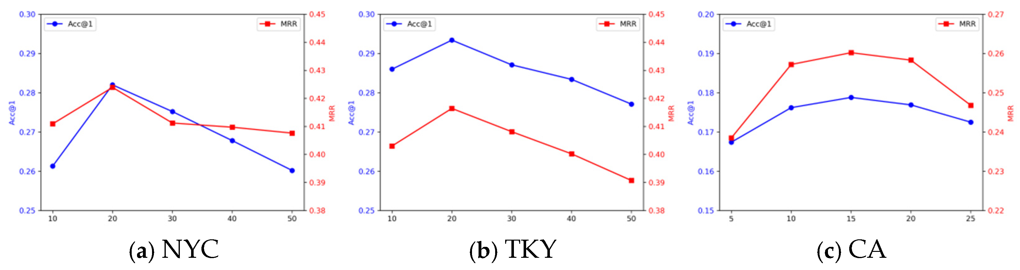
We perform a set of experiments on three public datasets and achieve superior performance in nearly all the comparison experiments. The experiments on different user behaviors show our model can be applied to different scenarios. Moreover, we analyze the effectiveness of our proposed meta-path-based methods. It shows comparable results compared with the results from the real-world data. The method is not a substitute for real-world data, but can be valid when users’ side information, like friendship, is missing. The ablation experiments confirm the effectiveness of our proposed components.

There are also some limitations in the research. We can focus on designing more effective contrastive learning methods to extract the most useful information from the graph, thereby directly improving the relevance to the downstream tasks. Additionally, the cold-start problem is vital in recommendation systems. Users or POIs without any check-ins can be great challenges when constructing heterogeneous graphs and meta-path-based subgraphs.

References

1. Rendle, S.; Freudenthaler, C.; Schmidt-Thieme, L. Factorizing personalized markov chains for next-basket recommendation. In Proceedings of the 19th International Conference on World Wide Web, Raleigh, NC, USA, 26–30 April 2010; pp. 811–820. [Google Scholar]
2. Lian, D.; Zhao, C.; Xie, X.; Sun, G.; Chen, E.; Rui, Y. GeoMF: Joint geographical modeling and matrix factorization for point-of-interest recommendation. In Proceedings of the 20th ACM SIGKDD International Conference on Knowledge Discovery and Data Mining, New York, NY, USA, 24–27August 2014; pp. 831–840. [Google Scholar]
3. He, J.; Li, X.; Liao, L.J. Category-aware Next Point-of-Interest Recommendation via Listwise Bayesian Personalized Ranking. In Proceedings of the 26th International Joint Conference on Artificial Intelligence (IJCAI), Melbourne, Australia, 19–25 August 2017; pp. 1837–1843. [Google Scholar]
4. Liu, W.; Wang, Z.J.; Yao, B.; Nie, M.D.; Wang, J.; Mao, R.; Yin, J. Geographical Relevance Model for Long Tail Point-of-Interest Recommendation. In Proceedings of the 23rd International Conference on Database Systems for Advanced Applications (DASFAA), Gold Coast, Australia, 21–24 May 2018; pp. 67–82. [Google Scholar]
5. Xu, Y.Y.; Li, X.F.; Li, J.; Wang, C.Z.; Gao, R.; Yu, Y.H. SSSER: Spatiotemporal Sequential and Social Embedding Rank for Successive Point-of-Interest Recommendation. IEEE Access 2019, 7, 156804–156823. [Google Scholar] [CrossRef]
6. Liu, Q.; Wu, S.; Wang, L.; Tan, T. Predicting the next location: A recurrent model with spatial and temporal contexts. In Proceedings of the 30th Association-for-the-Advancement-of-Artificial-Intelligence (AAAI) Conference on Artificial Intelligence, Phoenix, AZ, USA, 12–17 February 2016; pp. 194–200. [Google Scholar]
7. Sun, K.; Qian, T.; Chen, T.; Liang, Y.; Nguyen, Q.V.H.; Yin, H. Where to go next: Modeling long-and short-term user preferences for point-of-interest recommendation. In Proceedings of the 34th AAAI Conference on Artificial Intelligence, New York, NY, USA, 7–12 February 2020; pp. 214–221. [Google Scholar]
8. Feng, J.; Li, Y.; Zhang, C.; Sun, F.; Meng, F.; Guo, A.; Jin, D. Deepmove: Predicting human mobility with attentional recurrent networks. In Proceedings of the 27th World Wide Web (WWW) Conference, Lyon, France, 23–27 April 2018; pp. 1459–1468. [Google Scholar]
9. Lian, D.F.; Wu, Y.J.; Ge, Y.; Xie, X.; Chen, E.H. Geography-Aware Sequential Location Recommendation. In Proceedings of the 26th ACM SIGKDD International Conference on Knowledge Discovery and Data Mining (KDD), Electr Network, Virtual Event, 23–27 August 2020; pp. 2009–2019. [Google Scholar]
10. Xie, M.; Yin, H.; Wang, H.; Xu, F.; Chen, W.; Wang, S. Learning graph-based poi embedding for location-based recommendation. In Proceedings of the 25th ACM International on Conference on Information and Knowledge Management, Indianapolis, IN, USA, 24–28 October 2016; pp. 15–24. [Google Scholar]
11. Liu, B.; Qian, T.; Liu, B.; Hong, L.; You, Z.; Li, Y. Learning spatiotemporal-aware representation for POI recommendation. arXiv 2017, arXiv:1704.08853. [Google Scholar] [CrossRef]
12. Lin, Y.; Liu, Z.; Sun, M.; Liu, Y.; Zhu, X. Learning entity and relation embeddings for knowledge graph completion. In Proceedings of the AAAI Conference on Artificial Intelligence, Philadelphia, PA, USA, 25 February–4 March 2015. [Google Scholar]
13. Christoforidis, G.; Kefalas, P.; Papadopoulos, A.; Manolopoulos, Y. Recommendation of Points-of-Interest Using Graph Embeddings. In Proceedings of the 2018 IEEE 5th International Conference on Data Science and Advanced Analytics (DSAA), Turin, Italy, 1–3 October 2018. [Google Scholar]
14. You, Y.; Chen, T.; Sui, Y.; Chen, T.; Wang, Z.; Shen, Y. Graph contrastive learning with augmentations. Adv. Neural Inf. Process. Syst. 2020, 33, 5812–5823. [Google Scholar]
15. Yang, S.; Liu, J.; Zhao, K. GETNext: Trajectory flow map enhanced transformer for next POI recommendation. In Proceedings of the 45th International ACM SIGIR Conference on Research and Development in Information Retrieval, Madrid, Spain, 11–15 July 2022; pp. 1144–1153. [Google Scholar]
16. Yan, X.; Song, T.; Jiao, Y.; He, J.; Wang, J.; Li, R.; Chu, W. Spatio-temporal hypergraph learning for next POI recommendation. In Proceedings of the 46th international ACM SIGIR Conference on Research and Development in Information Retrieval, Taipei, Taiwan, 23–27 July 2023; pp. 403–412. [Google Scholar]
17. Qin, Y.F.; Wang, Y.F.; Sun, F.; Ju, W.; Hou, X.Y.; Wang, Z.; Cheng, J.; Lei, J.; Zhang, M. DisenPOI: Disentangling Sequential and Geographical Influence for Point-of-Interest Recommendation. In Proceedings of the 16th International Conference on Web Search and Data Mining, Singapore, 27 Feb–3 March 2023; pp. 508–516. [Google Scholar]
18. Wang, Z.B.; Zhu, Y.M.; Liu, H.B.; Wang, C.Y. Learning Graph-based Disentangled Representations for Next POI Recommendation. In Proceedings of the 45th International ACM SIGIR Conference on Research and Development in Information Retrieval (SIGIR), Madrid, Spain, 11–15 July 2022; pp. 1154–1163. [Google Scholar]
19. Wu, Y.; Li, K.; Zhao, G.; Qian, X. Long-and short-term preference learning for next POI recommendation. In Proceedings of the 28th ACM International Conference on Information and Knowledge Management, Beijing, China, 3–7 November 2019; pp. 2301–2304. [Google Scholar]
20. Wu, Y.; Li, K.; Zhao, G.; Qian, X. Personalized long-and short-term preference learning for next POI recommendation. IEEE Trans. Knowl. Data Eng. 2020, 34, 1944–1957. [Google Scholar] [CrossRef]
21. Zhao, P.; Luo, A.; Liu, Y.; Xu, J.; Li, Z.; Zhuang, F.; Sheng, V.S.; Zhou, X. Where to go next: A spatio-temporal gated network for next poi recommendation. IEEE Trans. Knowl. Data Eng. 2020, 34, 2512–2524. [Google Scholar] [CrossRef]
22. Luo, Y.; Liu, Q.; Liu, Z. Stan: Spatio-temporal attention network for next location recommendation. In Proceedings of the Web Conference 2021, Ljubljana, Slovenia, 19–23 April 2021; pp. 2177–2185. [Google Scholar]
23. Lim, N.; Hooi, B.; Ng, S.-K.; Goh, Y.L.; Weng, R.; Tan, R. Hierarchical multi-task graph recurrent network for next poi recommendation. In Proceedings of the 45th International ACM SIGIR Conference on Research and Development in Information Retrieval, Madrid, Spain, 11–15 July 2022; pp. 1133–1143. [Google Scholar]
24. Wang, D.; Chen, C.; Di, C.; Shu, M. Exploring Behavior Patterns for Next-POI Recommendation via Graph Self-Supervised Learning. Electronics 2023, 12, 1939. [Google Scholar] [CrossRef]
25. Fu, J.; Gao, R.; Yu, Y.; Wu, J.; Li, J.; Liu, D.; Ye, Z. Contrastive graph learning long and short-term interests for POI recommendation. Expert Syst. Appl. 2024, 238, 121931. [Google Scholar] [CrossRef]
26. Jiang, S.; He, W.; Cui, L.; Xu, Y.; Liu, L. Modeling Long- and Short-Term User Preferences via Self-Supervised Learning for Next POI Recommendation. ACM Trans. Knowl. Discov. Data 2023, 17, 1–20. [Google Scholar] [CrossRef]
27. Zhou, H.L.; Jia, Z.H.; Zhu, H.Y.; Zhang, Z.Z. CLLP: Contrastive Learning Framework Based on Latent Preferences for Next POI Recommendation. In Proceedings of the 47th Annual International ACM SIGIR Conference on Research and Development in Information Retrieval (SIGIR), Washington, DC, USA, 14–18 July 2024; pp. 1473–1482. [Google Scholar]
28. Wang, X.; Ji, H.; Shi, C.; Wang, B.; Ye, Y.; Cui, P.; Yu, P.S. Heterogeneous graph attention network. In Proceedings of the World Wide Web Conference, San Francisco, CA, USA, 13–17 May 2019; pp. 2022–2032. [Google Scholar]
29. Hu, Z.; Dong, Y.; Wang, K.; Sun, Y. Heterogeneous graph transformer. In Proceedings of the Web Conference 2020, Taipei, Taiwan, 20–24 April 2020; pp. 2704–2710. [Google Scholar]
30. Fu, X.; Zhang, J.; Meng, Z.; King, I. Magnn: Meta-path aggregated graph neural network for heterogeneous graph embedding. In Proceedings of the Web Conference 2020, Taipei, Taiwan, 20–24 April 2020; pp. 2331–2341. [Google Scholar]
31. Wang, X.; Liu, N.; Han, H.; Shi, C. Self-supervised heterogeneous graph neural network with co-contrastive learning. In Proceedings of the 27th ACM SIGKDD Conference on Knowledge Discovery & Data Mining, Virtual Event, 14–18 August 2021; pp. 1726–1736. [Google Scholar]
32. Wang, Z.; Li, Q.; Yu, D.; Han, X.; Gao, X.-Z.; Shen, S. Heterogeneous graph contrastive multi-view learning. In Proceedings of the 2023 SIAM International Conference on Data Mining (SDM), Twin Cities, MN, USA, 27–29 April 2023; pp. 136–144. [Google Scholar]
33. Tian, Y.; Dong, K.; Zhang, C.; Zhang, C.; Chawla, N.V. Heterogeneous graph masked autoencoders. In Proceedings of the AAAI Conference on Artificial Intelligence, Philadelphia, PA, USA, 25 February–4 March 2025; pp. 9997–10005. [Google Scholar]
34. Chen, M.; Huang, C.; Xia, L.; Wei, W.; Xu, Y.; Luo, R. Heterogeneous graph contrastive learning for recommendation. In Proceedings of the Sixteenth ACM International Conference on Web Search and Data Mining, Singapore, 27 February–3 March 2023; pp. 544–552. [Google Scholar]
35. Yu, J.X.; Ge, Q.Q.; Li, X.; Zhou, A.Y. Heterogeneous Graph Contrastive Learning With Meta-Path Contexts and Adaptively Weighted Negative Samples. IEEE Trans. Knowl. Data Eng. 2024, 36, 5181–5193. [Google Scholar] [CrossRef]
36. Xie, Y.Z.; Yu, C.Y.; Jin, X.Z.; Cheng, L.; Hu, B.; Li, Z. Heterogeneous graph contrastive learning for cold start cross-domain recommendation. Knowl.-Based Syst. 2024, 299, 112054. [Google Scholar] [CrossRef]
37. Huo, C.Y.; He, D.X.; Li, Y.W.; Jin, D.; Dang, J.W.; Pedrycz, W.; Wu, L.F.; Zhang, W.X. Heterogeneous Graph Neural Networks using Self-supervised Reciprocally Contrastive Learning. ACM Trans. Intell. Syst. Technol. 2025, 16, 1–21. [Google Scholar] [CrossRef]
38. Bai, W.H.; Qiu, L.Q.; Zhao, W.D. Dynamic heterogeneous graph contrastive learning based on multi-prior tasks. Neurocomputing 2025, 647, 130612. [Google Scholar] [CrossRef]
39. Moradi, M.; Moradi, P.; Faroughi, A.; Jalili, M. Two-level attention mechanism with contrastive learning for heterogeneous graph representation learning. Expert Syst. Appl. 2025, 273, 126751. [Google Scholar] [CrossRef]
40. Chen, Y.; Wu, L.; Zaki, M. Iterative deep graph learning for graph neural networks: Better and robust node embeddings. Adv. Neural Inf. Process. Syst. 2020, 33, 19314–19326. [Google Scholar]
41. Li, R.; Wang, S.; Zhu, F.; Huang, J. Adaptive graph convolutional neural networks. arXiv 2018, arXiv:1801.03226. [Google Scholar] [CrossRef]
42. Wang, X.; Zhu, M.; Bo, D.; Cui, P.; Shi, C.; Pei, J. AM-GCN: Adaptive multi-channel graph convolutional networks. In Proceedings of the 26th ACM SIGKDD International Conference on Knowledge Discovery & Data Mining, Virtual Event, CA, USA, 6–10 July 2020; pp. 1243–1253. [Google Scholar]
43. Franceschi, L.; Niepert, M.; Pontil, M.; He, X. Learning discrete structures for graph neural networks. In Proceedings of the International Conference on Machine Learning, Long Beach, CA, USA, 9–15 June 2019; pp. 1972–1982. [Google Scholar]
44. Luo, D.; Cheng, W.; Yu, W.; Zong, B.; Ni, J.; Chen, H.; Zhang, X. Learning to drop: Robust graph neural network via topological denoising. In Proceedings of the 14th ACM International Conference on Web Search and Data Mining, Virtual Event, 8–12 March 2021; pp. 779–787. [Google Scholar]
45. Zheng, C.; Zong, B.; Cheng, W.; Song, D.; Ni, J.; Yu, W.; Chen, H.; Wang, W. Robust graph representation learning via neural sparsification. Proc. Int. Conf. Mach. Learn. 2020, 119, 11458–11468. [Google Scholar]
46. Gao, X.; Hu, W.; Guo, Z. Exploring structure-adaptive graph learning for robust semi-supervised classification. In Proceedings of the 2020 IEEE International Conference on Multimedia and Expo (ICME), London, UK, 6–10 July 2020; pp. 1–6. [Google Scholar]
47. Jin, W.; Ma, Y.; Liu, X.; Tang, X.; Wang, S.; Tang, J. Graph structure learning for robust graph neural networks. In Proceedings of the 26th ACM SIGKDD International Conference on Knowledge Discovery & Data Mining, Virtual Event, 6–10 July 2020; pp. 66–74. [Google Scholar]
48. Yang, L.; Kang, Z.; Cao, X.; Jin, D.; Yang, B.; Guo, Y. Topology Optimization based Graph Convolutional Network. In Proceedings of the Twenty-Eighth International Joint Conference on Artificial Intelligence (IJCAI-19), Macao, China, 10–16 August 2019; pp. 4054–4061. [Google Scholar]
49. Jia, N.; Tian, X.L.; Yang, T.; Li, S.; Jiao, L.C. Self-restrained contrastive enhanced network for graph structure learning. Expert Syst. Appl. 2024, 249, 123520. [Google Scholar] [CrossRef]
50. Wang, L.; Wu, S.; Liu, Q.; Zhu, Y.Q.; Tao, X.; Zhang, M.D.; Wang, L. Bi-Level Graph Structure Learning for Next POI Recommendation. IEEE Trans. Knowl. Data Eng. 2024, 36, 5695–5708. [Google Scholar] [CrossRef]
51. Xie, X.T.; Chen, W.Y.; Kang, Z. Robust graph structure learning under heterophily. Neural Netw. 2025, 185, 107206. [Google Scholar] [CrossRef]
52. Yu, J.; Yin, H.; Li, J.; Wang, Q.; Hung, N.Q.V.; Zhang, X. Self-supervised multi-channel hypergraph convolutional network for social recommendation. In Proceedings of the Web Conference 2021, Ljubljana, Slovenia, 19–23 April 2021; pp. 413–424. [Google Scholar]
53. Xu, K.; Hu, W.; Leskovec, J.; Jegelka, S. How powerful are graph neural networks? arXiv 2018, arXiv:1810.00826. [Google Scholar]
54. He, X.; Deng, K.; Wang, X.; Li, Y.; Zhang, Y.; Wang, M. Lightgcn: Simplifying and powering graph convolution network for recommendation. In Proceedings of the 43rd International ACM SIGIR Conference on Research and Development in Information Retrieval, Virtual Event, 25–30 July 2020; pp. 639–648. [Google Scholar]
55. Hochreiter, S.; Schmidhuber, J. Long short-term memory. Neural Comput. 1997, 9, 1735–1780. [Google Scholar] [CrossRef] [PubMed]
56. Feng, S.; Li, X.; Zeng, Y.; Cong, G.; Chee, Y.; Yuan, Q. Personalized Ranking Metric Embedding for next New POI Recommendation. In Proceedings of the 24th International Conference on Artificial Intelligence (IJCAI’15), Buenos Aires, Argentina, 25–31 July 2015; pp. 2069–2075. [Google Scholar]
Figure 1. Overview of HGSL-POI.
Algorithms 18 00478 g001
Figure 2. A specific schematic diagram of heterogeneous graph contrastive learning: (a) Meta-path based Contrastive Learning, and (b) Interaction-Aware Contrastive Learning.
Algorithms 18 00478 g002
Figure 3. A schematic diagram of sequence modeling.
Algorithms 18 00478 g003
Figure 4. Different number of sequences of the same user on different datasets.
Algorithms 18 00478 g004
Figure 5. Number of different sequences of different users on different datasets.
Algorithms 18 00478 g005
Figure 6. Performance of the model under different embedding dimensions.
Algorithms 18 00478 g006
Figure 7. Performance of the model under different add/removal ratios.
Algorithms 18 00478 g007