Fractional Discrete Computer Virus System: Chaos and Complexity Algorithms

Abstract

The spread of computer viruses represents a major challenge to digital security, underscoring the need for a deeper understanding of their propagation mechanisms. This study examines the stability and chaotic dynamics of a fractional discrete Susceptible-Infected (SI) model for computer viruses, incorporating commensurate and incommensurate types of fractional orders. Using the basic reproduction number $R_0$, the derivation of stability conditions is followed by an investigation of how varying fractional orders affect the system’s behavior. To explore the system’s nonlinear chaotic behavior, the research of this study employs a suite of analytical tools, including the analysis of bifurcation diagrams, phase portraits, and the evaluation of the maximum Lyapunov exponent (MLE) for the study of chaos. The model’s complexity is confirmed through advanced complexity algorithms, including spectral entropy, approximate entropy, and the $0-1$ test. These measures offer a more profound insight into the complex behavior of the system and the role of fractional order. Numerical simulations provide visual evidence of the distinct dynamics associated with commensurate and incommensurate fractional orders. These results provide insights into how fractional derivatives influence behaviors in cyberspace, which can be leveraged to design enhanced cybersecurity measures.

1. Introduction

Computer viruses represent a significant and ever-growing threat to cybersecurity in an increasingly digital world. These malicious programs are designed to self-replicate, spreading from one system to another by attaching themselves to legitimate files or software. Unlike different types of malware, such as worms or Trojans, viruses typically require some form of user interaction to execute and begin their propagation [1,2]. The consequences of a virus infection can be devastating, ranging from the corruption and loss of critical data and system failures to substantial financial losses, widespread operational disruption, and severe breaches of privacy [3,4]. In today’s interconnected world, the impact of a successful virus attack can ripple outward, affecting individuals, organizations, and even critical infrastructure. The evolution of computer viruses has been marked by a steady increase in complexity and sophistication. Early viruses, such as the Creeper program of the 1970s, were relatively harmless, often serving as experimental projects [5]. However, these early examples quickly gave way to more malicious creations. Notable viruses like Stuxnet demonstrated the potential for viruses to inflict massive economic damage and even target critical infrastructure, highlighting the real-world consequences of these digital threats [6]. Modern viruses employ increasingly sophisticated techniques to evade detection and maintain persistence within digital environments. For example, polymorphic and metamorphic viruses dynamically alter their code, making it extremely difficult for traditional signature-based detection systems to identify and neutralize them [7]. This constant evolution necessitates a continuous adaptation of cybersecurity defense mechanisms.

In the ongoing battle against computer viruses, studies have turned to mathematical modeling as a critical tool for understanding virus propagation and developing effective containment strategies [8]. Drawing inspiration from biological epidemiology, various methods have been adapted from traditional epidemic models to analyze and predict the spread of viruses within computer networks [9]. Among these, the Susceptible-Infected (SI) model is a widely used framework for examining virus behavior. However, the standard integer-order versions of these models often fall short when attempting to capture long-term dependencies and memory effects frequently observed in real-world cyber threats [10]. Standard models frequently employ simplifications of intricate interactions and fail to account for the historical context of virus spread. This limitation has led to a growing interest in fractional-order models, which incorporate historical interactions and offer a more detailed and precise depiction of virus propagation [11]. By integrating memory effects, fractional-order models offer a more realistic and powerful tool for predicting and mitigating the impact of evolving digital threats. In parallel, some studies have analyzed the spread of actual computer viruses such as Code Red, Slammer, Conficker, and Stuxnet, using parameterized statistical distributions to fit real outbreak data [12]. These works provide a valuable benchmark for validating the qualitative behavior of theoretical models, including those based on fractional calculus.

Fractional calculus, extending classical calculus, extends differentiation and integration concepts to non-integer orders. This mathematical framework offers unique advantages for modeling complex systems by incorporating memory effects and hereditary properties [13]. Unlike traditional integer-order derivatives, which analyze only local changes, fractional derivatives consider the influence of past events on the present and future behavior of a system [14]. This property makes fractional calculus highly effective in studying systems with long-term dependencies, such as the spread of viruses in digital networks [15]. The application of fractional calculus in mathematical modeling has gained traction within a diverse range of fields, notably physics, biology, engineering, and finance [16]. In epidemiology and cybersecurity, fractional models have been particularly successful in capturing the history-dependent nature of disease and virus propagation [17]. By incorporating fractional derivatives, it is possible to better understand how past infections influence current and future outbreaks, leading to more accurate predictive models [18]. In discrete systems, fractional calculus provides a robust framework for analyzing systems that evolve in discrete time steps, making it highly suitable for modeling digital networks and computational processes. Unlike continuous-time models, which may not fully capture digital environments’ complexities, discrete fractional models offer a more precise approach to studying virus spread in cyberspace. These models account for the cumulative impact of previous infections, providing valuable insights into how viruses persist, adapt, and evolve over time [19].

A fractional discrete SI model extends the classical SI model by incorporating fractional-order derivatives to capture long-term dependencies in virus transmission. While traditional SI models assume that the rate of infection relies solely on the information contained in the current system state, the fractional framework considers historical infection trends, leading to a more accurate representation of real-world virus behavior [20]. The utilization of discrete fractional models in cybersecurity makes it possible to identify hidden patterns, predict outbreaks, and develop proactive defense mechanisms [21]. By analyzing the system’s dynamics, one can determine the conditions under which a virus persists, dies out, or exhibits chaotic behavior [22]. This insight is crucial for designing effective cybersecurity policies, intrusion detection systems, and digital defense strategies. Furthermore, nonlinear analysis, particularly bifurcation theory, is key to understanding the critical points where small changes in system parameters can lead to drastic shifts in behavior, such as the transition from stable infection dynamics to chaotic outbreaks. This allows for a more detailed exploration of how digital epidemics evolve and how they may be controlled or mitigated.

This research investigates the stability and chaotic dynamics of a susceptible-infected (SI) model for computer virus propagation with fractional discrete dynamics, using the Caputo-like difference operator. The key motivation behind this work lies in the growing challenge of controlling sophisticated computer viruses whose spread exhibits unpredictable and highly sensitive dynamics. Understanding such chaotic behavior is essential for designing robust and adaptive cybersecurity strategies. In this context, fractional calculus offers a powerful framework for modeling long-term dependencies and capturing non-local behavior that classical models may overlook. When a virus exhibits chaotic behavior, even minor variations in initial conditions can lead to drastically different outcomes, making prediction and control significantly more difficult. This study provides an in-depth analysis of the relationship between fractional calculus and chaotic dynamics, contributing to the development of more resilient digital defense mechanisms. Unlike normalized continuous-time fractional SIR models [23], which use the Caputo derivative, our model employs a discrete-time Caputo-like fractional difference operator. This approach is more appropriate for modeling digital systems like computer virus spread, where interactions naturally occur at discrete time intervals. The novelty of our work lies in constructing a fractional discrete SI model with both commensurate and incommensurate fractional orders and uncovering its chaotic behavior using advanced nonlinear tools. To the best of our knowledge, our model is the first to explore chaotic dynamics in a discrete fractional SI framework with both commensurate and incommensurate orders. This analysis enables a deeper understanding of virus dynamics and offers insights for designing more robust cybersecurity mechanisms.

The main contributions of this work are as follows:

• We derive the stability conditions of the proposed fractional discrete SI model using the basic reproduction number $R_0$, which helps predict whether a virus outbreak will persist or die out.
• We examine the influence of both commensurate and incommensurate fractional orders on the system’s dynamics, emphasizing their ability to capture memory effects in digital virus propagation.
• We apply several chaos detection and complexity analysis tools, including bifurcation diagrams, phase portraits, maximum Lyapunov exponents, spectral entropy, approximate entropy, and the $0-1$ test for chaos, to reveal nonlinear and chaotic behaviors in the model.
• We demonstrate through extensive numerical simulations that the model can exhibit chaos under specific parameter values, revealing the complex and unpredictable nature of virus spread in cyberspace.

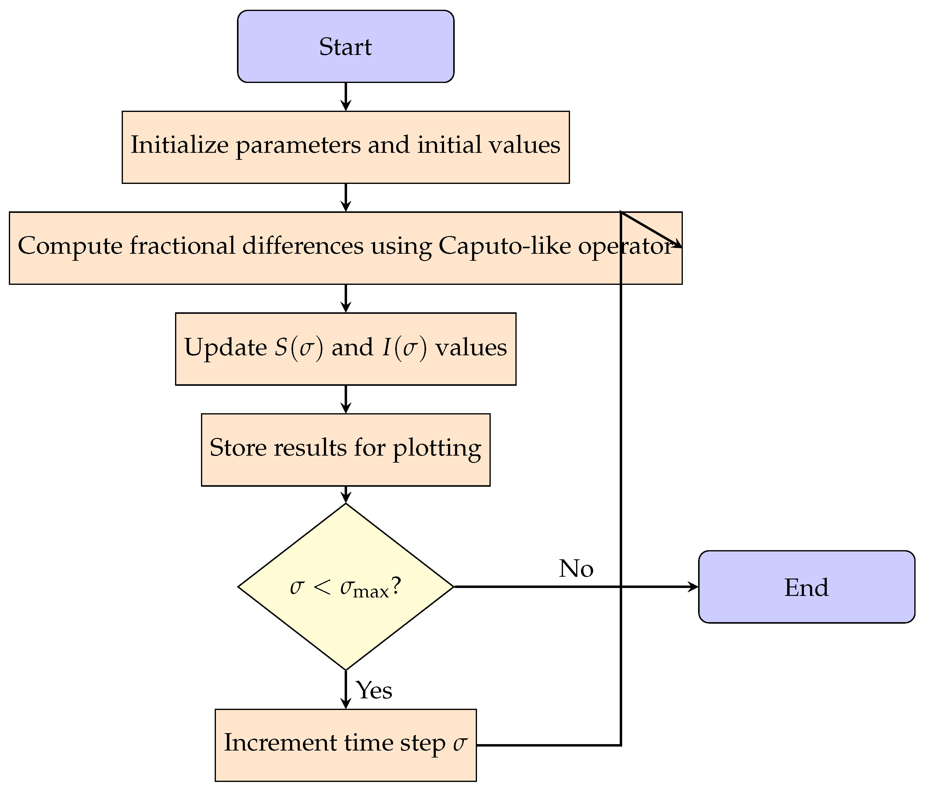
The research in this study begins in Section 2 by establishing the necessary background on fractional calculus in discrete time and deriving the Caputo-like fractional discrete computer virus model. Section 3 then focuses on the model under commensurate and incommensurate fractional orders, analyzing its equilibrium points and their stability. Dynamical analysis and simulation results of the fractional model are considered in Section 4. 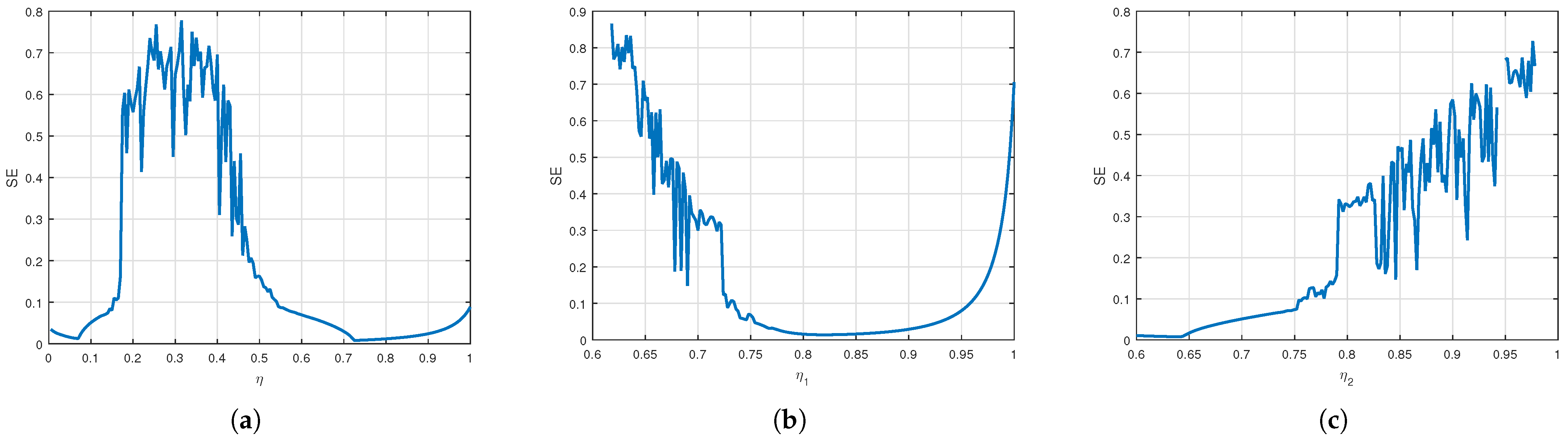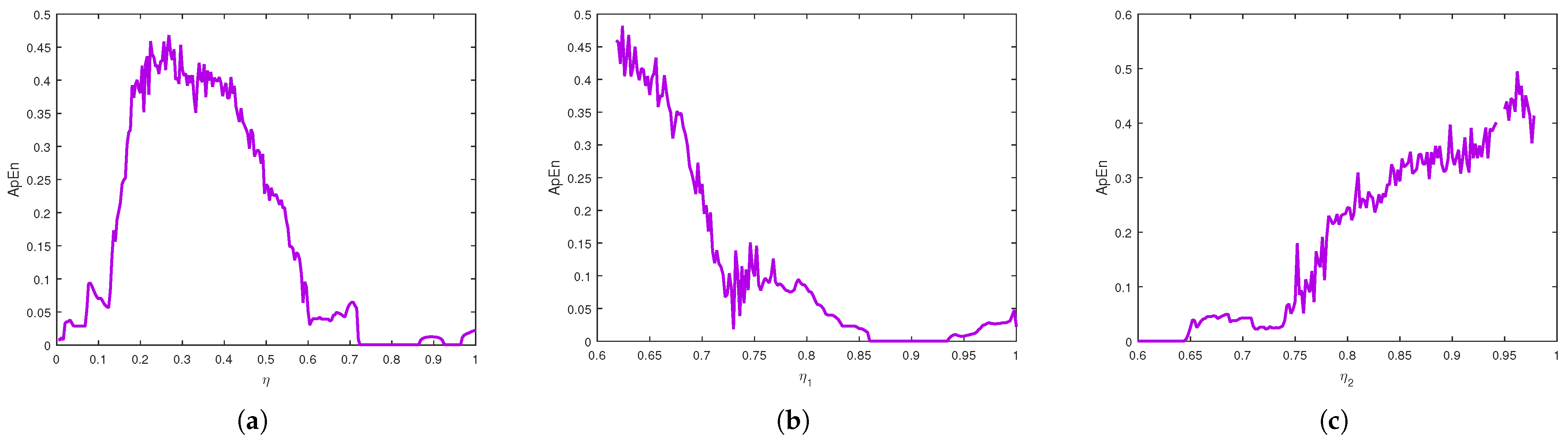Section 5 explores the complexity of chaos using the SE complexity algorithm, approximate entropy, and the $0-1$ test. The paper concludes in Section 6, summarizing key results and outlining future work.

2. Theoretical Foundations and Model Description

This section is introduced with two subsections. The first provides essential background on discrete fractional calculus, while the second presents a detailed description of the proposed model.

2.1. Theoretical Foundations

Before constructing the fractional-order Computer Virus Model, a necessary introduction is provided by means of discrete fractional calculus. Specifically, the Caputo-like difference operator is introduced, that is, ${}^c\Delta _{\rho }^{\eta }$ from [24], which will be central to the derivation and subsequent analysis of the fractional model.

The Caputo-like difference operator, ${}^c\Delta _{\rho }^{\eta }$, is defined as

$${}^c\Delta _{\rho }^{\eta }\chi \left(\sigma \right)={\Delta }_{\rho }^{-(\alpha -\eta )}{\Delta }^{\alpha }\chi \left(\sigma \right),$$

(1)

such as $\sigma \in {\mathbb{N}}_{\rho +\alpha -\eta }$, and $\alpha =\lceil \eta \rceil +1$. The fractional sum ${\Delta }_{\rho }^{-\eta }$ is defined in [25] as

$${\Delta }_{\rho }^{-\eta }\chi \left(\sigma \right)={\displaystyle \frac{1}{\mathrm{\Gamma }\left(\eta \right)}}\sum _{\varsigma =\eta }^{\sigma -\eta }{(\sigma -1-\varsigma )}^{(\eta -1)}\chi \left(\varsigma \right).$$

(2)

Theorem 1

([26]). Regarding the delta fractional difference equation

$$\left\{\begin{array}{c}{}^c\Delta _{\rho }^{\eta }\chi \left(\sigma \right)=g(\sigma +\eta -1,\chi (\sigma +\eta -1)),\hfill \\ {\Delta }^j\chi \left(\rho \right)={\chi }_j,\alpha =\lceil \eta \rceil +1,j=0,\dots ,\alpha -1.\hfill \end{array}\right.$$

(3)

The corresponding integral equation in the discrete domain can be formulated as

$$\chi \left(\sigma \right)={\chi }_0\left(\sigma \right)+{\displaystyle \frac{1}{\mathrm{\Gamma }\left(\eta \right)}}\sum _{\varsigma =\rho +\alpha -\eta }^{\sigma -\eta }{(\sigma -\varsigma -1)}^{(\eta -1)}g(\sigma +\eta -1,\chi (\sigma +\eta -1)),\sigma \in {\mathbb{N}}_{\rho +\alpha },$$

(4)

in which the initial iteration ${\chi }_0\left(\sigma \right)$ takes the form

$${\chi }_0\left(\sigma \right)=\sum _{j=0}^{\alpha -1}{\displaystyle \frac{{(\sigma -\rho )}^j}{\mathrm{\Gamma }(j+1)}}{\Delta }^j\chi \left(\rho \right).$$

(5)

When $\rho =0$, $\alpha =1$, $j=\varsigma +\eta -1$, and

$${(\sigma -1-\varsigma )}^{(\eta -1)}={\displaystyle \frac{\mathrm{\Gamma }(\sigma -\varsigma )}{\mathrm{\Gamma }(\sigma -\varsigma -\eta +1)}},$$

(6)

for $\eta \in (0,1]$, the above Equation (4) is numerically formulated as

$$\chi \left(\sigma \right)=\chi \left(0\right)+{\displaystyle \frac{1}{\mathrm{\Gamma }\left(\eta \right)}}\sum _{j=0}^{\sigma -1}{\displaystyle \frac{\mathrm{\Gamma }(\sigma -1+\eta -j)}{\mathrm{\Gamma }(\sigma -j)}}g(j,\chi \left(j\right)).$$

(7)

2.2. Model Description

The model considers three distinct states for computers within the network: susceptible (S(t)), infected (I(t)), and recovered (R(t)), based on [27,28,29,30]. Four parameters govern the transitions between these states: b (the rate of new computers joining), $ϵ$ (recovery rate), d (removal rate), and $\lambda$ (the infection rate).

$$\left\{\begin{array}{c}{\displaystyle \frac{dS}{dt}}=b-\lambda S\left(t\right)I\left(t\right)-dS\left(t\right),\hfill \\ {\displaystyle \frac{dI}{dt}}=\lambda S\left(t\right)I\left(t\right)-ϵI\left(t\right)-dI\left(t\right),\hfill \\ {\displaystyle \frac{dR}{dt}}=ϵI\left(t\right)-dR\left(t\right).\hfill \end{array}\right.$$

(8)

It is noteworthy that the recovered compartment R in System (8) exhibits no influence on the dynamics of the susceptible or infected compartments. Consequently, this study will be restricted to the following reduced system:

$$\left\{\begin{array}{c}{\displaystyle \frac{dS}{dt}}=b-\lambda S\left(t\right)I\left(t\right)-dS\left(t\right),\hfill \\ {\displaystyle \frac{dI}{dt}}=\lambda S\left(t\right)I\left(t\right)-ϵI\left(t\right)-dI\left(t\right).\hfill \end{array}\right.$$

(9)

The discretization and dynamical analysis in this work are based on model (9). This choice is motivated by the discrete nature of real-world data, which makes discrete models more suitable for simulating virus transmission. To obtain a discrete approximation of model (9), the forward Euler scheme with a unit time step is employed, yielding

$$\left\{\begin{array}{c}S(\sigma +1)=b-\lambda S\left(\sigma \right)I\left(\sigma \right)-dS\left(\sigma \right)+S\left(\sigma \right),\hfill \\ I(\sigma +1)=\lambda S\left(\sigma \right)I\left(\sigma \right)-ϵI\left(\sigma \right)-dI\left(\sigma \right)+I\left(\sigma \right).\hfill \end{array}\right.$$

(10)

Equation (10) provides a discrete-time approximation using the forward Euler method. This scheme is widely adopted due to its simplicity and effectiveness in digital simulations. The validity of this discretization is supported by its ability to preserve essential qualitative features of the continuous model, such as stability and positivity of solutions. Additionally, the accuracy of this method has been verified through extensive simulations and alignment with theoretical predictions. Convergence results for similar discrete schemes can be found in [24,25], further supporting the reliability of the adopted approach.

To highlight the dynamics in the first-order difference setting, we also present the classical discrete SI model as

$$\left\{\begin{array}{c}\Delta S\left(\sigma \right)=b-\lambda S\left(\sigma \right)I\left(\sigma \right)-dS\left(\sigma \right),\hfill \\ \Delta I\left(\sigma \right)=\lambda S\left(\sigma \right)I\left(\sigma \right)-ϵI\left(\sigma \right)-dI\left(\sigma \right).\hfill \end{array}\right.$$

(11)

In light of the preceding considerations, attention is now turned to the analysis of the following discrete-time fractional model for the propagation of computer viruses using the Caputo-like difference operator:

$$\left\{\begin{array}{c}{}^c\Delta _{\rho }^{\eta }S\left(\sigma \right)=b-\lambda S(\sigma +\eta -1)I(\sigma +\eta -1)-dS(\sigma +\eta -1),\hfill \\ {}^c\Delta _{\rho }^{\eta }I\left(\sigma \right)=\lambda S(\sigma +\eta -1)I(\sigma +\eta -1)-ϵI(\sigma +\eta -1)-dI(\sigma +\eta -1).\hfill \end{array}\right.$$

(12)

where ${}^c\Delta _{\rho }^{\eta }$ denotes the Caputo-like discrete fractional difference operator of order $\eta$ with base point $\rho$.

3. Stability Analysis of Equilibria

Here, an analysis is carried out to assess the stability and dynamics of the fractional discrete computer virus system (12) under commensurate and incommensurate orders.

Setting $\rho =0$ and applying Theorem 1, the fractional discrete model’s numerical Formula (12) is

$$\left\{\begin{array}{c}S\left(\sigma \right)=S\left(0\right)+{\displaystyle \frac{1}{\mathrm{\Gamma }\left(\eta \right)}}\sum _{j=1}^{\sigma }{\displaystyle \frac{\mathrm{\Gamma }(\sigma -j+\eta )}{\mathrm{\Gamma }(\sigma -j+1)}}[b-\lambda S(j-1)I(j-1)-dS(j-1)],\hfill \\ I\left(\sigma \right)=I\left(0\right)+{\displaystyle \frac{1}{\mathrm{\Gamma }\left(\eta \right)}}\sum _{j=1}^{\sigma }{\displaystyle \frac{\mathrm{\Gamma }(\sigma -j+\eta )}{\mathrm{\Gamma }(\sigma -j+1)}}[\lambda S(j-1)I(j-1)-ϵI(j-1)-dI(j-1)].\end{array}\right.$$

(13)

A crucial step in analyzing the dynamics of System (12) is determining its fixed points. To achieve this, it is necessary to solve the following nonlinear system:

$$\left\{\begin{array}{c}b-\lambda SI-dS=0,\hfill \\ \lambda SI-ϵI-dI=0.\hfill \end{array}\right.$$

(14)

Equation (14) has a virus-free equilibrium $E_0=({\displaystyle \frac{b}{d}},0)$ and a positive solution $E_{*}=({\displaystyle \frac{ϵ+d}{\lambda }},{\displaystyle \frac{b}{ϵ+d}}-{\displaystyle \frac{d}{\lambda }})$.

$R_0$, identified as the basic reproduction number, is a fundamental epidemiological parameter that denotes the mean measure of new infections attributable to a single infective in a population of susceptible individuals. In the context of computer virus propagation, $R_0$ can be thought of as the average number of devices or systems that a single infected device will successfully compromise within a fully vulnerable network. An $R_0$ value greater than 1 indicates the potential for a virus to spread throughout the network, while a value less than 1 suggests that the virus is unlikely to propagate. $R_0$ is calculated using the dominant eigenvalue of the next-generation matrix ${\mathcal{FV}}^{-1}$, as described in [31], where

$$\mathcal{F}=\left(\begin{array}{cc}0& 0\\ 0& {\displaystyle \frac{\lambda b}{d}}\end{array}\right),\mathrm{and}\mathcal{V}=\left(\begin{array}{cc}d& {\displaystyle \frac{\lambda b}{d}}\\ 0& ϵ+d\end{array}\right),$$

(15)

so

$${\mathcal{FV}}^{-1}=\left(\begin{array}{cc}0& 0\\ 0& {\displaystyle \frac{\lambda b}{d(ϵ+d)}}\end{array}\right).$$

(16)

Calculating the eigenvalues of ${\mathcal{FV}}^{-1}$ yields the reproduction number

$$R_0={\displaystyle \frac{\lambda b}{d(ϵ+d)}},$$

(17)

which implies $S_{*}={\displaystyle \frac{b}{d{R}_0}}$ and $I_{*}={\displaystyle \frac{d}{\lambda }}(R_0-1).$

3.1. The Commensurate Case

The next step is to establish sufficient conditions regarding the long-term stability of the two fixed points of System (12). Prior to examining stability, the following theorem is needed:

Theorem 2

([32]). Take into account the fractional difference system

$${}^c\Delta _{\rho }^{\eta }\chi \left(\sigma \right)=\mathcal{G}\chi (\sigma +\eta -1),$$

(18)

where $\chi \left(\sigma \right)={({\chi }_1\left(\sigma \right),\dots ,{\chi }_n\left(\sigma \right))}^T,0<\eta <1$, and ${\gamma }_j,(j=1,2,\dots ,n),$ are the eigenvalues of $\mathcal{G}\in {\mathbb{R}}^{n\times n}$. If all ${\gamma }_j,$ fulfill this condition

$${\gamma }_j,\in \left\{\vartheta \in \mathbb{C}:\left|\vartheta \right|<{\left(2cos{\displaystyle \frac{|arg(\vartheta \left)\right|-\pi }{2-\eta }}\right)}^{\eta },and|arg\left(\vartheta \right)|>{\displaystyle \frac{\eta \pi }{2}}\right\},$$

(19)

then the asymptotic stability of the zero solution of (18) is achieved.

The zero equilibrium point’s stability in fractional discrete maps is able to be assessed following Theorem 2. However, for non-zero equilibrium points, a distinct approach is necessary. To this end, the following change of variables is considered.

$$\left\{\begin{array}{c}{X}_0(\sigma +\eta -1)=S(\sigma +\eta -1)-S_0,Y_0(\sigma +\eta -1)=I(\sigma +\eta -1)-I_0,\hfill \\ X_{*}(\sigma +\eta -1)=S(\sigma +\eta -1)-S_{*},Y_{*}(\sigma +\eta -1)=I(\sigma +\eta -1)-I_{*}.\hfill \end{array}\right.$$

(20)

The transformation yields two new maps, both of which have a zero equilibrium

$$\left\{\begin{array}{cc}{}^c\Delta _{\rho }^{\eta }(X_0\left(\sigma \right)+S_0)\hfill & =b-\lambda (X_0(\sigma +\eta -1)+{\displaystyle \frac{b}{d}})Y_0(\sigma +\eta -1)-d(X_0(\sigma +\eta -1)+{\displaystyle \frac{b}{d}}),\hfill \\ {}^c\Delta _{\rho }^{\eta }(Y_0\left(\sigma \right)+I_0)\hfill & =\lambda (X_0(\sigma +\eta -1)+{\displaystyle \frac{b}{d}})Y_0(\sigma +\eta -1)-ϵY_0(\sigma +\eta -1)-d{Y}_0(\sigma +\eta -1),\hfill \end{array}\right.$$

(21)

and

$$\left\{\begin{array}{c}{}^c\Delta _{\rho }^{\eta }(X_{*}\left(\sigma \right)+S_{*})=b-\lambda (X_{*}(\sigma +\eta -1)+S_{*})(Y_{*}(\sigma +\eta -1)+I_{*})-d(X_{*}(\sigma +\eta -1)+S_{*}),\hfill \\ {}^c\Delta _{\rho }^{\eta }(Y_{*}\left(\sigma \right)+I_{*})=\lambda (X_{*}(\sigma +\eta -1)+S_{*})(Y_{*}(\sigma +\eta -1)+I_{*})-ϵ(Y_{*}(\sigma +\eta -1)+I_{*})-d(Y_{*}(\sigma +\eta -1)+I_{*}).\hfill \end{array}\right.$$

(22)

Proposition 1.

The virus-free fixed point, denoted $E_0$, of Model (12) is shown to be stable in a local asymptotic sense if the conditions outlined below are verified

$$d<2^{\eta },R_0<1,\left|(ϵ+d)(R_0-1)\right|<2^{\eta },$$

(23)

Proof. 

Determining the Jacobian matrix for model (21) at the zero equilibrium point yields

$${\mathcal{J}}_0=\left(\begin{array}{cc}-d& -{\displaystyle \frac{\lambda b}{d}}\\ 0& {\displaystyle \frac{\lambda b}{d}}-ϵ-d\end{array}\right),$$

(24)

the corresponding characteristic equation:

$$(-d-\gamma )\left({\displaystyle \frac{\lambda b}{d}}-ϵ-d-\gamma \right)=0,$$

(25)

the eigenvalues of ${\mathcal{J}}_0$ are ${\gamma }_1=-d$ and ${\gamma }_2={\displaystyle \frac{\lambda b}{d}}-ϵ-d=(ϵ+d)(R_0-1)$.

For ${\gamma }_1=-d$

$$\left\{\begin{array}{c}|{\gamma }_1|=d,\hfill \\ |arg{\gamma }_1|=\pi >{\displaystyle \frac{\kappa \pi }{2}},\hfill \end{array}\right.$$

(26)

the condition $|{\gamma }_1|<{\left(2cos{\displaystyle \frac{|arg{\gamma }_1|-\pi }{2-\eta }}\right)}^{\eta }=2^{\eta }$ is satisfied if $d<2^{\eta }$.

For ${\gamma }_2=(ϵ+d)(R_0-1)$

$$\left\{\begin{array}{c}|{\gamma }_2|=|(ϵ+d)(R_0-1)|,\hfill \\ |arg{\gamma }_2|=\pi ,\hfill \end{array}\right.$$

(27)

the condition $|{\gamma }_2|<{\left(2cos{\displaystyle \frac{|arg{\gamma }_2|-\pi }{2-\eta }}\right)}^{\eta }=2^{\eta }$ is satisfied if $|(ϵ+d)(R_0-1)|<2^{\eta }$, the condition $|arg{\gamma }_2|>{\displaystyle \frac{\kappa \pi }{2}}$, is satisfied if ${\gamma }_2<0$ i.e., $R_0<1$.

So the hypothesis of Theorem 13 is satisfied; the virus-free fixed point of (12) reveals local asymptotic stability. □

Proposition 2.

Local asymptotic stability of $E_{*}$ is guaranteed if either one of the following two conditions is verified.

$$A^2\ge 4B,R_0>1,|{\displaystyle \frac{-A\pm \sqrt{A^2-4B}}{2}}|<2^{\eta },$$

(28)

or

$$A^2<4B,|{\gamma }_{3,4}|<{\left(2cos{\displaystyle \frac{|arg{\gamma }_{3,4}|-\pi }{2-\eta }}\right)}^{\eta },|arg{\gamma }_{3,4}|>\eta {\displaystyle \frac{\pi }{2}}.$$

(29)

where $A={\displaystyle \frac{R_0}{d}}$ and $B=\lambda b(1-{\displaystyle \frac{1}{R_0}}).$

Proof. 

The Jacobian matrix is computed

$${\mathcal{J}}^{*}=\left(\begin{array}{cc}-\lambda I_{*}-d& -\lambda S_{*}\\ \lambda I_{*}& \lambda S_{*}-ϵ-d\end{array}\right),$$

(30)

The characteristic equation determines the eigenvalues of ${\mathcal{J}}^{*}$

$${\gamma }^2+A\gamma +B=0,$$

(31)

with

$$A={\displaystyle \frac{R_0}{d}}\mathrm{and}B=\lambda b(1-{\displaystyle \frac{1}{R_0}}),$$

(32)

which implies

$${\gamma }_{3,4}={\displaystyle \frac{1}{2}}\left(-A\pm \sqrt{A^2-4B}\right),$$

(33)

for $A^2\ge 4B$ The eigenvalues ${\gamma }_{3,4}$ have arguments of $\pi$ when ${\gamma }_{3,4}<0$ which is fulfilled if

$$\left\{\begin{array}{c}{\displaystyle \frac{R_0}{d}}>0,(\mathrm{holds}\mathrm{true}\mathrm{because}\mathrm{all}\mathrm{the}\mathrm{parameters}\mathrm{are}\mathrm{positive})\hfill \\ \lambda b(1-{\displaystyle \frac{1}{R_0}})>0,\mathrm{i}.\mathrm{e},R_0>1,\hfill \end{array}\right.$$

(34)

this leads to ${\gamma }_{3,4}=\pi >{\displaystyle \frac{\eta \pi }{2}}$. The condition $|{\gamma }_{3,4}|<{\left(2cos{\displaystyle \frac{|arg{\gamma }_{3,4}|-\pi }{2-\eta }}\right)}^{\eta }=2^{\eta }$ is valid if $|{\displaystyle \frac{-A\pm \sqrt{A^2-4B}}{2}}|<2^{\eta }$.

For $A^2<4B$, in this case, ${\gamma }_{3,4}$ are complex. The requirements for stability hold true if

$$|{\gamma }_{3,4}|<{\left(2cos{\displaystyle \frac{|arg({\gamma }_{3,4}\left)\right|-\pi }{2-\eta }}\right)}^{\eta },\mathrm{and}|arg\left({\gamma }_{3,4}\right)|>{\displaystyle \frac{\eta \pi }{2}}. \square$$

(35)

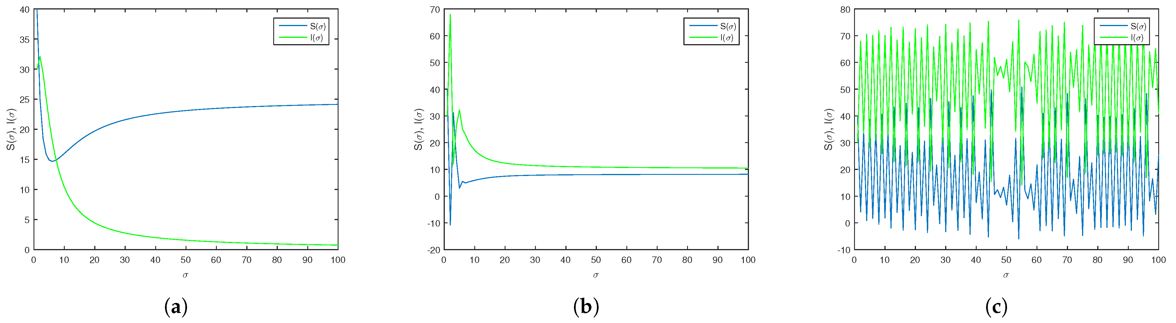
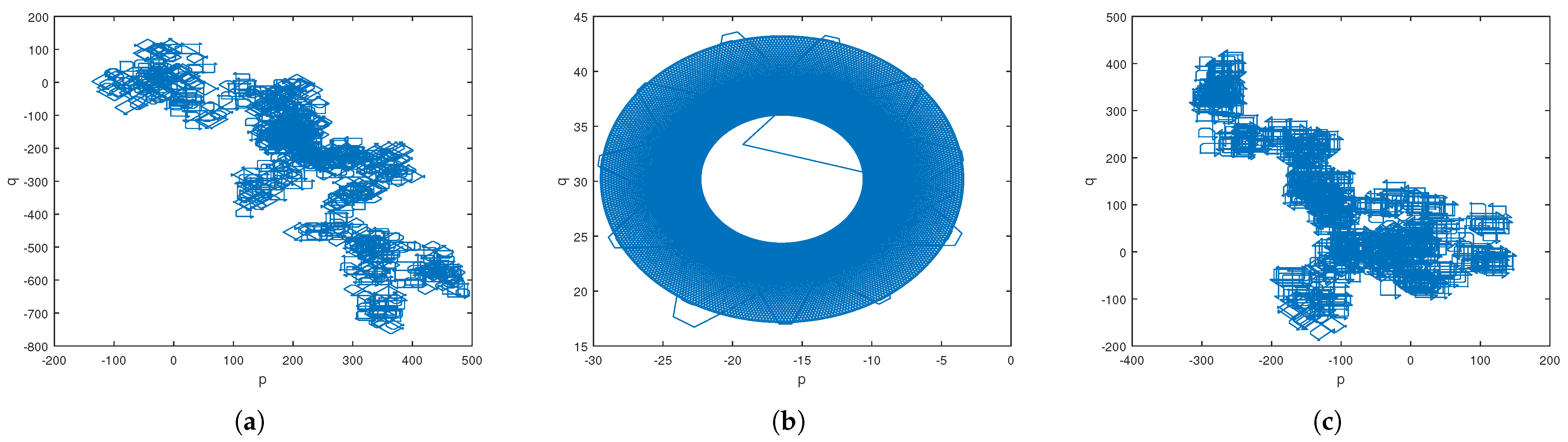
Example 1.

Consider System (12) with parameters $(b,\lambda ,d,ϵ)=(5,0.01,0.2,0.13)$ and $\eta =0.9$, which implies that $R_0=0.75<1$. Figure 1a demonstrates the stability of $E_0=(25,0)$.

Example 2.

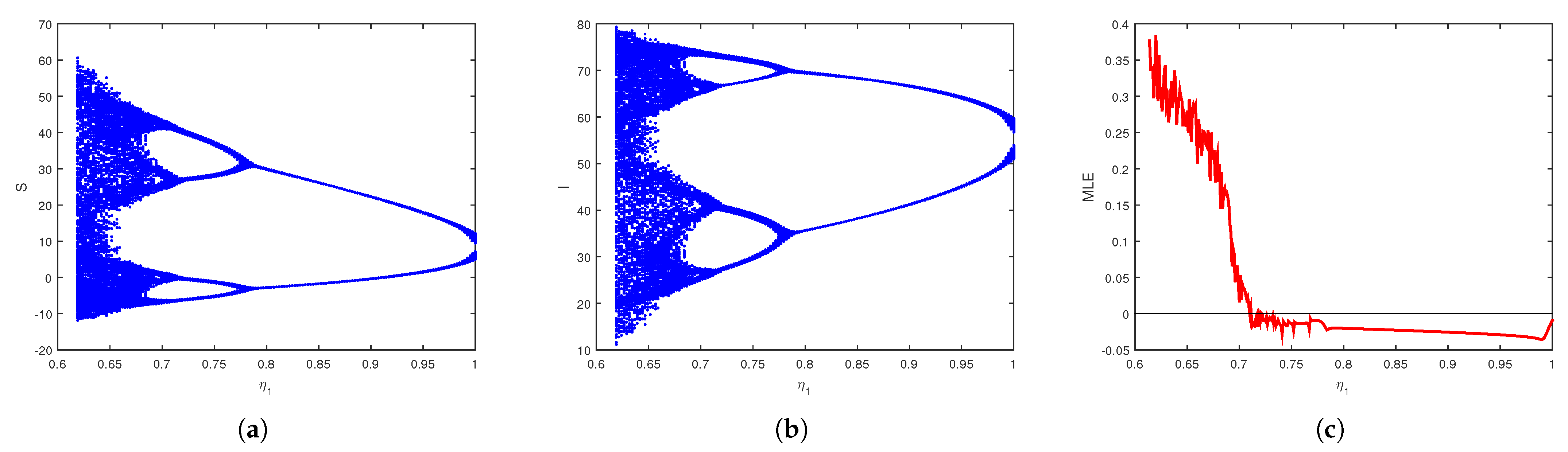
Let System (12) with parameters $(b,\lambda ,d,ϵ)=(5,0.04,0.2,0.13)$ and $\eta =0.9$, which implies that $R_0=3.03>1$. In Figure 1b, $E_{*}=(8.25,10.15)$ is confirmed to be stable.

Example 3.

Consider System (12) with parameters $(b,\lambda ,d,ϵ)=(20,0.04,0.2,0.13)$ and $\eta =0.4$, which implies that $R_0=12.1212$. Figure 1c highlights the chaotic dynamics of the system characterized by irregular and unpredictable fluctuations in its states. This behavior is typical of systems with sensitive parameters and fractional order variations, where small changes can lead to significantly different outcomes.

3.2. The Incommensurate Case

The focus of this section is the discrete computer virus model with incommensurate fractional orders. In such systems, each equation is governed by a distinct fractional order. The model is represented as follows:

$$\left\{\begin{array}{c}{}^c\Delta _{\rho }^{{\eta }_1}S\left(\sigma \right)=b-\lambda S(\sigma +{\eta }_1-1)I(\sigma +{\eta }_1-1)-dS(\sigma +{\eta }_1-1),\hfill \\ {}^c\Delta _{\rho }^{{\eta }_2}I\left(\sigma \right)=\lambda S(\sigma +{\eta }_2-1)I(\sigma +{\eta }_2-1)-ϵI(\sigma +{\eta }_2-1)-dI(\sigma +{\eta }_2-1).\hfill \end{array}\right.$$

(36)

Theorem 1 yields the following numerical model for system (36):

$$\left\{\begin{array}{c}S\left(\sigma \right)=S\left(0\right)+{\displaystyle \frac{1}{\mathrm{\Gamma }\left({\eta }_1\right)}}\sum _{j=1}^{\sigma }{\displaystyle \frac{\mathrm{\Gamma }(\sigma -j+{\eta }_1)}{\mathrm{\Gamma }(\sigma -j+1)}}[b-\lambda S(j-1)I(j-1)-dS(j-1)],\hfill \\ I\left(\sigma \right)=I\left(0\right)+{\displaystyle \frac{1}{\mathrm{\Gamma }\left({\eta }_2\right)}}\sum _{j=1}^{\sigma }{\displaystyle \frac{\mathrm{\Gamma }(\sigma -j+{\eta }_2)}{\mathrm{\Gamma }(\sigma -j+1)}}[\lambda S(j-1)I(j-1)-ϵI(j-1)-dI(j-1)].\end{array}\right.$$

(37)

Here, the stability properties of the discrete computer virus model with incommensurate orders are explored. The theorem presented below serves as a basis for investigating the stability of discrete fractional nonlinear models with incommensurate orders.

Theorem 3

([33]). For the following system where $0<{\eta }_{\iota }<1$ for $\iota =1,2,\dots ,n$.

$$\left\{\begin{array}{c}{}^c\Delta _0^{{\eta }_1}{\chi }_1\left(\sigma \right)={{\rm Y}}_1\left(\chi (\sigma +{\eta }_1-1)\right),\hfill \\ {}^c\Delta _0^{{\eta }_2}{\chi }_2\left(\sigma \right)={{\rm Y}}_2\left(\chi (\sigma +{\eta }_2-1)\right),\hfill \\ ⋮\hfill \\ {}^c\Delta _0^{{\eta }_n}{\chi }_n\left(\sigma \right)={{\rm Y}}_n\left(\chi (\sigma +{\eta }_n-1)\right),\hfill \end{array}\right.$$

(38)

where ${\rm Y}=({{\rm Y}}_1,{{\rm Y}}_2,\dots ,{{\rm Y}}_n):{\mathbb{R}}^n\to {\mathbb{R}}^n$ and $\chi \left(\sigma \right)={({\chi }_1\left(\sigma \right),{\chi }_2\left(\sigma \right),\dots ,{\chi }_n\left(\sigma \right))}^T\in {\mathbb{R}}^n$. M is the LCM of the denominators ${\varsigma }_{\iota }$ of ${\eta }_{\iota }$, where ${\eta }_{\iota }={\displaystyle \frac{{ϵ}_{\iota }}{{\varsigma }_{\iota }}}$, $({ϵ}_{\iota },{\varsigma }_{\iota })=1$ and ${ϵ}_{\iota },{\varsigma }_{\iota }\in {\mathbb{Z}}_{+}$ for $\iota =1,2,\dots ,n$. Put $i={\displaystyle \frac{1}{M}}$.

$$det\left(\mathit{diag}({\gamma }^{M{\eta }_1},{\gamma }^{M{\eta }_2},\dots ,{\gamma }^{M{\eta }_n})-(1-{\gamma }^M)\mathcal{J}\right)=0,$$

(39)

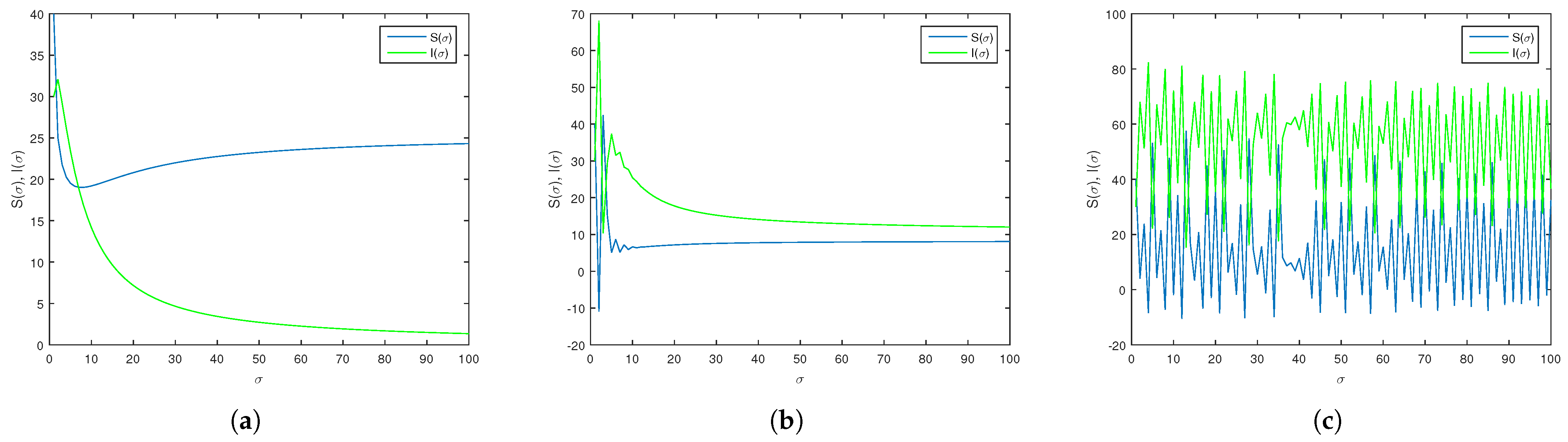
such that $\mathcal{J}$ is the Jacobian matrix of (38). If all eigenvalues of Equation (39) remain within $\mathbb{C}\backslash {Ł}^i$, Then, system (38) has a locally asymptotically stable trivial solution, such that

$${Ł}^i=\left\{l\in \mathbb{C}:\left|l\right|\le {\left(2cos{\displaystyle \frac{|arg(l\left)\right|}{i}}\right)}^i,\mathit{and}|arg\left(l\right)|\le {\displaystyle \frac{i\pi }{2}}\right\},$$

(40)

Example 4.

Consider system (36) with parameters $(b,\lambda ,d,ϵ)=(5,0.01,0.2,0.13)$, it follows that

$${\mathcal{J}}_0=\left(\begin{array}{cc}-0.2& -0.25\\ 0& -0.75\end{array}\right),$$

(41)

Let $({\eta }_1,{\eta }_2)=(0.68,0.86)$, which implies that $M=50$,

$$det\left(\left(\begin{array}{cc}{\gamma }^{34}& 0\\ 0& {\gamma }^{43}\end{array}\right)-(1-{\gamma }^{50}){\mathcal{J}}_0\right)=0,$$

(42)

equivalent to

$${\displaystyle \frac{1}{20}}(-{\gamma }^{50}+5{\gamma }^{34}+1)(-3{\gamma }^{50}+4{\gamma }^{43}+3)=0.$$

(43)

Solving Equation (43) yields 100 solutions, ${\gamma }_j(j=1,\dots ,100)$. All solutions remain within $\mathbb{C}\backslash {Ł}^{{\displaystyle \frac{1}{50}}}$. Theorem 3 proves the local asymptotic stability of $E_0$.

Example 5.

Consider System (36) with parameters $(b,\lambda ,d,ϵ)=(5,0.04,0.2,0.13)$, it follows that

$${\mathcal{J}}^{*}=\left(\begin{array}{cc}-0.606& -0.33\\ 0.406& 0\end{array}\right),$$

(44)

Let $({\eta }_1,{\eta }_2)=(0.68,0.86)$, which implies that $M=50$,

$$det\left(\left(\begin{array}{cc}{\gamma }^{34}& 0\\ 0& {\gamma }^{43}\end{array}\right)-(1-{\gamma }^{50}){\mathcal{J}}^{*}\right)=0,$$

(45)

equivalent to

$${\displaystyle \frac{6699}{50000}}{\gamma }^{100}-{\displaystyle \frac{303}{500}}{\gamma }^{93}+{\gamma }^{77}-{\displaystyle \frac{6699}{25000}}{\gamma }^{50}+{\displaystyle \frac{303}{500}}{\gamma }^{43}+{\displaystyle \frac{6699}{50000}}=0.$$

(46)

Solving Equation (46) yields 100 solutions, ${\gamma }_j(j=1,\dots ,100)$. All solutions remain in $\mathbb{C}\backslash {Ł}^{{\displaystyle \frac{1}{50}}}$. Theorem 3 demonstrates the local asymptotic stability of $E_{*}$.

Example 6.

Consider System (36) with parameters $(b,\lambda ,d,ϵ)=(20,0.04,0.2,0.13)$, it follows that

$${\mathcal{J}}_0=\left(\begin{array}{cc}-0.2& -4\\ 0& 3.67\end{array}\right),$$

(47)

Let $({\eta }_1,{\eta }_2)=(0.68,0.86)$, which implies that $M=50$,

$$det\left(\left(\begin{array}{cc}{\gamma }^{34}& 0\\ 0& {\gamma }^{43}\end{array}\right)-(1-{\gamma }^{50}){\mathcal{J}}_0\right)=0,$$

(48)

equivalent to

$${\displaystyle \frac{1}{500}}(-{\gamma }^{50}+5{\gamma }^{34}+1)(367{\gamma }^{50}+100{\gamma }^{43}-367)=0.$$

(49)

Solving Equation (49) yields 100 solutions, ${\gamma }_j(j=1,\dots ,100)$. Specifically, ${\gamma }_1=0.99504\in {Ł}^{{\displaystyle \frac{1}{50}}}$, satisfying $|{\gamma }_1|\le {\left(2cos\left(50\right|arg\left({\gamma }_1\right)\left|\right)\right)}^{{\displaystyle \frac{1}{50}}},\mathit{and}|arg\left({\gamma }_1\right)|\le {\displaystyle \frac{\pi }{100}}$. Theorem 3 provides a sufficient condition for the instability of $E_0$. And we have

$${\mathcal{J}}_{*}=\left(\begin{array}{cc}-2.4242& -0.33\\ 2.22424& 0\end{array}\right),$$

(50)

thus,

$$det\left(\left(\begin{array}{cc}{\gamma }^{34}& 0\\ 0& {\gamma }^{43}\end{array}\right)-(1-{\gamma }^{50}){\mathcal{J}}_{*}\right)=0,$$

(51)

equivalent to

$${\displaystyle \frac{917499}{1250000}}{\gamma }^{100}-{\displaystyle \frac{12121}{5000}}{\gamma }^{93}+{\gamma }^{77}-{\displaystyle \frac{917499}{625000}}{\gamma }^{50}+{\displaystyle \frac{12121}{5000}}{\gamma }^{43}+{\displaystyle \frac{917499}{1250000}}=0.$$

(52)

Solving Equation (52) yields 100 solutions, ${\gamma }_j(j=1,\dots ,100)$. There’s ${\gamma }_1=1.010355\in {Ł}^{{\displaystyle \frac{1}{50}}}$, satisfying $|{\gamma }_1|\le {\left(2cos\left(50\right|arg\left({\gamma }_1\right)\left|\right)\right)}^{{\displaystyle \frac{1}{50}}},\mathit{and}|arg\left({\gamma }_1\right)|\le {\displaystyle \frac{\pi }{100}}$. By Theorem 3, $E_0$ is unstable.

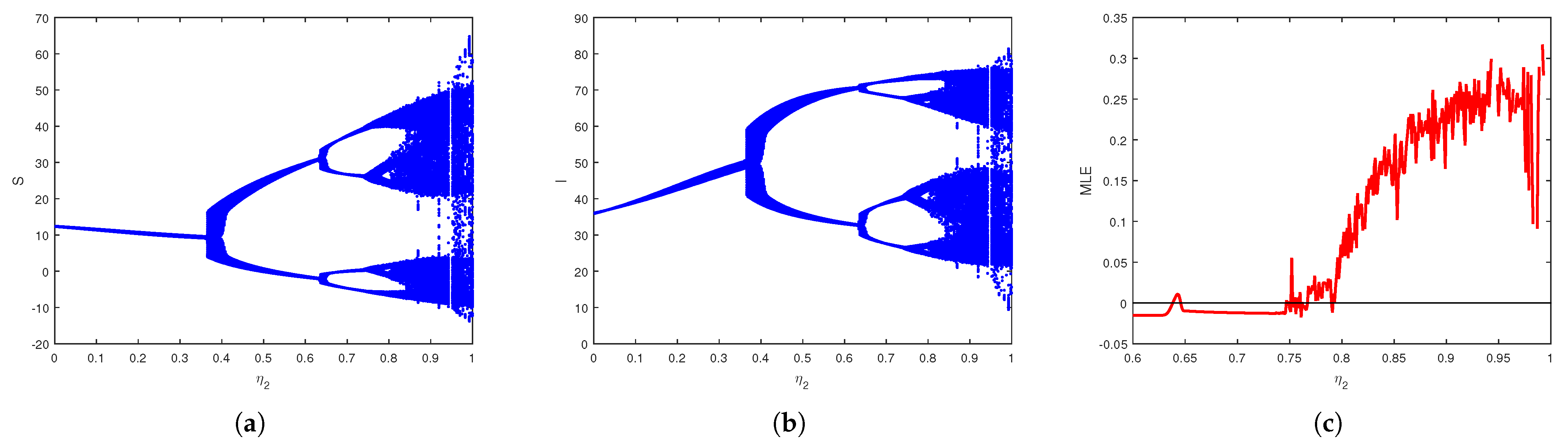
Based on the above, the computer virus incommensurate Model (36) is shown to satisfy a requirement for a chaotic attractor. Figure 2 shows the state evolution for the incommensurate Model (36) of the three previous examples with $({\eta }_1,{\eta }_2)=(0.68,0.86)$. In the following section, advanced analytical and numerical tools, such as Lyapunov exponents, bifurcation analysis, or phase space reconstruction, are necessary to fully understand and characterize its dynamics.

4. Dynamical Analysis and Simulation Results

The dynamics of System (12) will be characterized using numerical simulations, focusing on phase space representations, bifurcation diagrams, and the principal Lyapunov exponent (MLE) calculations, with the latter being determined via the Jacobian matrix algorithm [34]. A positive MLE indicates sensitive dependence on initial conditions, which signifies chaos. By definition, the Lyapunov exponent is

$$L{E}_{\iota }=\underset{\sigma \to \infty }{lim}{\displaystyle \frac{1}{\sigma }}ln\left|{\lambda }_{\iota }^{\left(\sigma \right)}\right|,for\iota =1,2,3.$$

(53)

where ${\lambda }_{\iota }$ ($\iota =1,2,3$) are the tangent map’s eigenvalues $J_{\sigma }$.

$$J_{\sigma }=\left(\begin{array}{cc}{f}_1\left(\sigma \right)& f_2\left(\sigma \right)\\ k_1\left(\sigma \right)& k_2\left(\sigma \right)\end{array}\right),$$

(54)

such that

$$\left\{\begin{array}{c}{f}_{\iota }\left(\sigma \right)=f_{\iota }\left(0\right)+{\displaystyle \frac{1}{\mathrm{\Gamma }\left(\eta \right)}}\sum _{j=1}^{\sigma }{\displaystyle \frac{\mathrm{\Gamma }(\sigma -j+\eta )}{\mathrm{\Gamma }(\sigma -j+1)}}((-\lambda I(j-1)-d)f_{\iota }(j-1)-\lambda S(j-1)k_{\iota }(j-1)),\hfill \\ k_{\iota }\left(\sigma \right)=k_{\iota }\left(0\right)+{\displaystyle \frac{1}{\mathrm{\Gamma }\left(\eta \right)}}\sum _{j=1}^{\sigma }{\displaystyle \frac{\mathrm{\Gamma }(\sigma -j+\eta )}{\mathrm{\Gamma }(\sigma -j+1)}}(\lambda I(j-1)f_{\iota }(j-1)+(\lambda S(j-1)-ϵ-d)k_{\iota }(j-1)),\end{array}\right.$$

(55)

using the identity matrix as initial conditions

$$\left(\begin{array}{cc}{f}_1\left(0\right)& f_2\left(0\right)\\ k_1\left(0\right)& k_2\left(0\right)\end{array}\right)=\left(\begin{array}{cc}1& 0\\ 0& 1\end{array}\right).$$

(56)

4.1. Commensurate Order Case

An investigation is conducted into the dynamic behavior variations of the proposed system (12) by constructing bifurcation diagrams; this approach allows visualization of the system’s long-term behavior as the parameter changes. Initially, the state is $\left(S\right(0),I(0\left)\right)=(40,30)$, the parameters used in the simulations are $(b,\lambda ,d,ϵ)=(20,0.04,0.2,0.13)$, and the commensurate order, denoted by $\eta$, is treated as the main bifurcation and sensitivity value due to its intrinsic role in governing the system’s memory and long-range interaction effects. By varying $\eta$ while keeping other model parameters constant, we were able to observe rich dynamical behaviors, including transitions from steady-state to periodic and chaotic regimes. This sensitivity to $\eta$ highlights its fundamental influence on the system’s stability and complexity. The resulting bifurcation diagram and the corresponding MLEs are seen in Figure 2. The bifurcation charts in Figure 3a,b depict system behavior for varying $\eta$ inside the interval $[0,1]$. These diagrams showcase various dynamical regimes, including stable fixed points, periodic oscillations, and chaotic dynamics. For small values of $\eta$ (approximately $\eta <0.2$), the system shows stable behavior, marked by a single fixed point or periodic oscillations. As $\eta$ increases beyond this range, a series of period-doubling bifurcations occurs, leading to the emergence of chaos around $\eta =0.25$. The chaotic regime is evident in the bifurcation diagrams, where the state variable displays an irregular and dense structure, reflecting initial condition sensitivity. This chaotic behavior persists roughly in the range $0.25\le \eta \le 0.7$, during which the system exhibits complex, non-periodic oscillations. The transition from order to chaos is further supported by the MLEs plot in Figure 2c. For $\eta <0.2$, the MLE remains negative, confirming stability. As $\eta$ approaches $0.25$, the MLE crosses zero and becomes positive, signaling the onset of chaos. The chaotic regime is most pronounced in the interval $0.25\le \eta \le 0.7$, where the MLE remains significantly positive, peaking around $\eta =0.5$. This indicates a high degree of unpredictability and sensitivity to initial conditions. Beyond $\eta =0.7$, the system gradually transitions back to stability, as indicated by decreasing MLE values. For $\eta >0.8$, the MLE becomes negative again, suggesting a return to periodic or fixed-point behavior. This demonstrates that while moderate values of $\eta$ induce chaotic dynamics, higher values restore stability.

The commensurate fractional discrete computer virus System (12) exhibits a range of dynamical behaviors, as illustrated by the phase portraits in Figure 4. For different values of $\eta$, the figure shows chaos at lower fractional orders $\eta$ values. The choice of fractional orders in our simulations was guided by the goal of exploring transitions in system dynamics. Specific values were selected to capture the onset of chaotic behavior, as verified by positive Lyapunov exponents. These numerical simulations highlight the system’s interesting dynamical properties. The oscillatory nature is due to nonlinearity and fractional memory, especially when chaos emerges. Fractional-order systems are known to exhibit oscillations even in the absence of external forcing.

In summary, these findings emphasize the significant contribution of the fractional derivative parameter $\eta$ in shaping the system’s complexity. The occurrence of bifurcations and chaos within specific intervals highlights the rich dynamical behavior of fractional-order models, making them particularly valuable for studying complex systems. The capacity of fractional-order models to effectively simulate the delayed propagation and reinfection cycles characteristic of known computer worms, such as WannaCry or Conficker, positions them as a suitable tool for cyber-epidemiological forecasting. This ability underscores the significant role of fractional calculus in providing deeper insights into the intricate dynamics of digital epidemics. By offering a more nuanced understanding of virus transmission patterns, these models can ultimately aid in the development of more advanced and effective cybersecurity strategies.

4.2. Incommensurate Order Case

Combined analysis of the bifurcation diagrams (Figure 5a,b) and the largest Lyapunov exponent plot (Figure 5c) reveals the complex dynamics of the incommensurate System (36) as the fractional order parameter ${\eta }_1$ is varied, with ${\eta }_2$ fixed at $0.86$. For small values of ${\eta }_1$ in the range $[0.25,0.55]$, the system displays chaos, as indicated by the dense and irregular patterns in the bifurcation diagrams. This chaotic regime is further confirmed by the MLE plot, where the exponent remains positive, signifying sensitive dependence on initial conditions. As ${\eta }_1$ increases beyond approximately $0.55$, the system transitions from chaos to periodic behavior through a period-doubling route, with distinct branches emerging in the bifurcation diagrams. This transition is also evident in the MLE plot Figure 5c, where the exponent gradually decreases and becomes negative around ${\eta }_1=0.7$, indicating the system’s stabilization. For ${\eta }_1>0.7$, the system enters a periodic or steady-state regime, characterized by well-defined trajectories.

Figure 6 provides a comprehensive view of the dynamic behavior of an incommensurate system as the fractional order ${\eta }_2$ is varied, while ${\eta }_1$ is held constant at $0.68$. The bifurcation diagrams in Figure 6a,b depict the system’s response to changes in ${\eta }_2$, showcasing a rich tapestry of periodic windows interspersed with chaotic regions. This intricate pattern suggests a high sensitivity to variations in ${\eta }_2$, implying that even small changes in this parameter can significantly alter the system’s long-term behavior. Further evidence of this sensitivity is provided by the Maximum Lyapunov Exponent plot in Figure 6c. The MLE, a crucial indicator of chaoticity, fluctuates between positive and negative values. Positive MLE values signify chaotic behavior, marked by sensitivity to initial conditions, while negative values indicate periodic or stable behavior. The observed fluctuations in the MLE confirm the system’s tendency to transition between these distinct dynamical regimes as ${\eta }_2$ is adjusted. This dynamic interplay between order and chaos underscores the complex nature of the system and its intricate response to parameter variations. In essence, Figure 6 reveals a system with a delicate balance between order and chaos, while Figure 7 shows various phase portraits for different incommensurate orders. The bifurcation diagrams and the MLE plot collectively demonstrate that the system’s behavior is remarkably sensitive to fractional order ${\eta }_2$ changes. These findings highlight the significant role of the fractional parameter in governing the system’s stability and complexity. Understanding the transition between chaotic and periodic behavior provides critical insights into computer virus propagation dynamics, aiding in the development of more effective cybersecurity strategies and mitigation techniques. In contrast, statistical-fitting approaches (e.g., [35]), while accurate in reproducing specific outbreak curves, do not capture the memory-dependent and chaotic behavior observed in real-world propagation scenarios. The model adds dynamic interpretability and flexibility through its fractional-order structure, allowing it to simulate a wider range of propagation patterns through parameter tuning.

4.3. Simulation Results

To rigorously address concerns regarding the real-world applicability of our fractional-order model to computer virus propagation (12), we introduce a comprehensive case study focusing on the Stuxnet worm. This prominent real-world virus targeted industrial control systems, with its 2010 outbreak in Iran serving as a critical dataset for model validation. The empirical data describing Stuxnet’s spread were obtained from Masood et al. [36], and we carefully calibrated the parameters of our fractional model to align with this time series.

Table 1. Model parameters for various simulation cases.

Parameters	Case 1	Case 2	Case 3	Case 4
b	0.042	40	100	5600
$\lambda$	0.385	0.385	0.4	0.4
d	0.1126	0.0804	0.1598	0.1276
$ϵ$	0.11525	0.0814	0.16	0.021

and

Table 2. Initial values of variables used in the simulation of different scenarios.

Variables	S	I
Case 1	$2.3\times {10}^6$	10,000
Case 2–4	$2.3\times {10}^6$	30,000

present the parameter values and initial conditions used in the simulations, respectively.

The numerical simulations were performed using a step size of $h={10}^{-6}$ to ensure high accuracy in approximating the fractional-order differences. As shown in Figure 8, the simulation results generated by our model exhibit strong agreement with the actual diffusion trajectory of Stuxnet. The model accurately captures the early exponential growth, the inflection point, and the eventual saturation behavior hallmarks of real-world virus propagation. This close correspondence between simulation and observation confirms that the proposed fractional-order model effectively represents the dynamics of real computer virus outbreaks, thereby reinforcing its practical relevance and directly addressing the reviewer’s concerns.

The numerical simulation of the discrete fractional-order SI model is based on the Caputo-like difference operator. The algorithm follows a step-by-step iterative scheme to compute the values of $S\left(\sigma \right)$ and $I\left(\sigma \right)$ over time. The procedure can be summarized as follows:

• Set the initial conditions $S\left(0\right)$, $I\left(0\right)$, and parameters $(b,\lambda ,d,ϵ)$.
• Set the fractional order $\eta$ and total simulation steps N.
• For each time step $\sigma =0$ to N:
  • Compute the fractional sums according to the Caputo-like formula:

    $${}^c\Delta _{\rho }^{\eta }f\left(\sigma \right)={\Delta }_{\rho }^{-(\delta -\eta )}{\Delta }^{\delta }f\left(\sigma \right)$$
  • Update $S(\sigma +1)$ and $I(\sigma +1)$ using the model equations.
• Save or plot the values at each step for bifurcation, chaos, and entropy analyses.

The simulation flowchart is given in the next Figure 9.

5. Complexity Algorithms

The complexity of chaotic behavior is analyzed to evaluate chaotic systems.Using the spectral and approximate entropy algorithms, a complexity analysis is performed on the fractional discrete virus model, and the 0 − 1 test confirms the occurrence of chaos.

5.1. $0-1$ Test

To discern chaos from regularity behavior, the 0−1 test is applied, which was developed by Gottwald and Melbourne [37]. Inputting time series data, the test yields an output close to 1 for chaotic dynamics and close to 0 for regular behavior. The test is described below.

The first step is to use the time series $\phi \left(n\right)$ for $n=1,2,\dots ,N$ to define the translation variables in the following manner:

$$p_c\left(k\right)=\sum _{n=1}^k\phi \left(n\right)cos\left(ic\right);q_c\left(k\right)=\sum _{n=1}^k\phi \left(n\right)sin\left(ic\right);k=1,2,\dots ,N.$$

(57)

The fractional discrete computer virus model exhibits either regular or chaotic behavior, which is determined using the $(p_c-q_c)$ chart. Regular dynamics are associated with bounded trajectories of $p_c$ and $q_c$, while chaotic dynamics are characterized by Brownian-like motion. The mean square displacement formula, used in this analysis, is given by

$$M_c\left(k\right)={\displaystyle \frac{1}{N}}\sum _{n=1}^N\left[{(p_c(n+k)-p_c\left(n\right))}^2+{(q_c(n+k)-q_c\left(n\right))}^2\right],k\le {\displaystyle \frac{N}{10}}.$$

(58)

Asymptotic growth is represented in the final step as follows:

$$K_c=\underset{k\to \infty }{lim}{\displaystyle \frac{log{M}_c}{logk}}.$$

(59)

The growth rate $k=median\left(K_c\right)$ is vital in distinguishing the onset of chaotic motion from a nonchaotic state in the proposed model (12). Specifically, when the value of k is close to 0, it indicates that the model exhibits nonchaotic behavior. Conversely, as the value of k goes to 1, it indicates that the model’s dynamics are chaotic.

Both the commensurate (12) and incommensurate (36) order computer virus models are examined for chaotic behavior using $(p-q)$ plots. The results, shown in Figure 10 for the parameter values used $(b,\lambda ,d,ϵ)=(20,0.04,0.2,0.13)$, (a) with $\eta =0.4$, (b) with $\eta =0.9$, and (c) with the incommensurate derivatives ${\eta }_1=0.63$, ${\eta }_2=0.86$. It reveals a clear distinction between periodic behavior (bounded trajectories, Figure 10b) and chaotic motion (Brownian-like trajectories, Figure 10a,c).

5.2. Spectral Entropy Test

Spectral Entropy (SE) measures disorder in the frequency domain [38]. Higher SE values, corresponding to flatter power spectra, indicate greater time series complexity. SE is calculated as follows: For a discrete time series $\left\{x\right(\sigma ),\sigma =0,1,2,\dots ,N-1\}$ of length N, the mean-adjusted series is $x\left(\sigma \right)=x\left(\sigma \right)-\overline{x},$ where $\overline{x}$ is the mean. The Discrete Fourier Transform (DFT) is given by

$$\chi \left(k\right)=\sum _{\sigma =0}^{N-1}x\left(\sigma \right)e^{-2j\pi \sigma k/N},$$

(60)

where k takes values from 0 to $N-1$, and j is the imaginary unit. The frequency spectrum at frequency index k is given by ${\left|\chi \left(k\right)\right|}^2$, and the normalized probability distribution of the spectral power is defined as

$$P_k={\displaystyle \frac{{\left|\chi \left(k\right)\right|}^2}{{\sum }_{k=0}^{N/2-1}{\left|\chi \left(k\right)\right|}^2}},$$

(61)

Applying the DFT, corresponding to k values from 0 to $N/2-1$. The spectral entropy is then represented as

$$SE={\displaystyle \frac{{\sum }_{k=0}^{N/2-1}{P}_{k}ln\left(P_k\right)}{ln(N/2)}},$$

(62)

where $ln(N/2)$ represents random signal entropy.

Given the parameter values $(b,\lambda ,d,ϵ)=(20,0.01,0.2,0.8)$, the SE complexity analysis outcomes for the fractional System (12), across a range of derivative orders, are shown in Figure 11.

Fractional orders clearly influence system dynamics. Figure 11a demonstrates that the commensurate model (12) achieves a high complexity level when $\eta \in [0.18,0.45]$. Similarly, as shown in Figure 11b, for ${\eta }_2=0.86$, the complexity of (36) varies with ${\eta }_1$. Notably, when ${\eta }_1$ nears $0.62$, the system reaches its highest complexity. Additionally, in Figure 11c, the impact of ${\eta }_2$ can be observed on the dynamic behavior when ${\eta }_1=0.68$. It is evident that complexity increases as ${\eta }_2$ varies, reaching its peak when ${\eta }_2$ approaches 1. These observations align with the findings from the largest Lyapunov exponent. Thus, for complex real-world applications, choosing appropriate fractional orders is crucial.

5.3. Approximate Entropy Test

The complexity of the commensurate (12) and incommensurate (36) computer virus models is analyzed using Approximate Entropy (ApEn). ApEn is a method for quantifying disorder and unpredictability in time series; higher ApEn values indicate greater complexity and chaotic behavior, and its algorithm is described in reference [39] as

$$ApEn={{\rm Y}}^n\left(r\right)-{{\rm Y}}^{n+1}\left(r\right),$$

(63)

such as ${{\rm Y}}^n\left(r\right)$ is given by

$${{\rm Y}}^n\left(r\right)={\displaystyle \frac{1}{m-n+1}}\sum _{\iota =1}^{m-n+1}log{C}_{\iota }^n\left(r\right),$$

(64)

where $r=0.2std\left(\chi \right)$ and $m=2$, the standard deviation of the data $\chi$ is denoted by $std\left(\chi \right)$. Figure 12 presents the Approximate Entropy (ApEn) for both the commensurate (12) and incommensurate (36) models. The analysis was performed with $(b,\lambda ,d,ϵ)=(20,0.01,0.2,0.8)$. Specifically, the figure shows ApEn as a function of $\eta$ (Figure 12a), ${\eta }_1$ with ${\eta }_2$ fixed at $0.86$ (Figure 12b), and ${\eta }_2$ with ${\eta }_1$ fixed at $0.68$ (Figure 12c). The high ApEn values observed in both models demonstrate significant complexity, consistent with both the ApEn calculation itself and the observed system behavior. Furthermore, positive MLE values confirm the presence of chaos, while the ApEn values quantify the associated disorder and unpredictability. The MLE and ApEn analyses show a strong correlation in their characterization of the system’s dynamics. To demonstrate the added value of fractional-order modeling, we compare the dynamics of the proposed model with its classical integer-order counterpart. The fractional model exhibits richer and more complex dynamics, as evidenced by bifurcation behavior and entropy measures.

6. Conclusions and Future Directions

This study investigates the stability and chaotic dynamical behavior exhibited by a fractional discrete SI model designed for computer viruses, focusing on both commensurate and incommensurate fractional orders. By leveraging fractional calculus, long-term dependencies in virus transmission are captured, offering a more realistic depiction of digital epidemics. The stability analysis, based on the reproduction number $R_0$, delineates the conditions under which the virus spreads is either contained or persists.

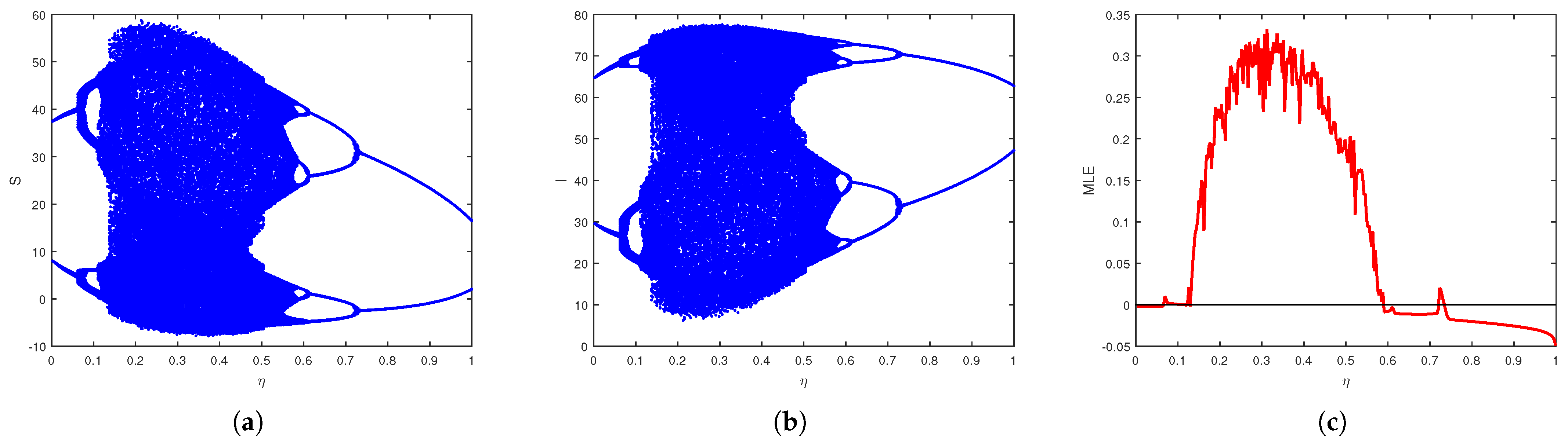
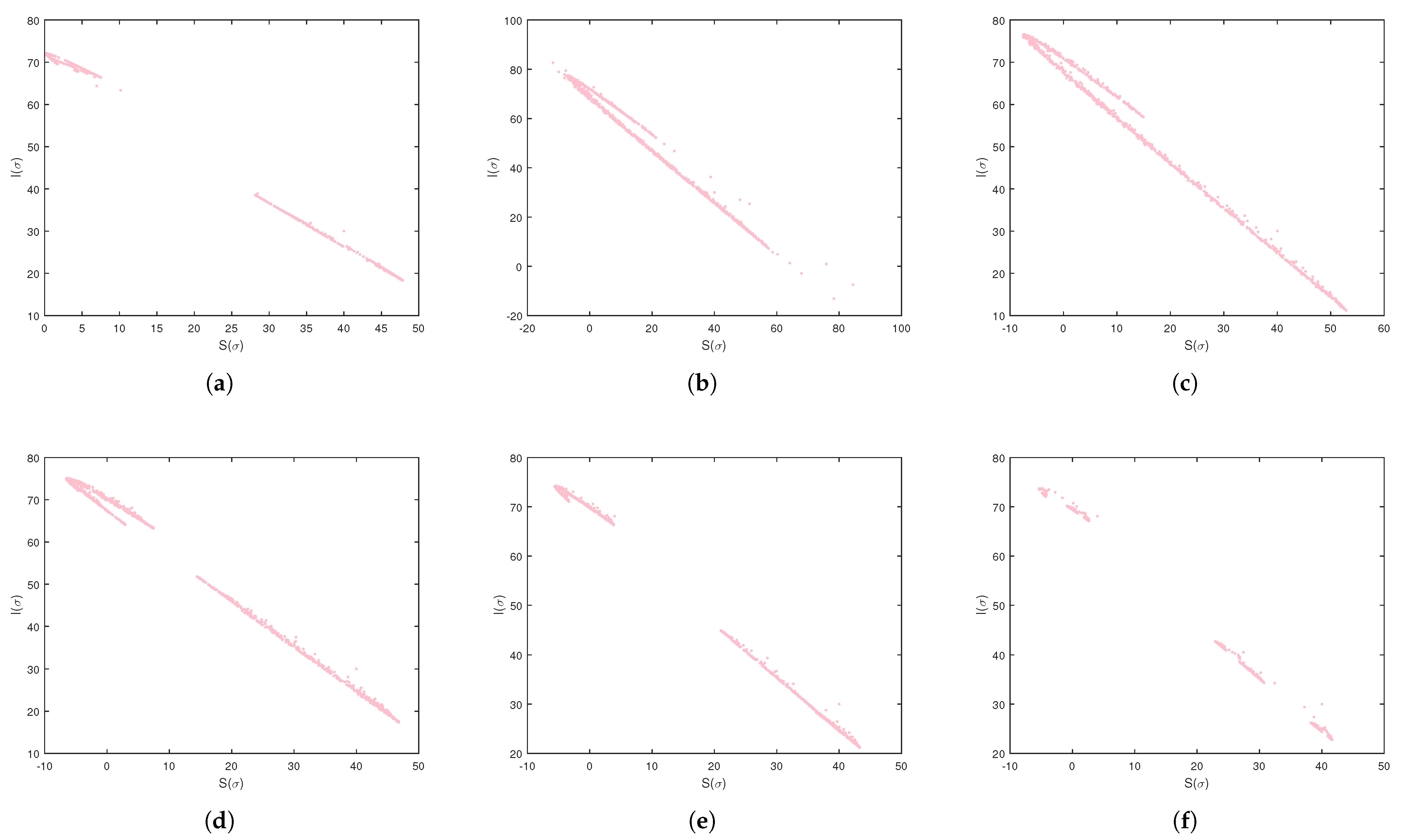
Moreover, numerical investigations reveal that the system exhibits chaotic behavior in certain parameter regimes, with commensurate and incommensurate fractional orders introducing more intricate and unpredictable dynamics. To systematically examine the chaotic nature of the model, multiple analytical techniques were employed, including bifurcation diagrams, phase portraits, and the maximum Lyapunov exponent. Sophisticated complexity algorithms confirmed the system’s nonlinear and chaotic nature, utilizing spectral entropy, approximate entropy, and the $0-1$ test. These tools provided a comprehensive characterization of the system’s nonlinear behavior, confirming that fractional order plays a crucial role in shaping the model’s dynamical properties. The findings indicate that fractional orders contribute to heightened complexity, emphasizing the need for advanced cybersecurity strategies to address unpredictable virus propagation.

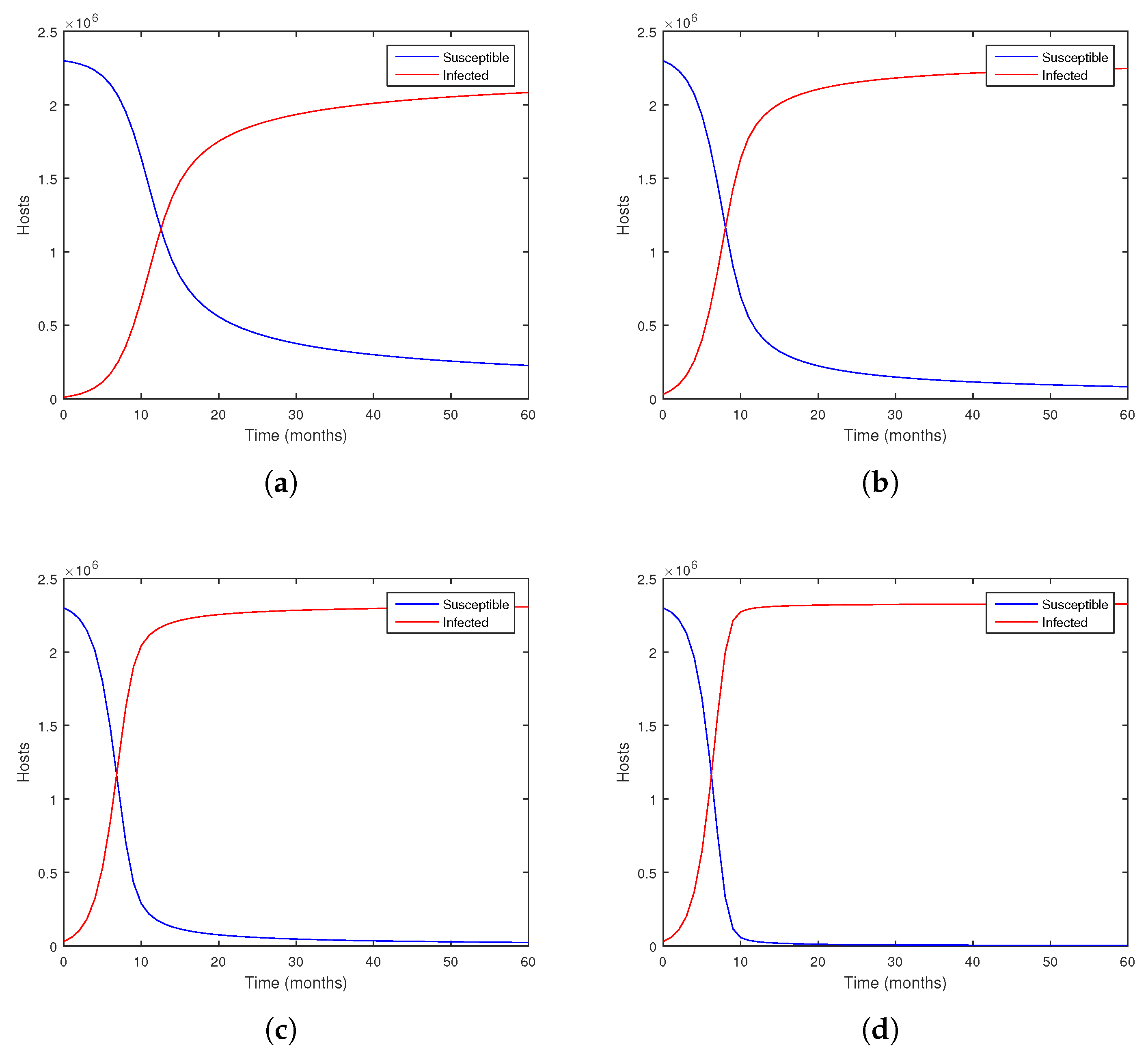
While the current study initially focused on theoretical development and numerical analysis, a critical step towards demonstrating its practical utility involved bridging the gap to real-world applicability by applying the model to the well-documented case of the Stuxnet worm. Using empirical time-series data from Masood et al. [36], the parameters were calibrated, and the fractional-order model was shown to accurately reproduce the virus’s diffusion trajectory. This real-world validation highlights the model’s practical potential.

Although retrospective modeling approaches, such as the one by Milošević [35], offer valuable statistical descriptions of cyberattacks, they often lack dynamic interpretability and flexibility. In contrast, the fractional-order framework proposed here offers a dynamic and tunable structure that can simulate complex virus behaviors, including chaos via memory effects and fractional parameters. Although tailored for computer virus propagation, the proposed model structure can be adapted to study biological epidemics by redefining the compartments and transition parameters, making it broadly applicable in epidemiological modeling.

In future work, this validation will be extended to other real cyber threats, such as Conficker or WannaCry, and the generalizability of the model across different virus types will be explored. Plans also include integrating optimization-based data-fitting techniques to refine parameter estimation and collaborating with cybersecurity professionals to evaluate the model’s integration into early detection systems, response mechanisms, and cryptographic schemes that leverage chaotic dynamics. By building on real-world data, the aim is to further enhance the impact of this model on both theoretical understanding and practical cybersecurity applications.