Article

Frost Resistance Prediction of Concrete Based on Dynamic Multi-Stage Optimisation Algorithm

1
Key Laboratory of Opto-Electronic Technology and Intelligent Control, Ministry of Education, Lanzhou Jiaotong University, Lanzhou 730070, China
2
National and Provincial Joint Engineering Laboratory of Road & Bridge Disaster Prevention and Control, Lanzhou Jiaotong University, Lanzhou 730070, China
3
School of Materials Science and Engineering, Southeast University, Nanjing 211189, China
*
Author to whom correspondence should be addressed.
Algorithms 2025, 18(7), 441; https://doi.org/10.3390/a18070441
Submission received: 18 June 2025 / Revised: 13 July 2025 / Accepted: 17 July 2025 / Published: 18 July 2025

Abstract

Concrete in cold areas is often subjected to a freeze–thaw cycle period, and a harsh environment will seriously damage the structure of concrete and shorten its life. The frost resistance of concrete is primarily evaluated by relative dynamic elastic modulus and mass loss rate. To predict the frost resistance of concrete more accurately, based on the four ensemble learning models of random forest (RF), adaptive boosting (AdaBoost), categorical boosting (CatBoost), and extreme gradient boosting (XGBoost), this paper optimises the ensemble learning models by using a dynamic multi-stage optimisation algorithm (DMSOA). These models are trained using 7090 datasets, which use nine features as input variables; relative dynamic elastic modulus (RDEM) and mass loss rate (MLR) as prediction indices; and six indices of the coefficient of determination (R2), mean square error (MSE), root mean square error (RMSE), mean absolute error (MAE), correlation coefficient (CC), and standard deviation ratio (SDR) are selected to evaluate the models. The results show that the DMSOA-CatBoost model exhibits the best prediction performance. The R2 of RDEM and MLR are 0.864 and 0.885, respectively, which are 6.40% and 11.15% higher than those of the original CatBoost model. Moreover, the model performs better in error control, with significantly lower MSE, RMSE, and MAE and stronger generalization ability. Additionally, compared with the two mainstream optimisation algorithms (SCA and AOA), DMSOA-CatBoost also has obvious advantages in prediction accuracy and stability. Related work in this paper has a certain significance for improving the durability and quality of concrete, which is conducive to predicting the performance of concrete in cold conditions faster and more accurately to optimise the concrete mix ratio whilst saving on engineering cost.

1. Introduction

Concrete is one of the most important building materials in the construction industry and is widely used in construction projects in different climatic environments [1]. Owing to the special geographical and climatic conditions, the freeze–thaw cycle caused by the long, dry, and cold climate and the large temperature difference between day and night will markedly shorten the life of concrete in cold plateau areas. In severe cases, it can cause damage or functional failure of concrete structures and even lead to serious casualties, economic losses, and extensive social impacts [2]. Thus, the frost resistance of concrete has become an important factor to ensure the safety and durability of buildings in these types of areas [3]. In cold environments, the relative dynamic elastic modulus and mass loss rate can effectively characterise the frost resistance of concrete [4]. These two evaluation indicators reflect the changes in physical and mechanical properties of concrete during freeze–thaw cycles, which are crucial for understanding and improving the frost resistance of concrete.
In recent years, many studies have examined the frost resistance of concrete. From the aspect of additives in concrete, Craeye et al. [5] used superabsorbent polymer instead of an air entrainer in concrete, which improved the freeze–thaw resistance of concrete road infrastructure. Bian et al. [6] found that adding basalt fibre can substantially improve the freeze–thaw resistance and sulphate attack resistance of concrete. Wang et al. [7] found that concrete with 2% nano-silica added can improve its frost resistance under the freeze–thaw cycle condition of −40 °C to + 5 °C. Liu et al. [8] used organic and inorganic crystalline materials to study the frost resistance of concrete by surface coating and soaking and found that organic crystalliser can increase the frost resistance by 2.5 times. He et al. [9] found that 15% microbead content can highly improve the strength and frost resistance of expanded polystyrene concrete. In addition, from the aspect of concrete structural characteristics, Liu et al. [10] found that the porosity, aggregate particle size, and water/binder ratio of porous concrete had significant effects on its frost resistance. Zhou et al. [11] found that the larger the particle size of aggregate, the greater the heterogeneity of the internal structure of concrete, which will lead to further defects and weaknesses and serious damage during freeze–thaw cycles. Du et al. [12] found that the pores of 3D-printed concrete primarily gathered near the interface; additionally, the porosity of the interlayer interface was lower than that of the interwire interface, thus showing excellent frost resistance. The traditional experimental methods used in the above research often require a long time and cost. Thus, with the rapid development of computer technology, ensemble learning algorithms have shown remarkable potential in solving complex problems in many engineering and scientific fields [13]. Some scholars have also used ensemble learning algorithms to study concrete performance prediction, especially frost resistance. Li et al. [14] established a prediction model of concrete freeze–thaw mass loss rate with high accuracy and strong generalisation ability based on support vector machine regression and random forest regression. Tang et al. [15] combined random forest and wavelet neural network technology, selected the influencing factors from the proportion of concrete materials, and established a high-precision prediction model of concrete frost resistance. Wang et al. [16] proposed an effective method for predicting the frost resistance of concrete by optimising the concrete ratio index by using a random forest algorithm. Gao et al. [17] established six ML models, and the performance statistics show that the XGBoost ensemble learning algorithm based on boosting has the best prediction performance for the frost resistance of rubber concrete. However, the existing study based on ensemble learning models such as RF and SVM still has some drawbacks. These models are prone to errors when dealing with imbalanced sample distributions and strong nonlinear correlations among variables. Moreover, the performance of these models is highly sensitive to the setting of hyperparameters, which requires manual adjustment based on experience and thus cannot guarantee optimal performance in multi-feature complex datasets. Meanwhile, such methods often lack a global search mechanism, making them prone to getting stuck in local optima, resulting in poor stability of the prediction results and limited generalization ability. The application of an intelligent optimisation algorithm can somewhat overcome these problems. Zhang et al. [18] adopted the Bayesian optimisation random forest ensemble learning method to establish a three-stage frost resistance prediction model for an accurate and quick prediction of the frost resistance of concrete. Chen et al. [19] proposed the use of NSGA-II in optimising the random forest model to improve the frost resistance of concrete in severe cold areas, realise the economic and environmentally friendly production of concrete, and improve the safety performance and service life of the project.
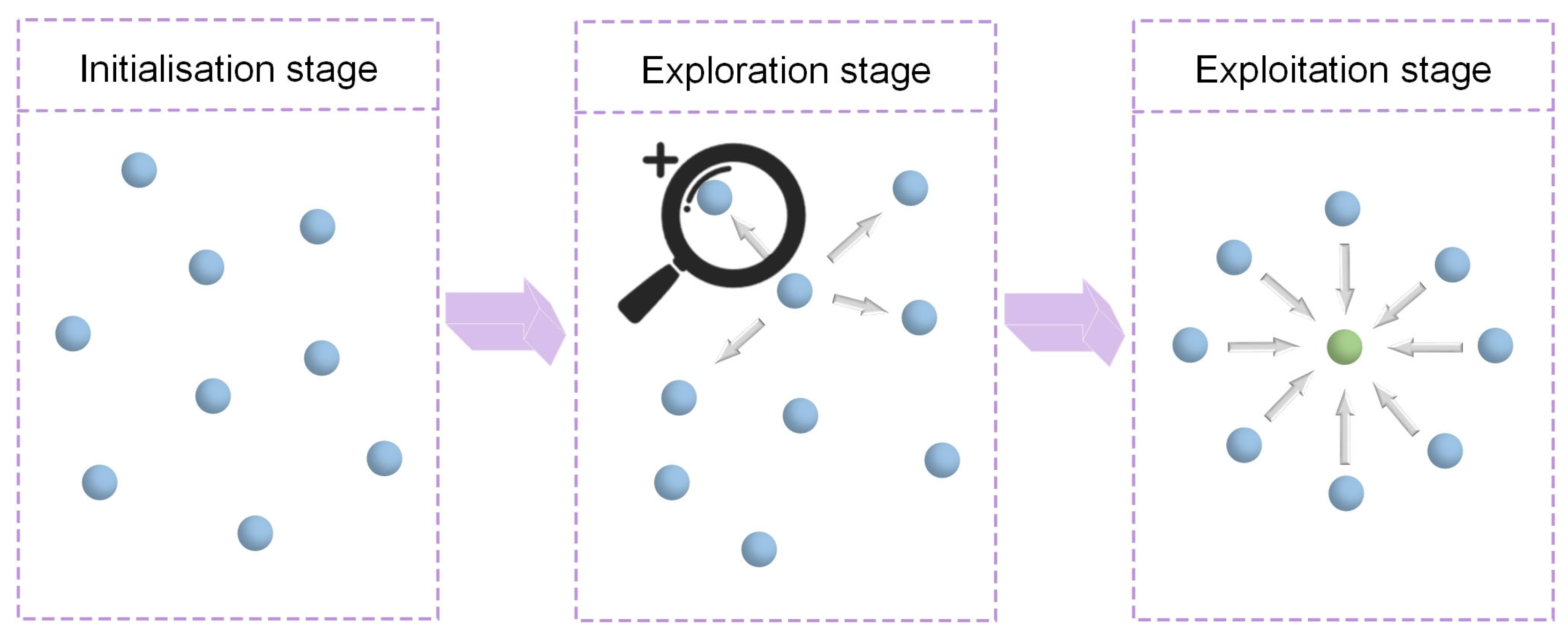
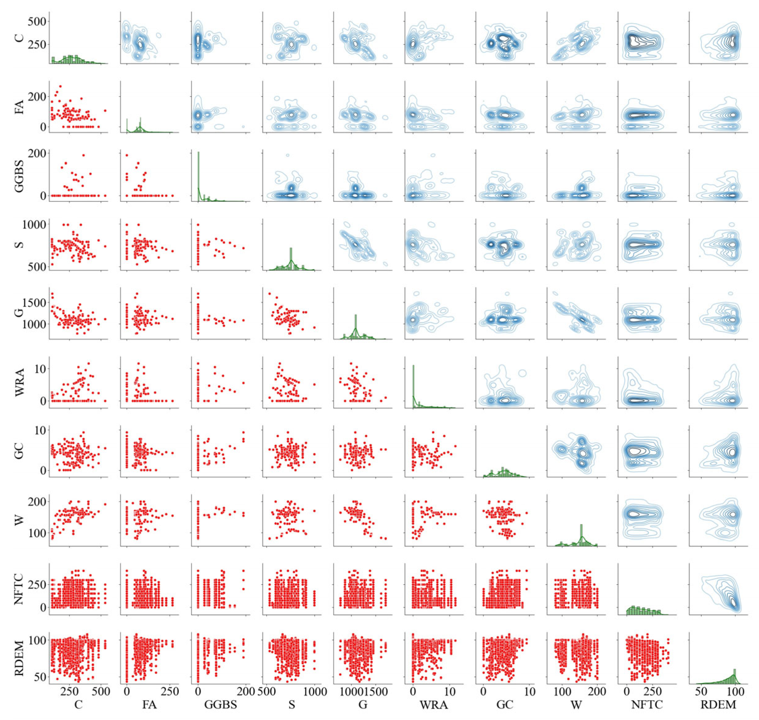
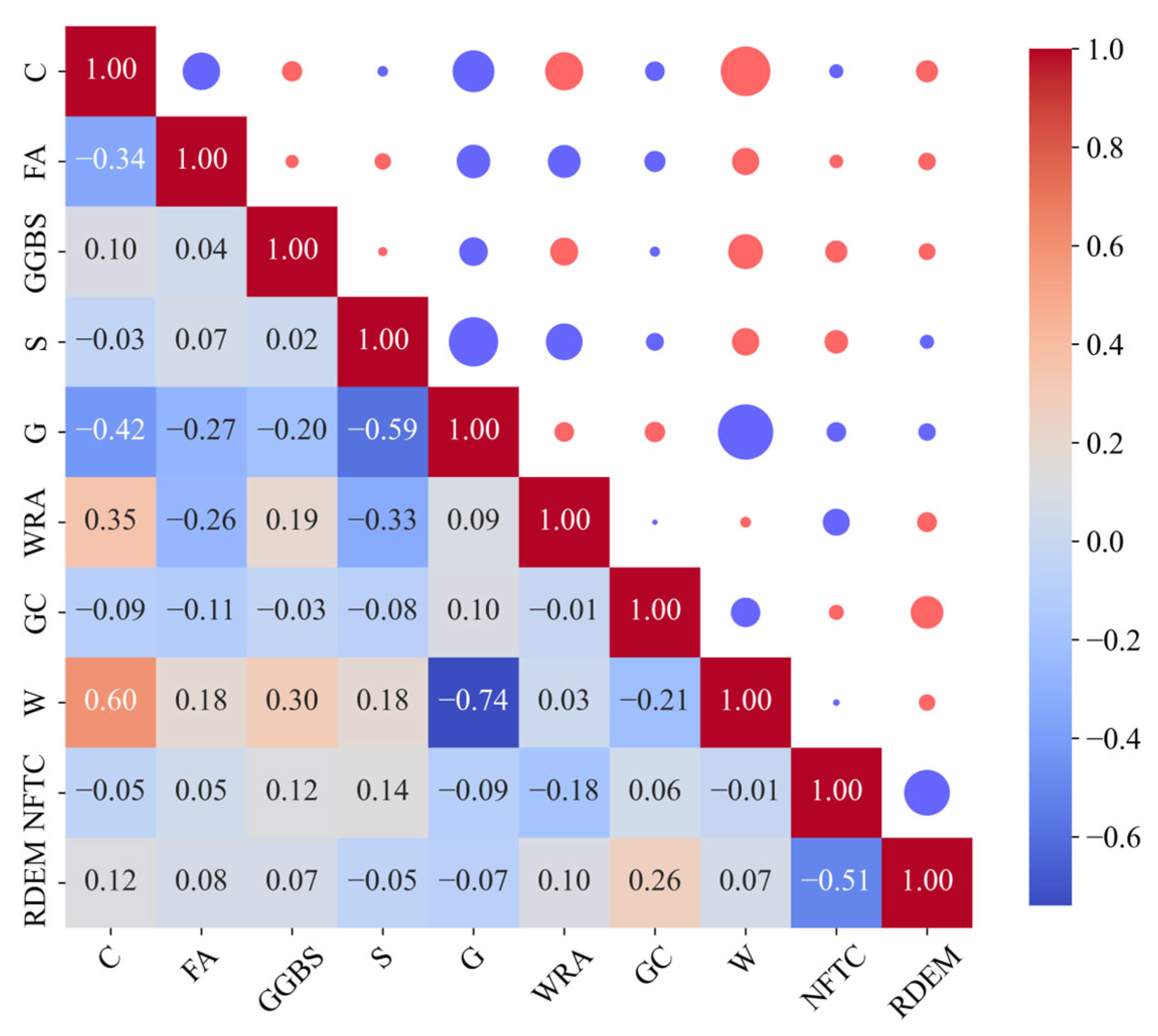
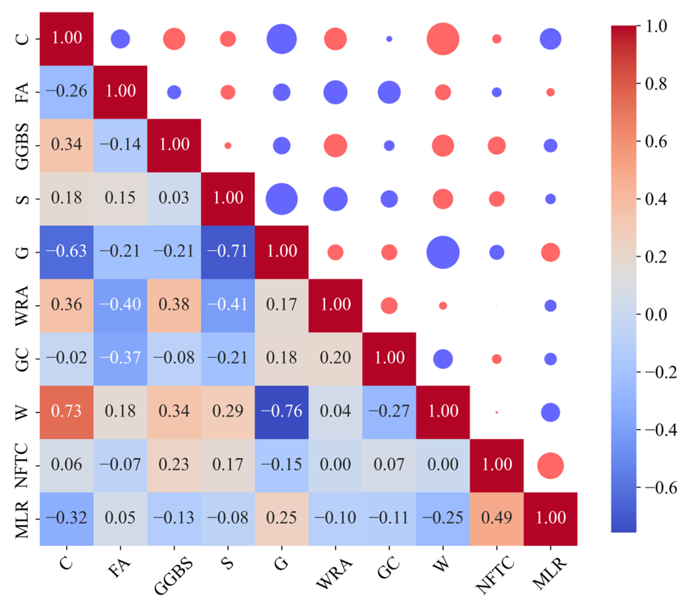
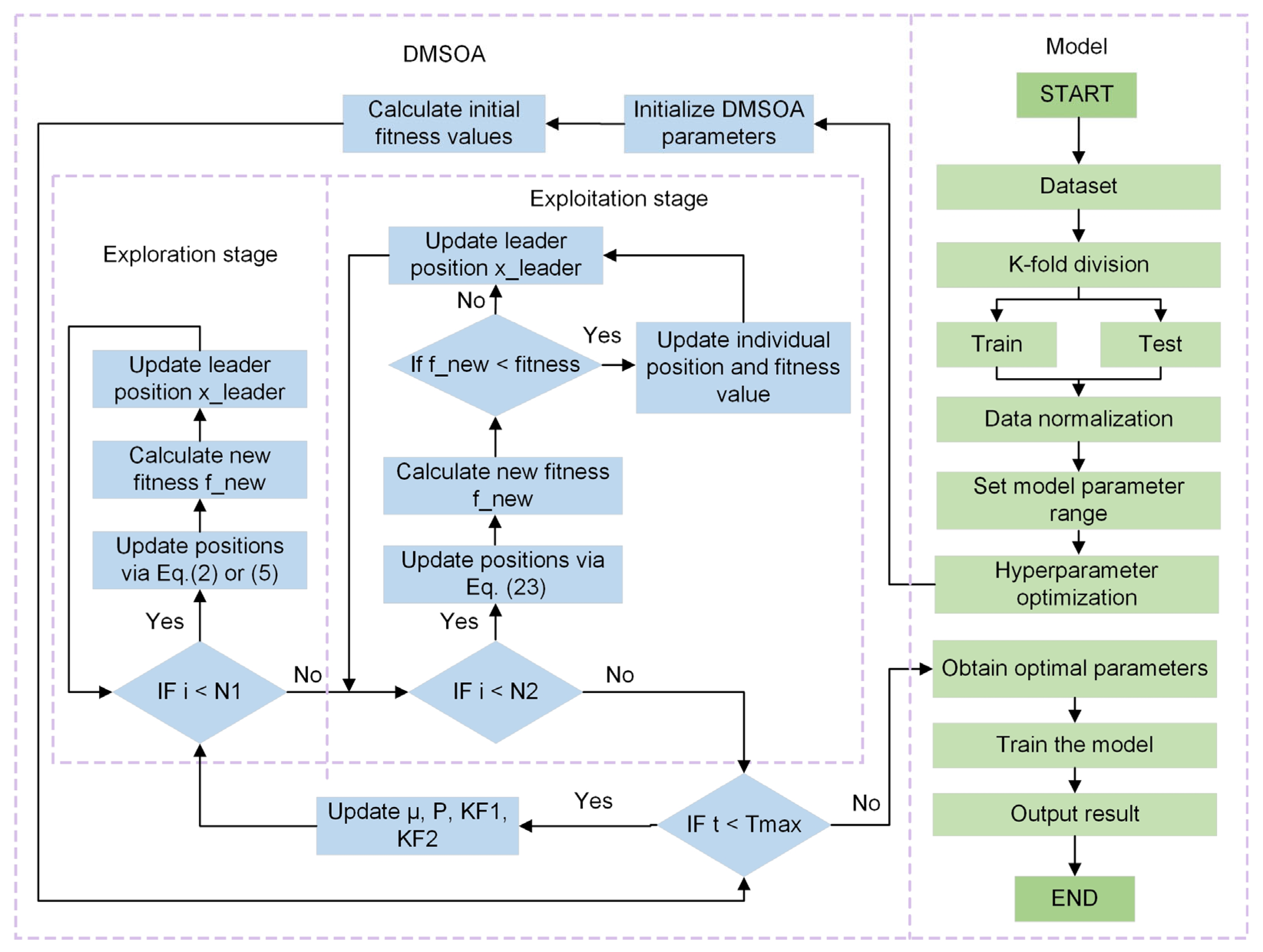
Although intelligent optimisation algorithms have begun to be applied in the prediction of concrete frost resistance, relatively few related studies focus on their utilisation; thus, further exploration is needed. In this paper, a dynamic multi-stage optimisation algorithm (DMSOA) is used to optimise the ensemble learning algorithm to predict the frost resistance of concrete. More than 7090 sets of experimental data are collected, and nine attributes of cement, water, fly ash, coarse aggregate, fine aggregate, mineral powder, water-reducing agent, initial air content of concrete and freeze–thaw cycle times are utilised as input variables. Considering that RF, AdaBoost, CatBoost, and XGBoost are widely used and perform well in relevant studies, this study chooses them to construct benchmark models for comparison. DMSOA and other optimisation algorithms are also used to optimise and establish optimisation models. In addition, all models are evaluated to provide the most accurate prediction model for the frost resistance of concrete. This process not only can greatly save on engineering cost but also has an important guiding significance for engineering design.

2. Method

2.1. Ensemble Learning

Ensemble learning is a method of combining multiple basic models to create robust and accurate models [20], mainly by building and combining multiple learners to solve a single prediction problem. The core concept of the ensemble method is that by combining the predictions of multiple models, it can improve the accuracy and robustness of the prediction, reduce overfitting, and improve the generalisation ability of the model. Ensemble learning is primarily divided into two methods, namely, bagging and boosting. Figure 1 and Figure 2 illustrate its schematic diagrams.
Bagging is a parallel integration method that solves the scattering problem of prediction models by including additional training data [21]. It is primarily used to reduce the variance of model prediction, thereby improving its stability and accuracy. It adds robustness to the final decision by creating multiple models’ ‘integration’; a typical example is the random forest algorithm [22]. In boosting, which trains multiple weak learners in series, each model attempts to correct the errors of the previous model. The key idea of boosting is to combine multiple models with weaker performance into a powerful overall model. Its typical representatives are XGBoost, AdaBoost, and CatBoost.
Bagging emphasizes training multiple models in parallel and averaging their prediction results, which can effectively reduce the volatility of high-variance models. This method is particularly suitable for engineering scenarios such as concrete frost resistance prediction, where issues like measurement errors, data disturbances, or sample imbalance exist, and it can enhance the stability and robustness of the model. Boosting, however, adopts an iterative approach to gradually optimise the residual errors of the previous round of models, making it more applicable to regression tasks with uneven distribution of feature importance and high levels of noise. In the modelling of nonlinear frost resistance indicators involved in this study, boosting can more effectively explore the marginal contributions of weak variables, thereby significantly improving the overall prediction accuracy and model performance.

2.1.1. Random Forest Algorithm

Random forest algorithm is a further development based on bagging, which has high accuracy in classification and regression [23]. As shown in Figure 3, the random forest algorithm introduces ‘randomness of feature selection’ in the training process of the decision tree; that is, at each split decision, instead of selecting the optimal feature from all features, the optimal feature is selected from the random subset of features for splitting. This improvement increases the diversity of the model and improves the generalisation ability whilst effectively reducing the risk of overfitting [24].

2.1.2. Adaptive Lifting Algorithm

AdaBoost is a powerful machine learning meta-algorithm. The core idea is to train a series of weak learners in sequence. These weak learners are typically simple models that learn from multiple attributes of the dataset [25]. Their performance on training data is only slightly better than random guessing. Each learner attempts to correct the errors of its previous learner, and the sample distribution is adjusted in each round so that the previously misscored samples get more attention in the subsequent round, thus gradually improving the performance of the model.

2.1.3. CatBoost Algorithm

CatBoost is an open-source machine learning algorithm developed by Yandex. As shown in Figure 4, it belongs to a variant of gradient lifting decision tree, which optimises the processing of classification features and demonstrates superior performance on multiple standard datasets [26]. The design goal of CatBoost is to improve the training efficiency of the model, reduce the possibility of overfitting, and provide high prediction accuracy.
CatBoost can automatically process categorical variables without additional data preprocessing such as hot coding. It also uses ordered lifting and other complex regularisation techniques to effectively combat the overfitting problem. The symmetric decision tree it constructs simplifies the model and reduces the prediction time of the model.

2.1.4. XGBoost Algorithm

XGBoost is an efficient gradient boosting framework optimised for large-scale and distributed machine learning problems. This algorithm aims to provide a scalable, portable, and efficient gradient lifting solution which can effectively deal with various regression and classification problems by using gradient lifting algorithm and various performance optimisations [27]. The advantage of XGBoost is that it can handle a large amount of sparse data, avoid overfitting through regularisation methods, and improve the generalisation ability of the model. The core algorithm is based on decision tree ensemble, and the approximation of the second derivative is used for quick optimisation.

2.2. Dynamic Multi-Stage Optimisation Algorithm

As shown in Figure 5, the dynamic multi-stage optimisation algorithm (DMSOA) is a group-intelligence-based multi-stage search strategy. The algorithm divides the search process into three stages: initialization, exploration, and exploitation. Through dynamic parameter adjustment, it achieves a smooth transition from early wide exploration to later fine exploitation [28]. During the exploration stage, candidate solutions undergo weighted updates by integrating their own positions with the global optimal position. In the exploitation stage, conditional branching or local relocation is performed based on fitness gains to avoid entrapment in local optima. The algorithm’s multi-strategy collaboration mechanism not only accelerates convergence but also enhances robustness, demonstrating exceptional performance in continuous optimisation, combinatorial scheduling, and constrained problems.
DMSOA combines a phased search mechanism and an adaptive weight adjustment strategy to balance global search and local exploitation capabilities. Compared with existing optimisation algorithms, its main characteristics are as follows:
(1) Dynamic phase switching mechanism: The optimisation process is divided into three stages: initialisation, exploration, and exploitation. Each phase adopts a differentiated update strategy, supporting the dynamic adjustment of search behaviour along with the algorithm’s progress, thereby enhancing global exploration capability and convergence efficiency.
(2) Nonlinear adaptive parameter control: Core parameters decay nonlinearly with the iteration process, enabling a natural transition from rough search to fine search, which helps avoid falling into local optima.
(3) Hybrid perturbation operator mechanism: A combination of perturbation operators is introduced in the local exploitation stage, which enhances the diversity and robustness of local searching and further improves the solution quality and algorithm stability.

2.2.1. Initialisation Stage

The initial goal is to randomly distribute the positions of the candidate solutions in the search space (that is, the initial position of the algorithm). The formula is as follows:
X i = L b + ( U b L b ) r a n d ( )
where X i represents the position of the i -th candidate solution, L b and U b are the lower and upper bounds of the search space, and r a n d ( ) represents returning a random number in the interval of [0, 1].

2.2.2. Exploration Stage

During the exploration phase, the candidate solutions approach the optimal solution at a certain rate, and at the same time, they improve their positioning by self-correction and updating the environmental information (the positions of other candidate solutions). The position update formula for this stage is as follows [27]:
X i t + 1 = X i t + μ X i t s i g n ( r 0.5 ) , P > r a n d X i t + C F 1 ( X l e a d e r t X i t ) + C F 2 ( X j t X i t ) , P r a n d
where X i t and X i t + 1 represent the position of the i -th candidate solution at time t and t + 1 ; X l e a d e r t is the position of the advantage solution at time t; and X j t is the position of the j -th candidate solution (other candidate solution near i -th candidate solution) at time t . The scaling factor µ is a crucial parameter that controls the movement step size of candidate solutions, serving to adjust the speed at which they approach superior solutions. This factor plays a role in balancing global exploration and local exploitation during the search process. A larger value of µ helps expand the search radius and enhance global exploration capability, which is conducive to escaping local optima, while a smaller value of µ promotes refined searching in potential high-quality regions, thereby improving the effect of local optimisation. The scaling factor µ is dynamically decayed with the number of iterations, reflecting the fact that as the algorithm progresses, the search strategy gradually transitions from global exploration to local exploitation. Its calculation method is as follows:
μ = K × ( 1 t / t max )
where K is calculated as:
K = sin ( 2 r a n d ) + 1
After the formula is integrated, it becomes:
X i t + 1 = C 1 μ ( X i t C 2 X l e a d e r t ) sign ( r 0.5 ) + X i t + C F 1 ( X leader t X i t ) + C F 2 ( X j t X i t )
where C 1 and C 2 are the regulation coefficients in the algorithm, and C F 1 and C F 2 are the local search coefficients, which are used to control the interaction between candidate solutions; the s i g n ( r 0.5 ) function determines the search direction based on the value of r (a random number).

2.2.3. Exploitation Stage

During the development stage, the particles perform more precise optimisation based on the area where the best solution is located, thereby further enhancing the overall optimisation performance of the particle swarm. To prevent the algorithm from converging prematurely or falling into local optima, a conditional branching mechanism is introduced, as shown in Equation (6). This conditional switching strategy can effectively prevent the algorithm from getting trapped in local optima. When the current solution performs well, particles will approach the optimal solution with a higher weight to achieve local fine-grained searching; when the current solution performs poorly, differential perturbations between neighbouring solutions are introduced to expand the search range and enhance global exploration capability.
X i t + 1 = μ ( X l e a d e r t X i t ) + X i t , i f   f ( X i t ) > f ( X i t + 1 ) K F 1 ( X l e a d e r t X i t ) + K F 2 ( X k t X j t ) + X i t , o t h e r w i s e
where f ( X i t ) and f ( X i t + 1 ) are the values of the fitness function of the candidate solution at positions X i t and X i t + 1 , respectively, and the fitness function is used to evaluate the merits and disadvantages of each position, usually corresponding to the value of the objective function in the optimisation problem; X k t and X j t are the positions of the other two candidate solutions near the i -th candidate solution at time t , respectively, which are involved in computing a new position update. The two parameters, K F 1 and K F 2 , are coefficients that control local search behaviour and regulate the strength of the advantage solution influence and intragroup interactions, respectively, which help the algorithm balance between the exploration phase and the development phase. The value ranges of C F 1 , C F 2 , K F 1 , and K F 2 are all in (0, 2), and the calculation formula is:
C F i   o r   K F i 1 F P r a n d ( 0 , 1 ) , ( i = 1 , 2 )
where F P is a constant, and the value is 0.618; r a n d is a random number in (0, 1).

3. Data Processing and Analysis

3.1. Data Acquisition

This study uses 7090 datasets, of which 1215 data are derived from the daily experiments of the research group. The laboratory data are measured by the research group through a series of freeze–thaw cycle experiments on concrete samples with different mix proportions through strict experimental procedures. All samples are tested under the same experimental conditions to ensure the consistency and comparability of the data. Another 5875 pieces of data are derived from published related research papers. This part of the data is carefully screened during the collection process, retaining only research results that are consistent with the objectives of this study, with clear data sources and standardised experimental methods. In addition, nine input variables such as cement and water, as well as two prediction indices of relative dynamic elastic modulus and mass loss rate required for this study, are retained. The collected data are divided into two datasets for data processing and analysis. One is relative dynamic elastic modulus (RDEM) as the prediction index, and the other is mass loss rate (MLR) as the prediction index. The input indices are defined as C (cement), W (water), FA (fly ash), S (fine aggregate), G (coarse aggregate), WRA (water reducer), GGBS (mineral powder), GC (gas content), and NFTC (freeze–thaw cycle times). These features are selected based on the widely recognised influencing factors in existing research on concrete frost resistance and engineering practices, covering raw material composition, admixture usage, and environmental acting factors.
Table 1 and Table 2 show the descriptive statistics of variables in the dataset. The statistical indicators, such as minimum value, maximum value, mean value, and standard deviation in the table, reveal the core characteristics of the dataset and comprehensively reflect the variability, concentration trend, and overall distribution range of the data.
To show the relationship among the variables in the dataset, the scatter plot matrices of relative dynamic elastic modulus and mass loss rate are drawn, respectively, as shown in Figure 6 and Figure 7. A scatter plot matrix is a data visualisation tool used to exhibit binary relationships between multiple variables in a single view; it can help identify relationships between variables, distribution patterns of data, and potential outliers [29]. The diagonal graph shows the frequency distribution histogram of the data distribution of a single variable. The upper half of the diagonal shows the joint probability density plot of the two variables. The darker colour indicates denser data points in this area, and the sparse area far away from the main density area may indicate outliers. The graph in the lower half of the diagonal shows a scatter plot of the relationship of the two variables.
To ensure the accuracy of the model and avoid the problem of multicollinearity, the correlation between input variables should be less than 0.8 [30]. To further verify the correlation between the selected features and the prediction indicators, as shown in Figure 8 and Figure 9, a heatmap of Pearson correlation coefficients is used to display the linear relationships between variables. Pearson’s correlation coefficient is a statistical indicator that measures the degree of linear correlation between two variables. When the two variables move in the same direction, the value is positive; when the two variables move in opposite directions, the value is negative. Each grid in Figure 8 and Figure 9 represents the correlation coefficient between the two variables. The range of the coefficient is from −1 to +1. Red represents positive correlation; blue represents negative correlation, and the depth of colour represents the strength of correlation. In Figure 8, RDEM shows a moderate negative correlation with NFTC, and RDEM shows a low correlation with the other parameters FA, GGBS, S, G, WRA, GC, and W. In Figure 9, MLR shows a very strong negative correlation with W, MLR shows a moderate positive correlation with GGBS and WRA, and MLR shows a low correlation with the other following parameters: C, FA, S, G, and GC.

3.2. Data Preprocessing

3.2.1. Data Cleaning

Unprocessed data may contain a variety of problems, which will affect the effectiveness and accuracy of data analysis and model training. Accordingly, the two datasets should be cleaned. The first step is to deal with missing values and duplicates. Given the sufficient samples in the dataset, it is chosen to filter out the data with missing values and duplicates and delete them directly. Then, to improve data quality, outliers are handled. This study adopts the interquartile range (IQR) method to identify and remove outliers: for each numerical variable, the first quartile (Q1) and the third quartile (Q3) are calculated, and then the upper and lower bounds are determined based on 1.5 times the IQR (Q3–Q1) so as to filter out the abnormal sample values beyond this range. Finally, in terms of model selection, the ensemble learning model that is robust to noise and capable of handling nonlinear relationships is used as the benchmark model to deal with the problem of data noise.

3.2.2. Data Standardisation

Data standardisation is an important step in the data preprocessing of machine learning. Its main purpose is to adjust the scale of variables to put them in the same magnitude, thereby improving the performance and efficiency of the algorithm. Here, the dataset is processed using the Z-score normalisation formula in the normalisation process, with the following calculation formula:
X s t d = X μ σ
where X denotes the raw data, μ is the mean of the data, and σ is the standard deviation of the data.

3.2.3. Data Partitioning

To better estimate the average performance of the model, the K-fold cross validation method is chosen in Figure 10 [31]. K-fold cross validation is a technique commonly used in statistical modelling and machine learning. In the process, the entire dataset is randomly divided into k subsets of equal size. During this k training and verification process, one of them will be selected each time. One subset is used as the verification set, and the remaining k−1 subsets are used as the training set to train the model.
In this way, each subset will be used as the primary verification set and k−1 training set. By performing multiple trainings and evaluations on different combinations of training sets and test sets, the model evaluation results are less affected by the contingency of single data segmentation. In this study, k is assigned a value of 10, that is, ten-fold cross-validation.

4. Hyperparameters

4.1. Hyperparameter Selection

In the training process of machine learning models, the selection of hyperparameters is a crucial step which can profoundly affect the performance and prediction accuracy of the model. Appropriate parameter selection can largely improve the model’s ability to fit and generalise data [32]. To establish the performance benchmark and compare it with DMSOA, the manual parameter adjustment is conducted through auxiliary images before DMSOA optimisation so as to roughly determine the applicable hyperparameter ranges for the RF, AdaBoost, CatBoost, and XGBoost models. The manual adjustment process provides a reasonable initial search space for DMSOA optimisation and also ensures the efficiency and effectiveness of the subsequent optimisation process.
A mean square error heat map is a chart used to visualise the relationship between model parameters and their performance. During the hyperparameter tuning process of ensemble learning models, the heat map provides an intuitive way to observe the impact of two different hyperparameter configurations on the prediction error of the model. Both the RF and AdaBoost models select two main hyperparameters, n_estimators (the number of trees or weak learners), and max_depth (the maximum depth of trees or weak learners). After experimental adjustment, the appropriate hyperparameter range is selected. The mean square error heat map of RF regressor and AdaBoost is drawn, as shown in Figure 11, Figure 12, Figure 13 and Figure 14, to demonstrate the influence of the two hyperparameter combinations on the performance of the model. The colour change in the figure indicates the size of MSE, and the colour changes from red to yellow.
The parallel coordinate graph allows the visualisation of multi-dimensional data and is very suitable for displaying the results of multi-parameter configuration. The CatBoost model selects three important parameters: iterations (number of trees), learning_rate (learning rate per iteration), and depth (maximum depth of number). The XGBoost model selects four important parameters, namely, n_estimators (number of trees), learning_rate (learning rate per iteration), gamma (minimum loss reduction when splitting the tree), and max_depth (maximum depth of number). Parallel coordinate plots are drawn, respectively, as shown in Figure 15, Figure 16, Figure 17 and Figure 18, to illustrate the effects of the four parameter combinations of the XGBoost model and the three parameters of the CatBoost model on model performance. Each parameter dimension in the figure has a vertical line, each line represents a parameter and each connecting line represents the result of a parameter combination. The colour change in the line represents the size of MSE. When the colour approaches yellow, the error increases, whereas when the colour approaches purple, the error decreases. When selecting parameters, the connecting line whose colour is biased towards purple should be selected, and the appropriate parameters should be determined through experimental comparison.
Based on the parallel coordinate image analysis, Table 3 and Table 4 show the parameter selection of the RF, AdaBoost, CatBoost, and XGBoost models.

4.2. Hyperparameter Optimisation

A single ensemble learning model typically relies on manual adjustment in the selection of hyperparameters, which have the problems of low efficiency and difficulty in determining the optimal solution. Moreover, the performance of the model is very sensitive to hyperparameters, and incorrect parameter selection may lead to overfitting or underfitting of the model. Therefore, using appropriate optimisation algorithms to systematically explore the parameter space and automatically determine the optimal hyperparameter combination can help improve the accuracy and robustness of the model. Figure 19 shows the flow chart of DMSOA optimising the hyperparameters of the ensemble learning model.
After the dataset is divided into K folds and standardised with Z-score, the search space for the hyperparameters is set. Then, DMSOA automatically performs optimisation through three stages: initialization, exploration, and exploitation. In the initialization stage, candidate solutions are randomly generated within the preset boundaries to initialize the parameters. In the exploration stage, the algorithm performs a global search by updating the positions of the superior individuals, calculating new fitness values, and updating the positions based on the superiority and inferiority. The remaining candidate solutions adjust their positions according to specific criteria. In the exploitation stage, the algorithm focuses on conducting local searches in dominant regions and making fine adjustments to individual positions, thereby further enhancing the convergence efficiency of the model. To avoid prematurely falling into local optima and to enhance the adaptability of the search process, DMSOA introduces a dynamic parameter adjustment mechanism during the exploration and exploitation stages. DMSOA adjusts the search intensity and the interaction between individuals through a series of adjustment coefficients (such as μ, C1, C2, CF1, CF2, etc.). Among them, μ decreases nonlinearly with the number of iterations to facilitate the transition from global to local search scope. Meanwhile, coefficients like CF1 and CF2 are dynamically generated through a random mechanism to govern information exchange and local optimisation behaviours among candidate solutions. The design of these parameters aims to enhance the algorithm’s convergence accuracy and global search capability. The dynamic strategy effectively balances the relationship between global exploration and local exploitation, improving the convergence speed and solution quality while reducing the risk of the algorithm becoming trapped in local optima.

5. Model Evaluation

5.1. Pipeline Automation

Using pipeline automation and simplifying the training process of the model, the complete preprocessing and model training steps are encapsulated into a single object and run through this single interface to ensure that all data preprocessing steps are consistent with all models in the cross-validation of the same segmentation, and the comparative evaluation results of different models after ten cross-validations are output at the end.

5.2. Model Evaluation Indicators

This study uses coefficient of determination (R2), mean square error (MSE), root mean square error (RMSE), mean absolute error (MAE), correlation coefficient (CC), and standard deviation ratio (SDR) as the main evaluation indicators. These evaluation metrics are widely used in relevant studies and can comprehensively reflect the goodness of fit, error level, correlation, and stability of the prediction model from multiple dimensions. In terms of indicator selection, this study also considers other evaluation methods such as symmetric mean absolute percentage error and the Theil index. However, since the dataset of this study is not in the form of percentage or normalised structure, and the main goals are regression accuracy and stability, the above six indicators are finally selected as the comprehensive evaluation criteria. R2 represents the model’s ability to explain data variability. The closer the R2 value is to 1, the better the model fits; MSE is the mean of the square of the difference between the predicted and actual values, providing a square measure of error and helping amplify the impact of larger errors. RMSE is the square root of the mean of the square of the difference between the predicted and actual values, providing a standard measure of error. MAE represents the average of the absolute value of the difference between the predicted and actual values, which is less sensitive to the response to outliers and can provide the average level of error. The lower the values of MSE, RMSE, and MAE, the more significant the model’s advantages in error control and prediction stability. CC measures the degree of linear correlation between the two variables and reflects the strength of the linear relationship between the predicted and actual values. SDR is used to compare the standard deviation of the predicted and actual values to measure the volatility of the prediction accuracy [33]. These indicators jointly evaluate the prediction accuracy and explanatory power of the model from different perspectives. The formula is defined as follows:
R 2 = 1 i = 1 n ( y i y ^ i ) 2 i = 1 n ( y i y ¯ ) 2
M S E = 1 n i = 1 n ( y i y ^ i ) 2
R M S E = 1 n i = 1 n ( y i y ^ i ) 2
M A E = 1 n i = 1 n | y i y ^ i |
C C = ( y i y ¯ ) ( y ^ i y ^ ¯ ) ( y i y ¯ ) 2 ( y ^ i y ^ ¯ ) 2
S D R = s y ^ s y
where y i is the actual value, y ^ i is the predicted value, n is the total number of samples, y i y ^ i is the absolute value of the difference between the actual and predicted values, y ¯ is the average value of the actual value, the numerator is the sum of the square difference between the predicted and actual values, the denominator is the sum of the square difference between the actual and actual mean values, s y ^ is the standard deviation of the predicted value, and s y is the standard deviation of the actual value.

6. Results and Discussion

This study constructs four traditional prediction models and four optimised prediction models to evaluate the performance of the models through the following six indicators: R2, MSE, RMSE, MAE, CC, and SDR ratio. Table 5 and Table 6 show the average performance results of the test set after ten-fold cross-validation. From the two tables, the optimisation model using the DMSOA shows better performance than the traditional model, with lower MSE, RMSE, and MAE values, and higher R2, CC, and SDR values, which indicate that the model with DMSOA has a significant improvement in accuracy and prediction error. Among all models, the DMSOA-CatBoost model shows the best performance, and R2 reached 0.864 and 0.885 on the test set of the two datasets, respectively. Moreover, the prediction results were the most accurate among all models.
In addition, a Taylor diagram is a very efficient graphical representation to characterise the prediction performance of models. It evaluates models by combining multiple statistics, adding intuitiveness to the comparison between models; additionally, it can display statistical information in a single chart that generally needs to be represented by multiple charts [34]. Therefore, to show the predicted results through the models in Table 5 and Table 6 more directly, the paper uses a Taylor diagram to compare the prediction effects of different prediction models in Figure 20 and Figure 21. In the figures, the ratio of the standard deviation of the predicted value to the measured value is the radial distance from the origin. The correlation coefficient between the predicted value and the measured value is the angle in the polar diagram, and the root mean square error is the radial distance from the reference point. The red dashed line in the figure is the standard deviation of the reference data point. The model prediction close to this line has a standard deviation similar to the observed value, which means that the model can capture the variability of the data well. The angles of model points show the degree of correlation between their predicted and actual values, and models with angles close to 1 show high correlations. The dashed grey line represents the contours of the RMSE. Similarly, from the two Taylor diagrams, DMSOA-CatBoost tends to the reference point more and has the most outstanding performance.
Figure 22 and Figure 23 are the comparative line charts of the predicted and true values of the DMSOA-CatBoost model on the relative dynamic elastic modulus and mass loss rate test set at a certain fold in the ten-fold cross-validation. From the figure, the predicted and true values are in good agreement, and the expected effect is achieved [35].
To compare the performance of DMSOA with other well-known optimisation algorithms, the CatBoost model was optimised using DMSOA, the sine cosine algorithm (SCA), and the Archimedean optimisation algorithm (AOA), respectively. After 10-fold cross-validation, the average performance results of different optimisation algorithms on the test set were obtained, as shown in Table 7 and Table 8. The experimental results indicate that DMSOA-CatBoost outperforms the SCA- and AOA-optimised models on both the RDEM and MLR datasets, exhibiting better performance across all average metrics. Among them, the DMSOA-CatBoost model consistently maintains the highest SDR, indicating that it has smaller fluctuations across different folds and demonstrates greater stability and robustness under different data partitions.
In addition, to further verify whether the differences in prediction performance among the optimised algorithm models are statistically significant, the R2 values from the 10-fold cross-validation in the experiment are collected. The Wilcoxon signed-rank test, a non-parametric testing method, is selected to conduct pairwise comparisons of the prediction performance differences between DMSOA-CatBoost and AOA-CatBoost, as well as SCA-CatBoost. The tests are performed at a significance level of α = 0.05. As shown in Table 9 and Table 10, DMSOA-CatBoost is significantly superior to AOA-CatBoost and SCA-CatBoost on both datasets, with all p-values less than 0.05. This indicates that DMSOA-CatBoost has a statistically significant predictive advantage, and the significance results effectively support the superiority of the proposed method.
In the field of machine learning for frost resistance prediction, traditional machine learning models often encounter challenges when faced with complex and dynamically changing datasets, including the need to effectively process large amounts of frequently changing data and the need to deal with possible high-dimensional features and nonlinear relationships. When standard CatBoost is faced with ultra-large-scale datasets or complex scenarios that require fine tuning owing to its huge parameter space and high sensitivity, the parameter optimisation process may no longer become intuitive and efficient, which may easily lead to model overfitting or underfitting. The introduction of DMSOA, with its superior development, detection, and local optimal avoidance ability, not only allows one to determine the best hyperparameters but also to adjust the strategy of feature combination and boundary counting, thus improving the adaptability and robustness of the model in changeable environments and significantly improving the predicting accuracy of concrete frost resistance. Combining the efficient search ability of DMSOA with the high-performance learning algorithm of CatBoost, application of the DMSOA-CatBoost optimisation model can accurately predict the frost resistance of concrete and provide a reliable support and decision-making basis for engineering practice.
Moreover, the research group has made achievements in the prediction of different properties of concrete and the recommendation of proportion and made a complete software system. Figure 24 presents the main interface of system function selection, including frost resistance, strength, electric flux and other properties. Figure 25 presents the interface of frost resistance prediction, which also provides the prediction of relative dynamic elastic modulus and mass loss rate. The prediction model is DMSOA-CatBoost. It provides an efficient and accurate tool for engineers and researchers to optimise the design and preparation process of concrete, which not only improves engineering quality but also substantially reduces material waste and engineering costs whilst contributing to the development of concrete technology.

7. Conclusions

In this paper, a new reliable DMSOA-CatBoost model is developed; this new model can be used to predict the frost resistance of concrete more accurately. In the study, by comparing the four ensemble learning models of RF, AdaBoost, CatBoost, and XGBoost and the four optimisation models of DMSOA-RF, DMSOA-AdaBoost, DMSOA-CatBoost, and DMSOA-XGBoost, DMSOA-CatBoost is found to have the highest prediction accuracy. The R2 of relative dynamic modulus and mass loss rate reached 0.864 and 0.885, respectively, which are 6.40% and 11.15% higher than CatBoost. Compared with other models, the deviation is also much smaller with higher accuracy. It also demonstrates excellent optimisation results in the comparative experiments with other optimisation algorithms. The results of this study not only improve the accuracy of predicting the frost resistance of concrete but also provide a robust and effective modelling framework for the broader field of concrete durability assessment. This model can offer decision support for engineers in evaluating the potential deterioration risks of concrete in freeze–thaw environments, thereby enhancing the efficiency and scientificity of material design, quality control, and long-term service performance assessment.
In the future, we can consider expanding the datasets and increasing the diversity of model training, including climatic conditions in other regions and concrete materials with different compositions, into the research scope to improve the applicability and accuracy of the model and obtain a wider range of application scenarios. Meanwhile, it is necessary to conduct external validation experiments to evaluate the model’s performance in actual engineering environments. To enhance the model’s transparency and engineering acceptability, subsequent research can also introduce model interpretability analysis methods to deeply explore the key factors affecting concrete frost resistance, thereby providing more guiding technical support for engineering practice.

Author Contributions

Conceptualization, X.D. and J.D.; methodology, J.Y.; software, J.Y.; validation, X.D. and J.D.; formal analysis, J.Y.; investigation, J.Y. and X.D.; resources, X.D. and J.D.; data curation, J.Y. and X.D.; writing—original draft preparation, J.Y.; writing—review and editing, J.Y.; visualization, J.Y.; supervision, X.D.; project administration, X.D. and J.D.; funding acquisition, X.D. and J.D. All authors have read and agreed to the published version of the manuscript.

Funding

This research was supported in part by the National Natural Science Foundation of China (Grant No. 52368032, 51808272), the China Postdoctoral Science Foundation (Grant No. 2023M741455), the Tianyou Youth Talent Lift Program of Lanzhou Jiaotong University, the Gansu Province Youth Talent Support Project (Grant No. GXH20210611-10), and in part by the Natural Science Foundation of Gansu Province (Grant No. 23JRRA889) and the Innovation Fund Project of Colleges and Universities in Gansu Province (Grant No. 2024B-057).

Data Availability Statement

The data can be requested from the corresponding author upon reasonable request.

Acknowledgments

The authors would like to thank the technical team of the Key Laboratory of Opto-Electronic Technology and Intelligent Control of the Ministry of Education, Lanzhou Jiaotong University, and the National and Provincial Joint Engineering Laboratory of Road & Bridge Disaster Prevention and Control, Lanzhou Jiaotong University, for their technical support.

Conflicts of Interest

The authors declare no conflicts of interest.

References

  1. Sah, A.K.; Hong, Y.M. Performance comparison of machine learning models for concrete compressive strength prediction. Materials 2024, 17, 2075. [Google Scholar] [CrossRef] [PubMed]
  2. Gan, B.-L.; Zhang, D.-M.; Huang, Z.-K.; Zheng, F.-Y.; Zhu, R.; Zhang, W. Ontology-Driven Knowledge Graph for Decision-Making in Resilience Enhancement of Underground Structures: Framework and Application. Tunn. Undergr. Space Technol. 2025, 163, 106739. [Google Scholar] [CrossRef]
  3. Huang, X.; Wang, S.; Lu, T.; Wu, K.; Li, H.; Deng, W.; Shi, J. Frost durability prediction of rubber concrete based on improved machine learning models. Constr. Build. Mater. 2024, 429, 136201. [Google Scholar] [CrossRef]
  4. Zhu, X.; Bai, Y.; Chen, X.; Tian, Z.; Ning, Y. Evaluation and prediction on abrasion resistance of hydraulic concrete after exposure to different freeze-thaw cycles. Constr. Build. Mater. 2022, 316, 126055. [Google Scholar] [CrossRef]
  5. Craeye, B.; Cockaerts, G.; Kara De Maeijer, P. Improving freeze–thaw resistance of concrete road infrastructure by means of superabsorbent polymers. Infrastructures 2018, 3, 4. [Google Scholar] [CrossRef]
  6. Bian, Y.; Song, F.; Liu, H.; Li, R.; Xiao, C. Study on the performance of basalt fiber geopolymer concrete by freeze-thaw cycle coupled with sulfate erosion. AIP Adv. 2024, 14, 015136. [Google Scholar] [CrossRef]
  7. Wang, C.; Zhang, M.; Pei, W.; Lai, Y.; Dai, J.; Xue, Y.; Sun, J. Frost resistance of concrete mixed with nano-silica in severely cold regions. Cold Reg. Sci. Technol. 2024, 217, 104038. [Google Scholar] [CrossRef]
  8. Liu, S.; Mao, J.; Ding, Y.; Chen, Y.; Zeng, Y.; Ren, J.; Zhu, X.; Xie, R.; Chen, J.; Wang, C. Comparative study on the effect of crystalline agents for improving frost resistance of concrete from the perspective of reaction mechanism. Case Stud. Constr. Mater. 2024, 20, 03386. [Google Scholar] [CrossRef]
  9. He, H.; Gao, L.; Xu, K.; Yuan, J.; Ge, W.; Lin, C.; He, C.; Wang, X.; Liu, J.; Yang, J. A study on the effect of microspheres on the freeze–thaw resistance of EPS concrete. Sci. Eng. Compos. Mater. 2024, 31, 20220241. [Google Scholar] [CrossRef]
  10. Liu, H.; Luo, G.; Wei, H.; Yu, H. Strength, Permeability, and Freeze-Thaw Durability of Pervious Concrete with Different Aggregate Sizes, Porosities, and Water-Binder Ratios. Appl. Sci. 2018, 8, 1217. [Google Scholar] [CrossRef]
  11. Zhou, S.; Wu, C.; Li, J.; Shi, Y.; Luo, M.; Guo, K. Study on the influence of fractal dimension and size effect of coarse aggregate on the frost resistance of hydraulic concrete. Constr. Build. Mater. 2024, 431, 136526. [Google Scholar] [CrossRef]
  12. Du, L.; Zhou, J.; Lai, J.; Wu, K.; Yin, X.; He, Y. Effect of pore structure on durability and mechanical performance of 3D printed concrete. Constr. Build. Mater. 2023, 400, 132581. [Google Scholar] [CrossRef]
  13. Elamary, A.S.; Sharaky, I.A.; Alharthi, Y.M.; Rashed, A.E. Optimizing Shear Capacity Prediction of Steel Beams with Machine Learning Techniques. Arab. J. Sci. Eng. 2024, 49, 4685–4709. [Google Scholar] [CrossRef]
  14. Li, Y.; Jin, K.; Lin, H.; Shen, J.; Shi, J.; Fan, M. Analysis and prediction of freezethaw resistance of concrete based on machine learning. Mater. Today Commun. 2024, 39, 108946. [Google Scholar] [CrossRef]
  15. Tang, Y.; Wu, X.; Chen, H.; Zeng, T. Prediction of the antifreeze of the concrete structure based on random forest and wavelet neural network. IOP Conf. Ser. Earth Environ. Sci. 2020, 552, 012010. [Google Scholar] [CrossRef]
  16. Wang, L.; Zeng, T.; Tao, Y.; Wu, X.; Chen, H. Research on prediction of concrete frost resistance based on random forest. E3S Web Conf. 2021, 237, 03033. [Google Scholar] [CrossRef]
  17. Gao, X.; Yang, J.; Zhu, H.; Xu, J. Estimation of rubberized concrete frost resistance using machine learning techniques. Constr. Build. Mater. 2023, 371, 130778. [Google Scholar] [CrossRef]
  18. Zhang, J.; Cao, Y.; Xia, L.; Zhang, D.; Xu, W.; Liu, Y. Intelligent prediction of the frost resistance of high-performance concrete: A machine learning method. J. Civ. Eng. Manag. 2023, 29, 516–529. [Google Scholar] [CrossRef]
  19. Chen, H.; Cao, Y.; Liu, Y.; Qin, Y.; Xia, L. Enhancing the durability of concrete in severely cold regions: Mix proportion optimization based on machine learning. Constr. Build. Mater. 2023, 371, 130644. [Google Scholar] [CrossRef]
  20. Mungoli, N. Adaptive Ensemble Learning: Boosting Model Performance through Intelligent Feature Fusion in Deep Neural Networks. arXiv 2023, arXiv:2304.02653. [Google Scholar] [CrossRef]
  21. Nasir Amin, M.; Iftikhar, B.; Khan, K.; Faisal Javed, M.; Mohammad AbuArab, A.; Faisal Rehman, M. Prediction model for rice husk ash concrete using AI approach: Boosting and bagging algorithms. Structures 2023, 50, 745–757. [Google Scholar] [CrossRef]
  22. Golafshani, E.; Khodadadi, N.; Ngo, T.; Nanni, A.; Behnood, A. Modelling the compressive strength of geopolymer recycled aggregate concrete using ensemble machine learning. Adv. Eng. Softw. 2024, 191, 103611. [Google Scholar] [CrossRef]
  23. Khan, A.Q.; Naveed, M.H.; Rasheed, M.D.; Miao, P. Prediction of Compressive Strength of Fly Ash-Based Geopolymer Concrete Using Supervised Machine Learning Methods. Arab. J. Sci. Eng. 2024, 49, 4889–4904. [Google Scholar] [CrossRef]
  24. Sun, Y.; Cheng, H.; Zhang, S.; Mohan, M.K.; Ye, G.; De Schutter, G. Prediction & optimization of alkali-activated concrete based on the random forest machine learning algorithm. Constr. Build. Mater. 2023, 385, 131519. [Google Scholar] [CrossRef]
  25. Lee, S.; Nguyen, N.; Karamanli, A.; Lee, J.; Vo, T.P. Super learner machine-learning algorithms for compressive strength prediction of high performance concrete. Struct. Concr. 2023, 24, 2208–2228. [Google Scholar] [CrossRef]
  26. Beskopylny, A.N.; Stel’makh, S.A.; Shcherban’, E.M.; Mailyan, L.R.; Meskhi, B.; Razveeva, I.; Chernil’nik, A.; Beskopylny, N. Concrete Strength Prediction Using Machine Learning Methods CatBoost, k-Nearest Neighbors, Support Vector Regression. Appl. Sci. 2022, 12, 10864. [Google Scholar] [CrossRef]
  27. Sun, Z.; Wang, X.; Huang, H.; Yang, Y.; Wu, Z. Predicting compressive strength of fiber-reinforced coral aggregate concrete: Interpretable optimized XGBoost model and experimental validation. Structures 2024, 64, 106516. [Google Scholar] [CrossRef]
  28. Zhang, M.; Wen, G. Duck swarm algorithm: Theory, numerical optimization, and applications. Clust. Comput. 2024, 27, 6441–6449. [Google Scholar] [CrossRef]
  29. Mai, H.-V.T.; Nguyen, M.H.; Ly, H.-B. Development of machine learning methods to predict the compressive strength of fiberreinforced self-compacting concrete and sensitivity analysis. Constr. Build. Mater. 2023, 367, 130339. [Google Scholar] [CrossRef]
  30. Smith, G.N. Probability and statistics in civil engineering. In Collins Professional and Technical Books; Nichols Publishing Company: New York, NY, USA, 1986; p. 244. [Google Scholar]
  31. Phan, T.D. Practical machine learning techniques for estimating the splitting-tensile strength of recycled aggregate concrete. Asian J. Civ. Eng. 2023, 24, 3689–3710. [Google Scholar] [CrossRef]
  32. Wang, R.; Zhang, J.; Lu, Y.; Huang, J. Towards Designing Durable Sculptural Elements: Ensemble Learning in Predicting Compressive Strength of Fiber-Reinforced Nano-Silica Modiffed Concrete. Buildings 2024, 14, 396. [Google Scholar] [CrossRef]
  33. Kaloop, M.R.; Kumar, D.; Samui, P.; Gabr, A.R.; Hu, J.W.; Jin, X.; Roy, B. Particle Swarm Optimization Algorithm-Extreme Learning Machine (PSO-ELM) Model for Predicting Resilient Modulus of Stabilized Aggregate Bases. Appl. Sci. 2019, 9, 3221. [Google Scholar] [CrossRef]
  34. Zhang, J.; Wang, R.; Lu, Y.; Huang, J. Prediction of Compressive Strength of Geopolymer Concrete Landscape Design: Application of the Novel Hybrid RF–GWO–XGBoost Algorithm. Buildings 2024, 14, 591. [Google Scholar] [CrossRef]
  35. Nikoo, M.; Aminnejad, B.; Lork, A. Fireffy Algorithm-Based Artiffcial Neural Network to Predict the Shear Strength in FRP-Reinforced Concrete Beams. Adv. Civ. Eng. 2023, 2023, 4065287. [Google Scholar] [CrossRef]
Figure 1. Schematic diagram of Bagging.
Algorithms 18 00441 g001
Figure 2. Schematic diagram of boosting.
Algorithms 18 00441 g002
Figure 3. Schematic diagram of random forest.
Algorithms 18 00441 g003
Figure 4. Schematic diagram of CatBoost.
Algorithms 18 00441 g004
Figure 5. Three-stage diagram of DMSOA.
Algorithms 18 00441 g005
Figure 6. Scatter plot matrix (RDEM).
Algorithms 18 00441 g006
Figure 7. Scatter plot matrix (MLR).
Algorithms 18 00441 g007
Figure 8. Thermograph of Pearson correlation coefficient (RDEM).
Algorithms 18 00441 g008
Figure 9. Thermograph of Pearson correlation coefficient (MLR).
Algorithms 18 00441 g009
Figure 10. Schematic diagram of K-fold cross validation.
Algorithms 18 00441 g010
Figure 11. Mean square error thermograph of hyperparameters for RF model (RDEM).
Algorithms 18 00441 g011
Figure 12. Mean square error thermograph of hyperparameters for RF model (MLR).
Algorithms 18 00441 g012
Figure 13. Mean square error thermograph of hyperparameters for AdaBoost model (RDEM).
Algorithms 18 00441 g013
Figure 14. Mean square error thermograph of hyperparameters for AdaBoost model (MLR).
Algorithms 18 00441 g014
Figure 15. Parallel coordinate diagram of hyperparameters for CatBoost model (RDEM).
Algorithms 18 00441 g015
Figure 16. Parallel coordinate diagram of hyperparameters for CatBoost model (MLR).
Algorithms 18 00441 g016
Figure 17. Parallel coordinate diagram of hyperparameters for XGBoost model (RDEM).
Algorithms 18 00441 g017
Figure 18. Parallel coordinate diagram of hyperparameters for XGBoost model (MLR).
Algorithms 18 00441 g018
Figure 19. Flow chart of DMSOA optimisation model parameters.
Algorithms 18 00441 g019
Figure 20. Taylor diagram (RDEM).
Algorithms 18 00441 g020
Figure 21. Taylor diagram (MLR).
Algorithms 18 00441 g021
Figure 22. Comparison of predicted and true values of DMSOA-CatBoost partial data (RDEM).
Algorithms 18 00441 g022
Figure 23. Comparison of predicted and true values of DMSOA-CatBoost partial data (MLR).
Algorithms 18 00441 g023
Figure 24. Main interface of system function selection.
Algorithms 18 00441 g024
Figure 25. Interface of frost resistance prediction.
Algorithms 18 00441 g025
Table 1. Dataset descriptive statistics of relative dynamic elastic modulus.
VariableUnitMinimumMaximumMeanStandard Deviation
Ckg/m3110.00533.00266.0282.64
FAkg/m30.00266.0067.4941.69
GGBSkg/m30.00190.0016.8531.19
Skg/m3530.00994.00743.4880.88
Gkg/m3777.321703.001133.50153.58
WRAkg/m30.0011.511.542.50
GCkg/m30.069.404.321.90
Wkg/m381.00200.00148.8526.93
NFTCtimes0.00400.00138.0692.65
RDEM%43.33107.4188.0512.08
Table 2. Dataset descriptive statistics of mass loss rate.
VariableUnitMinimumMaximumMeanStandard Deviation
Ckg/m361.00450.00249.4292.84
FAkg/m30.00266.0071.7945.01
GGBSkg/m30.00190.0015.4037.10
Skg/m3530.00874.50734.8788.50
Gkg/m3865.001703.001162.96193.19
WRAkg/m30.008.501.572.25
GCkg/m30.069.404.451.79
Wkg/m381.00200.00141.9233.48
NFTCtimes0.00500.00143.0096.46
MLR%−1.536.520.951.24
Table 3. Hyperparameter selection of models (RDEM).
ModelHyperparameterOptimal Values
RFn_estimators140
max_depth11
AdaBoostn_estimators60
max_depth20
CatBoostiterations200
learning_rate0.5
depth10
XGBoostn_estimators400
max_depth5
learning_rate0.4
gamma0.3
Table 4. Hyperparameter selection of models (MLR).
ModelHyperparameterOptimal Values
RFn_estimators130
max_depth15
AdaBoostn_estimators60
max_depth15
CatBoostiterations50
learning_rate0.5
depth5
XGBoostn_estimators300
max_depth10
learning_rate0.4
gamma0.3
Table 5. Evaluation of different models (RDEM).
ModelR2MSERMSEMAECCSDR
RF0.79529.4975.4123.1270.8940.834
AdaBoost0.73438.2746.1563.7850.8620.834
CatBoost0.81226.9585.1772.6290.9010.921
XGBoost0.80428.2185.2862.9060.8980.930
DMSOA-RF0.81227.0075.1702.8890.9030.856
DMSOA-AdaBoost0.79529.3365.4093.1360.8940.857
DMSOA-CatBoost0.86419.7394.3692.4240.9300.924
DMSOA-XGBoost0.85820.7674.4832.5150.9270.918
Table 6. Evaluation of different models (MLR).
ModelR2MSERMSEMAECCSDR
RF0.7880.3210.5620.3120.8900.842
AdaBoost0.7450.3840.6140.3910.8720.879
CatBoost0.7960.3050.5520.2640.8960.908
XGBoost0.7710.3360.5760.3290.8820.838
DMSOA-RF0.7990.3040.5480.3040.8960.854
DMSOA-AdaBoost0.7910.3160.5600.3630.8950.865
DMSOA-CatBoost0.8850.1670.4030.2250.9410.924
DMSOA-XGBoost0.8400.2400.4800.2730.9190.886
Table 7. Evaluation of different optimised models (RDEM).
ModelR2MSERMSEMAECCSDR
SCA-CatBoost0.84221.0564.5902.5620.9210.912
AOA-CatBoost0.85420.1104.4842.4930.9250.918
DMSOA-CatBoost0.86419.7394.3692.4240.9300.924
Table 8. Evaluation of different optimised models (MLR).
ModelR2MSERMSEMAECCSDR
SCA-CatBoost0.8610.1900.4360.2430.9330.914
AOA-CatBoost0.8720.1780.4220.2330.9370.919
DMSOA-CatBoost0.8850.1670.4030.2250.9410.924
Table 9. Wilcoxon signed-rank test results (RDEM).
Model ComparisonStatistic (W)p-ValueSignificance (α = 0.05)
DMSOA-CatBoost vs. SCA-CatBoost00.014
DMSOA-CatBoost vs. AOA-CatBoost50.020
Table 10. Wilcoxon signed-rank test results (MLR).
Model ComparisonStatistic (W)p-ValueSignificance (α = 0.05)
DMSOA-CatBoost vs SCA-CatBoost00.009
DMSOA-CatBoost vs AOA-CatBoost70.017
Disclaimer/Publisher’s Note: The statements, opinions and data contained in all publications are solely those of the individual author(s) and contributor(s) and not of MDPI and/or the editor(s). MDPI and/or the editor(s) disclaim responsibility for any injury to people or property resulting from any ideas, methods, instructions or products referred to in the content.

