Abstract
In this article, we present the extended simple equations method (SEsM) for finding exact solutions to systems of fractional nonlinear partial differential equations (FNPDEs). The expansions made to the original SEsM algorithm are implemented in several directions: (1) In constructing analytical solutions: exact solutions to FNPDE systems are presented by simple or complex composite functions, including combinations of solutions to two or more different simple equations with distinct independent variables (corresponding to different wave velocities); (2) in selecting appropriate fractional derivatives and appropriate wave transformations: the choice of the type of fractional derivatives for each system of FNPDEs depends on the physical nature of the modeled real process. Based on this choice, the range of applicable wave transformations that are used to reduce FNPDEs to nonlinear ODEs has been expanded. It includes not only various forms of fractional traveling wave transformations but also standard traveling wave transformations. Based on these methodological enhancements, a generalized SEsM algorithm has been developed to derive exact solutions of systems of FNPDEs. This algorithm provides multiple options at each step, enabling the user to select the most appropriate variant depending on the expected wave dynamics in the modeled physical context. Two specific variants of the generalized SEsM algorithm have been applied to obtain exact solutions to two time-fractional shallow-water-like systems. For generating these exact solutions, it is assumed that each system variable in the studied models exhibits multi-wave behavior, which is expressed as a superposition of two waves propagating at different velocities. As a result, numerous novel multi-wave solutions are derived, involving combinations of hyperbolic-like, elliptic-like, and trigonometric-like functions. The obtained analytical solutions can provide valuable qualitative insights into complex wave dynamics in generalized spatio-temporal dynamical systems, with relevance to areas such as ocean current modeling, multiphase fluid dynamics and geophysical fluid modeling.
Keywords:
fractional nonlinear partial differential equations; extended Simple equations method (SEsM); generalized SEsM algorithm; time-fractional shallow water-like systems; analytical solutions MSC:
35A24; 35G50
1. Introduction
Over the past two decades, the use of fractional nonlinear partial differential equations (FNPDEs) has gained considerable popularity in the scientific community as a powerful mathematical framework for modeling and analyzing a wide range of complex phenomena observed in the real world. This modeling approach has been successfully applied in numerous scientific fields, including biology and ecology [1,2,3], fluid mechanics [4,5,6,7], finance and economics [8,9,10], engineering [11,12,13], etc. A central direction in the study of FNPDEs is finding and analyzing their exact analytical solutions. Analytical solutions provide deeper insight into the qualitative behavior of the modeled systems and serve as criteria for validating numerical simulations. However, obtaining exact solutions of FNPDEs poses significant mathematical challenges due to the combined complexities introduced by nonlinearity and non-integer order of derivatives.
Two main strategies for obtaining exact solutions of FNPDEs are widely used in the literature. The first approach involves applying appropriate fractional transformations to reduce the original FNPDEs into equivalent systems of nonlinear ordinary differential equations (ODEs) of integer order. Once this reduction is achieved, various well established analytical techniques can be used, such as ansatz-based methods [14,15,16,17,18,19], group analysis [20,21], perturbation techniques [22,23], and decomposition methods [24,25]. Notable among these are the Hirota method [26], the homogeneous balance method [27], the auxiliary equation method [28], the Jacobi elliptic function expansion method [29], the (/G)-expansion method, the F-expansion method, the tanh-function method [30], the first integral method [31], the exponential function method [32], the simplest equation method [33], the modified method of simplest equation [34], etc. We note that the SEsM used in this study has an almost universal character, since most existing methods for obtaining analytical solutions of nonlinear PDEs (whether via integer-order ODEs or specific special functions) are limited to its particular cases, as shown in [35,36].
The second approach relies on standard traveling wave transformations that reduce the original FNPDEs to simpler fractional differential equations, usually fractional ODEs. Analytical solutions to these fractional ODEs are often represented by known special functions such as the Mittag–Leffler function. These functions are also involved in constructing solutions to the original FNPDEs. Within this class of methods, the fractional sub-equation method [37,38,39,40] is particularly prominent. It uses known solutions to fractional versions of Riccati ODEs to construct analytical solutions to the FNPDEs under study.
The extended SEsM presented in this work provides a flexible and unified framework for obtaining analytical solutions to both single FNPDEs and systems of FNPDEs. In its classical form, the SEsM [41,42,43] was designed to find exact solutions to NPDEs. According to the original SEsM algorithm, the analytical solutions of the studied NPDEs are constructed as complex composite functions, which involve one or more simple composite functions that are power series of solutions to one or more simple equations with the same independent variables. In the last few years, an upgrade of the SEsM has been proposed in [44,45,46]. It consists of presenting the analytical solutions of NPDEs (FNPDEs) as composite functions involving the solutions of at least two different simple equations with different independent variables. This extended version of the SEsM was initially proposed in [44], where it was applied to the extended integer-order Korteweg–de Vries (KdV) equation, with the obtained exact solutions being combinations of two simple composite functions that involve the solutions of two different simple equations with different independent variables. To find the analytical solutions in [44], all popular types of first-order ODEs, such as variants of the ODEs of Riccati and Bernoulli and an ODE of Abel of the first order, have been used as simple equations. So far, a similar approach has been proposed only in [47]. It is based on the Kudryashov method and is applied to the integer-order Boussinesq-like system and the integer-order shallow water wave equation. In this study, however, the proposed methodology is limited to using only two specific ODEs (sub-variants of an ODE of Riccati) as simple equations.
Regarding finding exact solutions of systems of FNDEs, two versions of the extended SEsM adapted to systems of FNDEs have recently been proposed in [45,46]. In [45] an extended version of the SEsM was proposed based on the assumption that variables in a spatio-temporal dynamical system modeled by FNPDEs propagate at different velocities. In this framework, exact solutions of the studied system are constructed using simple composite functions formed by solutions of similar or different types of simple equations with distinct independent variables. This version of the extended SEsM was applied to a system of two FNPDEs that models a complex ecological phenomenon. In this way, numerous new exact solutions were derived using different solutions of a set of first-order ODEs. In [46] a different version of the extended SEsM was introduced under the assumption that variables in the system of FNPDEs exhibit synchronized multi-wave behavior. Accordingly, the solutions of the studied system are constructed as complex composite functions involving power series of solutions of two or more different types of simple equations with different independent variables. This version of the extended SEsM was applied to a system of two FNPDEs that models a complex fluid-like process, such as the one considered in the current study. In this way, numerous multi-wave solutions were obtained based on known exact solutions of a set of different second-order ODEs.
Building on both versions given above, in this paper, a generalized algorithm of the extended SEsM for obtaining exact solutions to systems of FNPDEs is proposed. The algorithm offers several variants at each step, allowing the user to select the most appropriate variant depending on the expected wave dynamics in the modeled real-world process. In this study, we demonstrate the effectiveness of this algorithm by its application to time-fractional versions of the models presented in [48]:
and
Equations (1) and (2) are mathematical generalizations inspired by two variants of the classical Boussinesq system, where is a time-fractional number and in Equation (1) is an arbitrary coefficient. It must be noted that while the original Boussinesq models are derived from fundamental fluid dynamics and describe long surface waves in shallow water, the introduction of a fractional time derivatives in Equations (1) and (2) incorporates memory effects and anomalous dispersion. This extension, though deviating from the classical interpretation, remains relevant for modeling more complex hydrodynamic scenarios, such as wave propagation in porous or multiphase environments, where classical assumptions no longer hold.
Below we shall derive exact solutions of Equations (1) and (2) applying two different steps’ variants of the generalized SEsM algorithm regarding the type of the wave transformation introduced and the type of simple equations used. We note that various new exact solutions of a model system similar to Equation (2) were obtained in [46]. However, to derive these analytical solutions, in [46], a different sub-variant of the extended SEsM was applied than the one used in the current study.
2. Preliminaries Relevant to the Present Study
For the convenience of the reader, in this section we present several important statements from [49,50], which clarify some basic aspects in the current study.
2.1. Fractional Derivative via Fractional Difference
Definition 1.
Let denote a continuous (but not necessarily differentiable) function, and let denote a constant discretization span. Define the forward operator by the equality (the symbol means that the left side is defined by the right side).
then the fractional difference of order ϕ, , of is defined by the expression
and its fractional derivative of order ϕ is defined by the limit
2.2. Modified Fractional Riemann–Liouville Derivative
Definition 2.
Refer to the function of Definition 1.
(i) Assume that is a constant K. Then its fractional derivative of order ϕ is
(ii) When is not a constant, then we will set
and its fractional derivative will be defined by the expression
in which, for negative ϕ, one has
whilst for positive ϕ we will set
When ,
In order to find the fractional derivative of compound functions, the following equation holds:
2.3. Taylor’s Series of Fractional Order
Proposition 1.
Assume that he continuous function has a fractional derivative of order . For any positive integer k and for any ϕ, , then the following equality holds:
with the notation
where is the Euler gamma function. Formally, this series can be written
where is the derivative operator with respect to x, and is the Mittag–Leffler function defined by the expression
Remark 1.
This fractional Taylor’s series does not hold with the standard Riemann–Liouville derivative, but it is applied to non-differentiable functions only.
Corollary 1.
Assume that and that has derivatives of order k (integer), . Assume further that has a fractional Taylor’s series of order provided by the expression
Then, integrating this series with respect to h provides
3. Description of the Generalized Algorithm of the Extended Simple Equations Method (SEsM)
In this section, we shall provide a detailed presentation of the generalized SEsM algorithm, highlighting the various capabilities it offers for obtaining different types of complex analytical solutions of systems of FNPDEs. Several variants of this algorithm can be found in previous works [45,46], and we unite and complement them in this article. As it is shown below, unlike the original SEsM algorithm outlined in [41,42,43], we have swapped its first and second steps, incorporating methodological extensions into both steps of the original SEsM algorithm.
Taking into account the problem we set out to solve in this study, we shall demonstrate all the possible steps of the algorithm above mentioned for a system of two FNPDEs with two independent variables:
where D denotes the arbitrary fractional order derivative operator, as superscripts . give its fractional number and subscripts denote time and partial derivatives. Here, and are polynomials of and and its derivatives, respectively, where and are unknown functions.
The generalized extended SEsM algorithm which is adopted for finding exact solutions of FNPDEs includes the following basic steps:
- Construction of the solution of Equation (19). In addition to the known conventional methods for obtaining exact solutions of Equation (19), where such solutions are constructed by power series of the solutions of one simple (auxiliary) equation (or one special function) with the same independent variable for the both system variables in (19), the SEsM provides also several alternative variants:
- Variant 1: Constructing the solution of Equation (19) by single composite functions. These single composite functions can be
- (a)
- With distinct independent variables: This solution variant is applicable to real-world dynamical models of a type (19), where it is expected that the system variables demonstrate different wave behavior and they move with different wave speeds. Thus, a such solution takes the formwhere are generalized wave variables (to be defined in the next step) and are simple composite functions of the formorwhere and are solutions of simple equations (to be selected at a later stage of the algorithm), and are coefficients to be determined later.Remark 2.The simple equations used may have the same analytical form as shown in [45], but they may have a different form. The form of the simple equations used depends on the physical wave characteristics of the real-world system being modeled.
- (b)
- With a single common wave variable: This solution variant is applicable to real-world dynamical models of a type (19), where it is expected that the system variables demonstrate different wave behavior but it is synchronized. For this case, the solution of Equation (19) reduces towhere are again two simple composite functions of the form similar to (21) or (22) that include the solutions of two distinct simple equations but with a common wave variable.Remark 3.When the simple equations used have an identical analytical form, the solution (23) has the same form as that used in all other known methods for finding exact solutions to systems of FNPDEs (NPDES) to date.
- Variant 2: Constructing the solution of Equation (19) by complex composite functions including combinations of at least two single composite functions. The single composite functions can be:
- (a)
- With distinct independent variables: This solution variant is applicable to real-world dynamical models of a type (19), where it is expected that the both system variables can exhibit both a synchronized multi-wave behavior or non-synchronized multi-wave behavior as the different waves move with different speeds. The simplest examples of synchronized multi-wave behavior of the variables of system (19) can be expressed analytically aswhere are again generalized wave variables, and the single composite functions are expressed as follows:where and are solutions of two distinct simple equations that will be defined in Step 3 of the SEsM algorithm.
- (b)
- With a single common wave variable: This solution variant is applicable to real-world dynamical models of a type (19), where it is expected that the system variables demonstrate multi-wave behavior, where the waves propagate with the same speed. In this scenario, . Given this, it is easy to make a change in the wave coordinates in Equations (24)–(33) to obtain analogous variants of analytical solutions of Equation (19) for this specific case. The form of some solution variants in this category approaches the forms of analytical solutions proposed in several similar methodologies in this field.Remark 4.The analytical forms of the single composite functions can be of the same type for the both system variables; i.e., they can include combinations of solutions of simple equations with an identical analytical form. However, they can also include combinations of solutions of different types’ simple equations, as the specific construction forms are determined by the specific physical nature of the model equations.
- Selection of the traveling wave type transformation. To apply the SEsM to Equation (19), it is crucial to define the fractional derivatives in those equations. The choice of fractional derivatives (e.g., Riemann–Liouville, Caputo, conformable, etc.) is essential for accurately modeling wave dynamics and reflecting the system’s physical properties, based on factors like the process nature, boundary conditions, and memory effect interpretation. In this context, the following variants of transformations are possible.
- Variant 1: Use of a fractional transformation. The choice of explicit form of the fractional traveling wave transformation depends on how the fractional derivatives in Equation (19) are defined. Below, the most used fractional traveling wave transformations are selected.
- (a)
- Conformable fractional traveling wave transformation: , defined for conformable fractional derivatives [51];
- (b)
- Fractional complex transform: , defined for modified Riemann–Liouville fractional derivatives [49], which can applied for Caputo fractional derivatives and other fractional derivative types in studied FNPDEs [52].
- (c)
- Some more specific fractional transformations, such as , defined for Beta derivatives; , defined for M-truncated derivatives [53] and others.
In all the cases, the studied FNPDEs are reduced to integer-order nonlinear ODEs. - Variant 2: Use a standard traveling wave transformation. In this case, by introducing a traveling wave ansatz in the selected variant solutions from Step 1, the studied FNPDEs are reduced to fractional nonlinear ODEs.
- Selection of the forms of the used simple equations.
- For Variant 1 of Step 2: The general form of the integer-order simple equations used iswhere the funcions and are defined in Step 1 of the generalized SEsM algorithm, the wave coordinates and are defined in a Variant 1 of the Step 2 of the SEsM algorithm, are the orders of derivatives of and , are the degrees of derivatives in the defining ODEs, are the highest degrees of the polynomials of and in the defining ODEs, and and are the coefficients in the polynomials of and , respectively. By fixing and (at ) in Equation (34), different types integer-order ODEs can be used as simple equations, such as the following:
- –
- (a) ODEs of the first order with known analytical solutions (for example, an ODE of Riccati, an ODE of Bernoulli, an ODE of Abel of the first kind, an ODE of the tanh-function, etc.);
- –
- (b) ODEs of the second order with known analytical solutions (for example elliptic equations of Jaccobi and Weiershtrass and their sub-variants, an ODE of Abel of the second kind, etc.).
- For Variant 2 of Step 2: The general form of the fractional simple equations used iswhere and denote the fractional derivatives of order with respect to the wave coordinates and , which are defined in a Variant 2 of the Step 2 of the SEsM algorithm; are the highest degrees of the polynomials of and in the defining fractional ODEs; and and are the coefficients in the polynomials of and , respectively. By fixing and in Equation (35), several types of fractional ODEs can be used as simple equations, such as a fractional ODE of Riccati (and its sub-variants) and a fractional ODE of Bernoulli.
- Derivation of the balance equations and the system of algebraic equations. The fixation of the explicit form of constructed variant solutions of Equation (19) presented in Step 1 of the SEsM algorithm depends on the balance equations derived. Substitutions of the selected variants from Steps 1, 2, and 3 in Equation (19) lead to obtaining polynomials of the functions and . The coefficients in front of these functions include the coefficients of the solution of the considered FNPDEs, as well as the coefficients of the simple equations used. Analytical solutions of Equation (19) can be extracted only if each coefficient in front of the functions and contains almost two terms. Equating these coefficients to zero leads to formation of a system of nonlinear algebraic equations for each variant chosen according Steps 1, 2, and 3 of the SEsM algorithm.
- Derivation of the analytical solutions. Any non-trivial solution of the algebraic system above mentioned leads to a solution of the studied FNPDEs by replacing the specific coefficients in the corresponding variant solutions, given in Step 1 as well as by changing the traveling wave coordinates chosen by the variants given in Step 2. For simplicity, these solutions are expressed through special functions. For a Variant 1 of the Step 3, these special functions are and , as their explicit forms are determined on the basis of the specific form of the simple equations chosen (For reference, see Equation (34), where and , , , and are defined.). For Variant 2 of Step 3, the special functions are and , whose exact forms are determined by the type of fractional simple equations used (for reference, see Equation (35), where and , , and are defined).
The above-described algorithm in its verbal form can be most intuitively illustrated through the following block diagram.
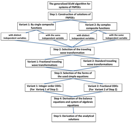
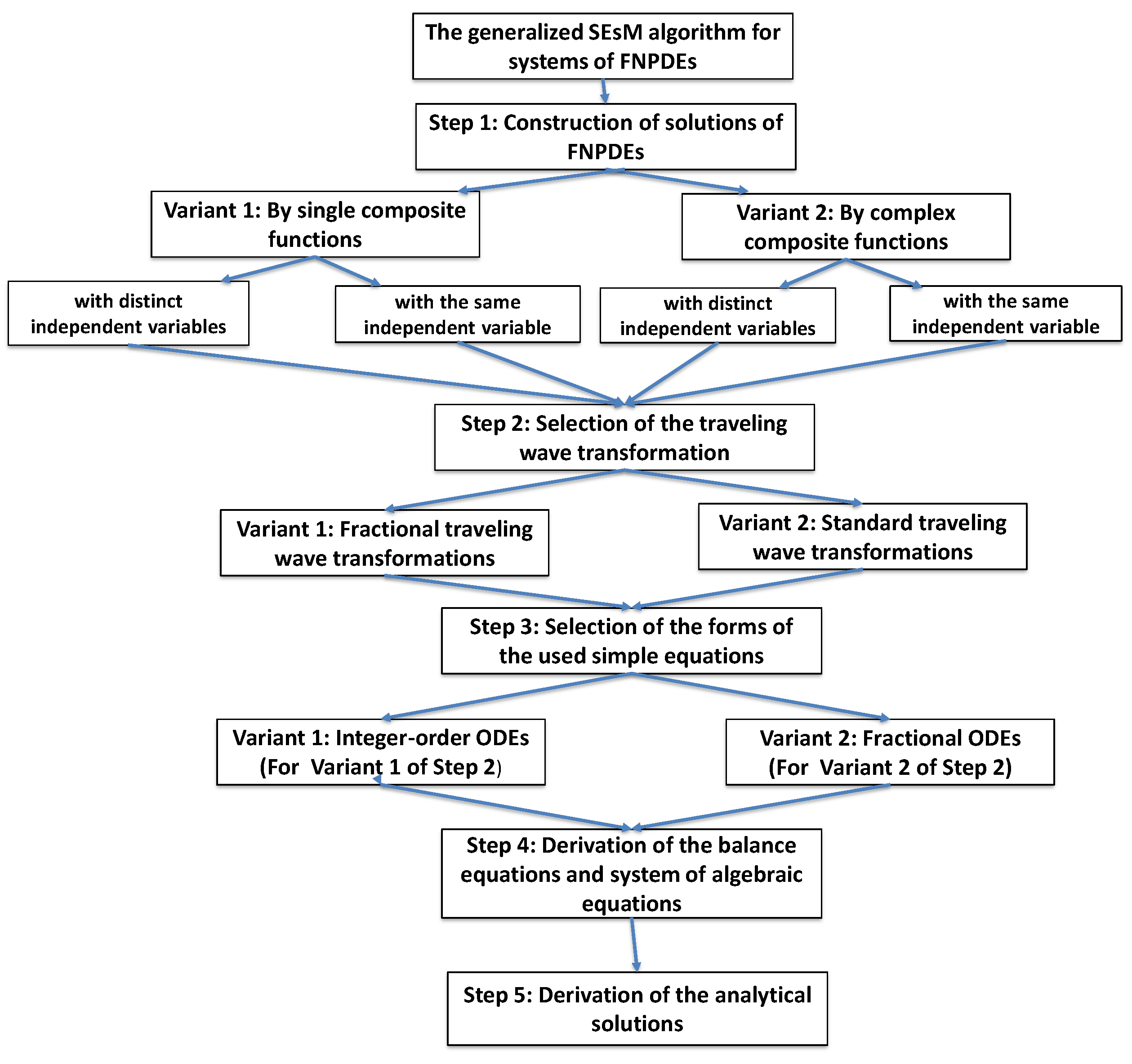
Figure 1.
Block diagram illustrating the generalized SEsM algorithm for systems of FNPDEs.
Figure 1.
Block diagram illustrating the generalized SEsM algorithm for systems of FNPDEs.
The generalized algorithm presented above is designed to support researchers in this field to extract analytical solutions of models of type (19), which describe dynamics of natural processes. Using this algorithm, researchers can select among the variants provided in Steps 1, 2, and 3, making their choice on the basis of the specific characteristics of the wave dynamics which is expected for the natural phenomenon being modeled.
Remark 5.
We briefly outline below how the algorithm can be applied in practice by providing several common heuristic criteria that may assist in selecting the most appropriate variants.
- Nature of wave interactions: Use of composite functions with different independent variables when modeling multi-scale or interacting wave phenomena; Use of a common variable for coherent or synchronized structures.
- Transformations: Fractional traveling wave transformations may be beneficial when standard forms fail to reduce the system effectively or when additional degrees of freedom are required.
- Fractionality: Choose fractional ODEs if the system exhibits pronounced nonlocality or memory effects; otherwise, integer-order ODEs may provide a better approximation.
- Analytical tractability: Simpler variants may be preferred when aiming for closed-form expressions or when the PDE system has known similarity reductions.
4. Derivation of Multi-Wave Exact Solutions of Equation (1) Using a Fractional Wave Transformation
Following the generalized SEsM algorithm, presented above, we choose to present the solution of Equation (1) by complex composite functions, which include sums of two single simple composite functions with different independent variables, i.e.,
Similar to the study conducted in [46], we choose to define Equation (1) in terms of the modified Riemann–Liouville derivative (in the sense of Jumarie), as it is well adapted to modeling nonlocal and memory effects that are prominent in the analysis of the wave dynamics of time-fractional Boussinesq-like systems. The ability of this fractional operator to deal with nondifferentiable functions and its symbolic simplicity make it particularly suitable for constructing exact analytical solutions in this framework. Thus, we introduce the following fractional wave transformations:
We choose to use ODEs of the second order as simple equations. We fix their polynomial parts up to fourth degree, i.e.,
There are many sub-variants of Equation (38) depending on the numerical values of coefficients and . In this study, we chose to fix and . Then, the simple equations used are reduced to
and their analytical solutions (used in this study) are presented in Appendix A.1.
According to Step 4 of the generalized SEsM algorithm, we substitute Equations (36)–(38) in Equation (1). This leads to an equation that includes polynomials of the functions and . We balance the largest degrees of these polynomials. As a result of this balance procedure, the balance equations are and . Then, Equation (36) reduces to
To obtain the system of non-linear algebraic equations, we substitute Equations (37), (39), and (40) in Equation (1). This leads again to an equation that includes polynomials of the functions and . Equating the coefficients in front of these polynomials to 0 leads to the following system of nonlinear algebraic equations:
Thanks to the use of the computer algebra system Maple (https://www.maplesoft.com/ accessed on 30 May 2025), the nonlinear algebraic system (such as Equation (41)) can be solved systematically. The computational process is performed step by step, beginning with the simplest equations and proceeding toward the more complex ones. Although numerous variants of solutions can be generated using symbolic computation, our aim here is to extract those particular solutions in which the coefficients of the constructed solution (as in Equation (40)) are expressed by the coefficients of the simple equations and the coefficients appearing in their respective solutions. One simple non-trivial solution of this system is
where are free parameters.
Then, according to Step 5 of the generalized SEsM algorithm, we present the general solution of Equation (1) by the special functions and as follows:
Substituting the coefficients of Equation (42) in Equation (43) and combining the different analytical solution of Equation (39) leads to the following families of exact solutions of Equation (1):
- Family 1: A solution combined distinct generalized hyperbolic functions with different independent variables.wherefor , andfor . The wave coordinates and are given in Equation (37).
- Family 2: A solution combined distinct generalized trigonometric functions with different independent variables.wherefor , andfor . The wave coordinates and are given in Equation (37).
- Family 3: Solutions combined generalized hyperbolic and trigonometric functions with different independent variables.where is presented in Equation (45) and is presented in Equation (49). The wave coordinates and are given in Equation (37).where is presented in Equation (48) and is presented in Equation (49). The wave coordinates and are given in Equation (37).
- Family 4: Solutions combined generalized elliptic and hyperbolic functions with different independent variables.wherefor . The special function is presented in Equation (46).wherefor . The special function is presented in Equation (46).wherefor . The special function is presented in Equation (46). In all solutions in this paragraph, the wave coordinates and are presented by Equation (37).
- Family 5: Solutions combined generalized elliptic and trigonometric functions with different independent variables.where is presented in Equation (53) and is presented in Equation (49).where is presented in Equation (55) and is presented in Equation (49).where is presented in Equation (57) and is presented in Equation (49). In all the solutions in this paragraph, the wave coordinates and are are presented by Equation (37).

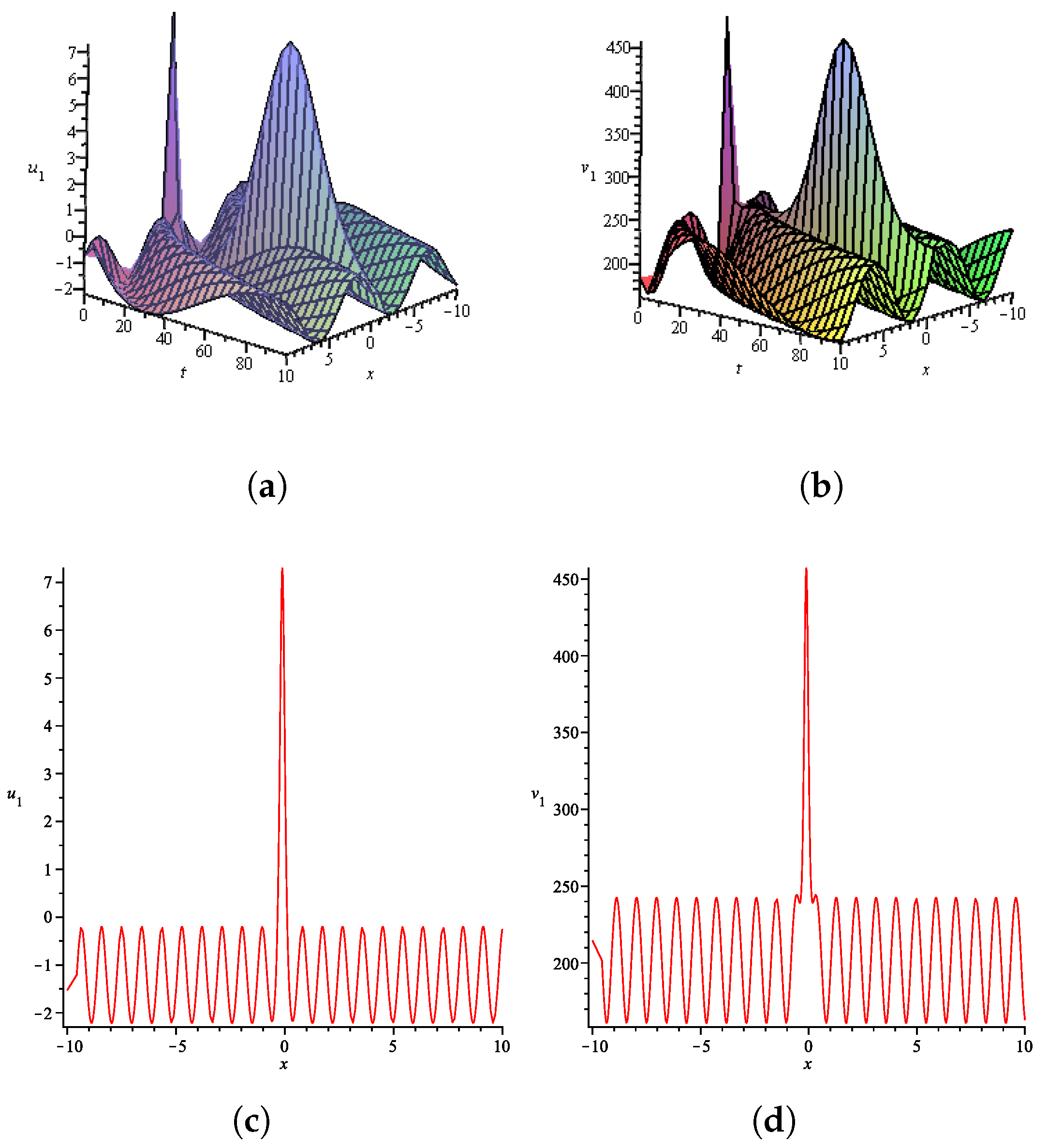
Figure 2.
Numerical simulations of the solution (50) for : 3D plots of (a) u(x,t) and (b) v(x,t); 2D plots of (c) u(x,t) and (d) v(x,t) for .
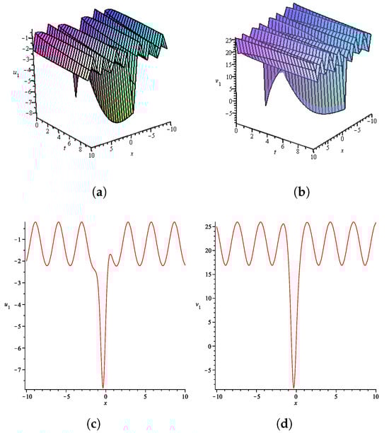
Figure 3.
Numerical simulations of the solution (56) for ; : 3D plots of (a) u(x,t) and (b) v(x,t); 2D plots of (c) u(x,t) and (d) v(x,t) for .
Remark 6.
The hyperbolic, trigonometric, and elliptic functions that appear in the solutions of this section are defined as ‘generalized’ functions with respect to their arguments. It is evident that these arguments include fractional order terms, such as , which reflect the memory and nonlocal effects inherent in fractional calculus. It is obvious that the generalized functions thus defined can easily be reduced to the standard functions when the fractional order , thus restoring the classical (integer-order) case. Therefore, for the particular case , all exact solutions presented above also satisfy the classical (integer-order) version of the system (1).
Remark 7.
When , the exact solutions presented above reduce to those discussed in Step 1 (variant 2b) of the generalized SEsM algorithm; i.e., the distinct types of special functions present in the obtained analytical solutions have the same independent variable. To reach this particular case, it is easy to substitute in Equation (42) and to rewrite all special functions present in the exact solutions of Equation (1) at .
5. Derivation of Multi-Wave Exact Solutions of Equation (2) Using a Standard Traveling Wave Transformation
We present the general solution of Equation (2) again as a combination of two single composite functions including two independent variables:
where the following standard traveling wave transformations are introduced:
We shall use the fractional variants of the ordinary differential equations of Riccati as simple equations:
The analytical solutions of Equation (63) are given in Appendix A.2 and are defined in sense of the modified Jumarie’s Riemann-Liouville derivatives.
Substitution of Equations (61)–(63) in Equation (2) leads to an equation that includes polynomials of the functions and . We balance the largest degrees of these polynomials. As a result of this balance procedure, the balance equations are and . Then, Equation (61) reduces to
To obtain the system of non-linear algebraic equations, we substitute Equations (62)–(64) in Equation (2). This leads again to an equation that includes polynomials of the functions and . Equating the coefficients in front of these polynomials to 0 leads to the following system of nonlinear algebraic equations:
To solve the algebraic system (65) we use the computational software Maple again. There are many analytical solutions to Equation (65) that can be derived using this software, but in this case we choose only one of them. Our motivation for this choice is to relate the coefficients of the solution of Equation (2) to the coefficients of the simple equations used, as well as the coefficients in the traveling wave transform. Thus, one non-trivial solution of Equation (65) is
where are free parameters.
Below we shall present the solution (64) again by special functions and , as follows:
Substituting the coefficients of Equation (66) in Equation (67) and combining the different analytical solutions of Equation (63) leads to the following families of exact solutions of Equation (2):
- Family 3: Solutions combined distinct fractional generalized hyperbolic and trigonometric functions with different independent variables.
- –
- –
- Familly 3. Solutions combained distinct fractional generalized rational (algebraic) functions with different independent variables (when and ).whereIn all the solutions provided in this section, the wave coordinates and are presented by Equation (62)
The fractional generalized trigonometric and hyperbolic functions presented in the most solutions are defined as follows:
where and are Mittag–Leffler functions.
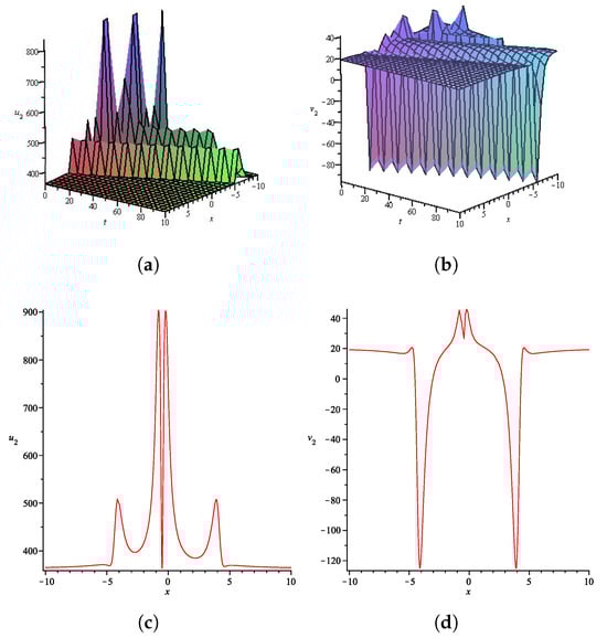
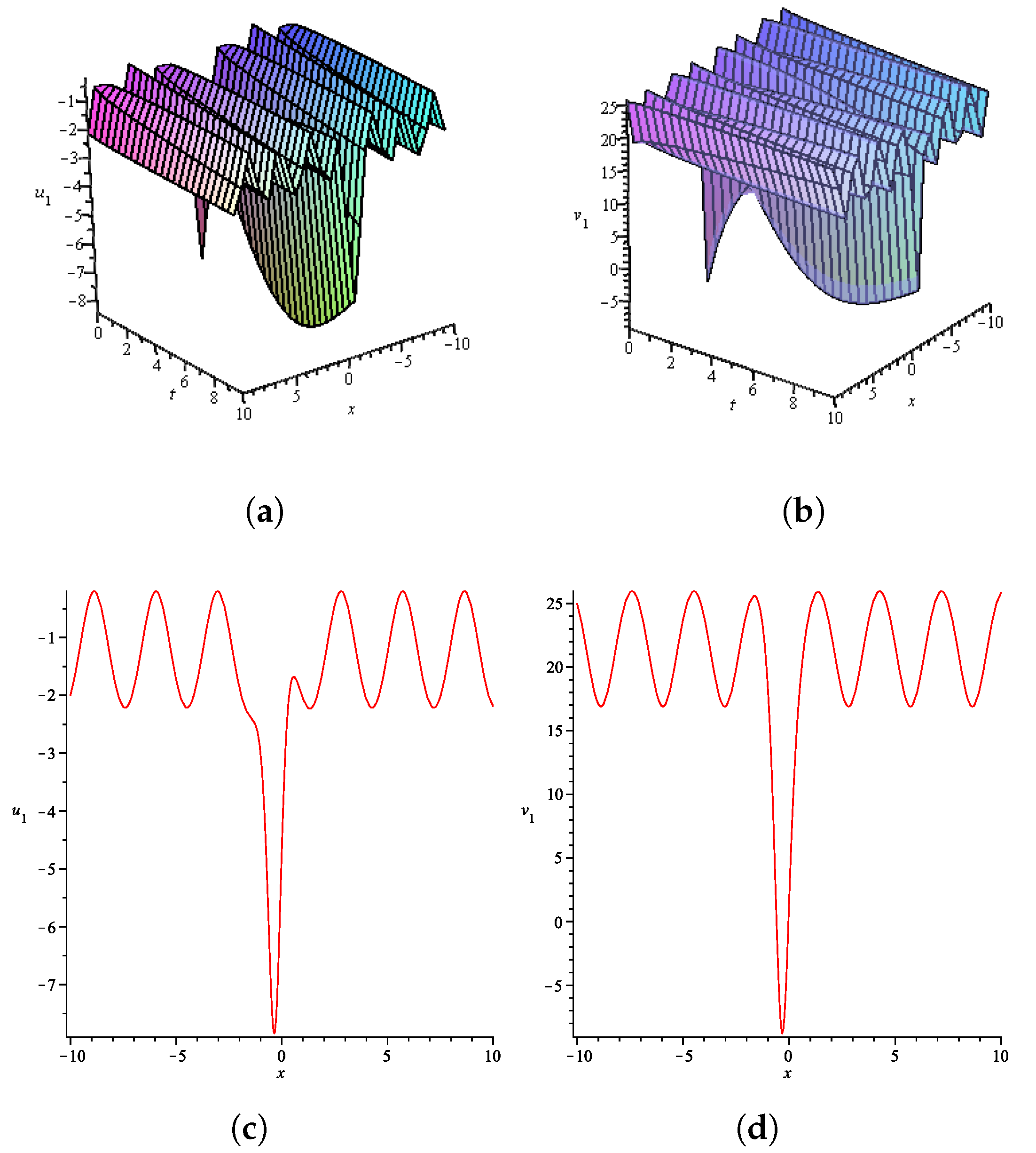
Figure 4.
Numerical simulations of the solution (80) for : 3D plots of (a) u(x,t) and (b) v(x,t); 2D plots of (c) u(x,t) and (d) v(x,t) for .
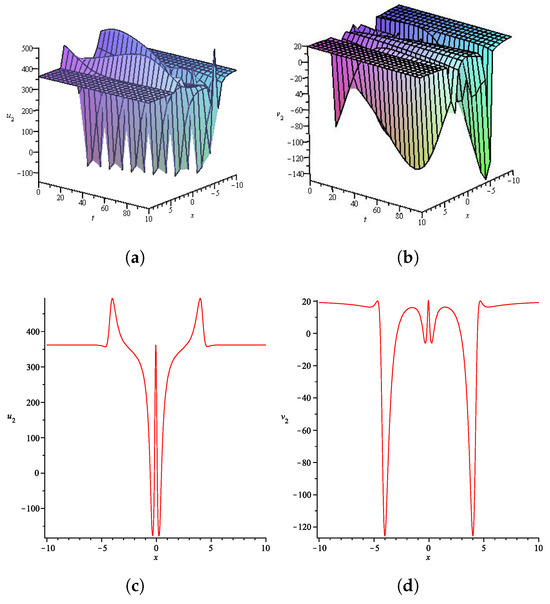
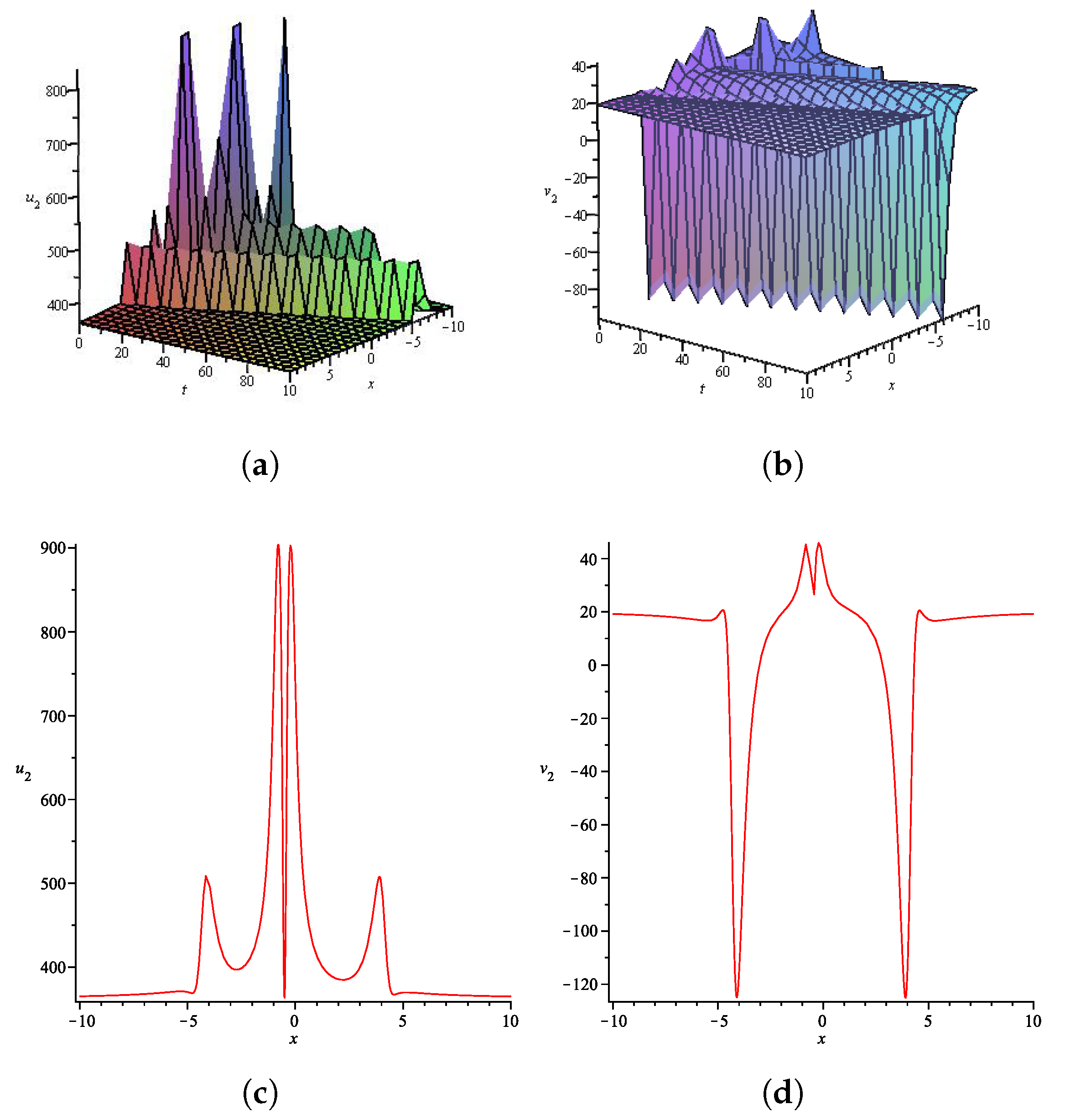
Figure 5.
Numerical simulations of the solution (83) for : 3D plots of (a) u(x,t) and (b) v(x,t); 2D plots of (c) u(x,t) and (d) v(x,t) for .
Remark 8.
The hyperbolic, trigonometric, and rational functions that appear in the solutions of this section are defined as “fractional generalized” functions with respect to the fractional parameter . They differ from the generalized hyperbolic and trigonometric functions of the form that were introduced in the previous section but reduce back to their corresponding classical counterparts at . It is obvious that the fractional generalized functions so defined can easily be reduced to the standard functions when the fractional order , thus restoring the classical (integer) case. Therefore, for the particular case , all the exact solutions presented above also are valid the classical (integer) version of the system (2) at .
Remark 9.
When , the exact solutions presented above reduce to those discussed in Step 1 (variant 2b) of the generalized SEsM algorithm; i.e., the distinct types of special functions present in the obtained analytical solutions have the same independent variable. To achieve this particular case, it is easy to replace in Equation (65) and rewrite all special functions present in the exact solutions of Equation (1) at .
6. Discussion
The choice to construct the analytical solutions presented in Section 4 and Section 5 as combinations (sums) of distinct special functions, such as hyperbolic, trigonometric, or elliptic functions with different independent variables, is motivated by the need to capture richer and more flexible dynamical behavior in the time-fractional Boussinesq-type systems. In contrast to classical (integer-order) models, where solutions typically describe coherent solitary or periodic waves with a single traveling wave velocity, the presence of fractional-order time derivatives introduces memory effects and nonlocal temporal dynamics, which naturally lead to the coexistence of multiple propagation modes with different spatial and temporal scales. Different types of special functions used in the construction of solutions correspond to distinct classes of wave behavior. For example, the hyperbolic functions typically present localized structures such as solitons or traveling fronts, while the trigonometric functions describe regular harmonic oscillations characteristic of linear or weakly nonlinear wave regimes. In addition, the elliptic functions, in turn, capture more complex, anharmonic periodicity and modulated patterns observed in structured or heterogeneous media.
In the same context, the superposition of different functions associated with different wave speeds presented in the analytical solutions derived in Section 4 and Section 5 enables the modeling of interactions between qualitatively different wave structures, such as slowly decaying dispersive waves, rapidly oscillating wave trains, and modulated periodic patterns within a unified analytical framework. The use of hyperbolic and trigonometric functions in combination reflects the interplay between localization and regular periodicity, while combinations involving elliptic functions introduce additional modulation effects, allowing for the description of anharomonic or double-periodic regimes. Notably, the pairing of hyperbolic and elliptic components can model solitary wave fronts modulated by periodic structures, whereas combinations of trigonometric and elliptic functions may represent interference between regular and anharomonic oscillations. This interpretation is supported by the representative solutions visualized in Figure 2, Figure 3, Figure 4 and Figure 5.
Figure 2 shows a solution composed of a hyperbolic and a trigonometric function with different traveling wave variables. The resulting profile exhibits a localized structure superimposed on a regular oscillatory background, illustrating the interaction between solitary and harmonic wave modes. Figure 3 presents a solution constructed from a hyperbolic and an elliptic function with distinct wave variables. The profile shows modulated anharomonic periodicity with a localized deformation, characteristic of complex wave interactions in fractional dispersive media. Figure 4 illustrates a multi-wave solution involving a fractional trigonometric and a fractional hyperbolic function. The surface plots reveal harmonic waves modulated by localized structures, representing multi-scale propagation behavior driven by memory effects. Figure 5 displays another combination of fractional trigonometric and hyperbolic functions, with amplitude-modulated oscillations exhibiting asymmetry and localized energy concentration again indicative of fractional dynamics where distinct wave types coexist and interact.
Therefore, the multi-wave solutions obtained in Section 4 and Section 5 can describe more complex wave processes that may arise from the competition and interaction of different spatial and temporal scales. Although the full physical interpretation of such solutions may be nontrivial, especially for arbitrary fractional orders, we hope that they offer some qualitative insights into the complex behavior of fractional dispersion systems beyond the scope of classical theory.
7. Conclusions
In this paper, a generalized algorithm based on the extended SEsM is proposed for obtaining exact solutions of FNPDEs (in particular, of NPDEs). This algorithm provides several options at each step, which allows the user to choose the most appropriate option depending on the expected wave dynamics in the modeled physical context. One of the main innovations in the proposed algorithm is the ability to construct the exact solutions of the studied FNPDEs by means of composite functions, including solutions of at least two simple equations with different independent variables. Multiple configurations for constructing analytical solutions of systems of type (19) are also shown. The algorithm also includes options for choosing an appropriate wave transform, as well as an appropriate type of ODE in the role of simple equations. In this sense, the SEsM algorithm proposed appears as a generalization (with an extension) of all ansatz-based method algorithms for finding exact solutions of generalized models described by FNPDEs (and as a particular case, by NPDEs).
To demonstrate the wide possibilities provided by the generalized SEsM algorithm, two examples of its application to two variants of a system of NPDEs, which are generalized models of wave dynamics in shallow water processes, are given. To generate exact solutions to both considered systems, it is assumed that each system variable in the studied models exhibits multi-wave behavior, which is expressed as a superposition of two waves propagating at different velocities. In extracting the exact solutions to each studied system of FNPDEs, different wave transformations and different types of simple equations were used. As a result, many new multi-wave solutions were derived, including combinations of generalized hyperbolic, trigonometric, elliptic and rational functions. Numerical illustrations of some of the obtained analytical solutions confirm the analytically presented multi-wave dynamics, expressed in superposition and overlay of various multi-soliton-like and periodic-like waves and packets. It is shown that with minimal mathematical tricks, the analytical solutions obtained in this paper can describe the complex wave dynamics of classical (integer) shallow water models. In this sense, the obtained analytical solutions have a potential application to various scientific fields such as fluid dynamics, geophysics, oceanography and others.
We note that the solutions presented in this paper are only a part of the possible solutions that can be generated by the generalized SEsM algorithm. They are not claimed to be exhaustive in the sense of capturing all possible exact solutions of Equations (1) and (2). For example, with respect to the selected simple Equation (39) in Section 4, all available solutions of the elliptic Jacobi equation, together with its hyperbolic and trigonometric analogues, can also be used to derive additional exact solutions to Equation (1). Furthermore, the solution’s forms to Equation (1) can also include combinations of series of known solutions of different standard ODEs of the first order or mixed combinations of series of known solutions of standard ODEs of the first order and other standard ODEs of the second order. A similar procedure can be applied to find other analytical solutions to Equation (2) too. Furthermore, following Variant 1 of Step 1 in the extended SEsM algorithm, it is possible to construct the solutions of Equations (1) and (2) by distinct simple composite functions, which include the series of solutions of two distinct simple equations with different independent variables for each system variable. However, these and other ideas will be the subject of our future research.
However, it must be noted that the analytical solutions presented in this article are structurally unique with respect to the specific combinations of special functions (e.g., hyperbolic-like, trigonometric-like, elliptic-like functions) and the use of different traveling wave variables. These distinct functional forms and variable dependencies lead to qualitatively different solution types, each representing a specific interaction between propagation modes. This structural uniqueness underlines the diversity and flexibility of the generalized SEsM algorithm.
Finally, it is also of interest to compare the obtained analytical solutions in this article with the solutions obtained by applying accurate numerical methods to Equation (1) and Equation (2). In this way, some validation of the derived analytical solutions here can be achieved. We will realize, however, this idea in a future study.
Funding
This research was supported by the project BG05 M2OP001-1.001-0008 “National Center for Mechatronics and Clean Technologies”, funded by the Operating Program “Science and Education for Intelligent Growth” of the Republic of Bulgaria and the project “Artificial intelligence for investigation and modeling of real processes”, KP-06-H82/4, funded by the Bulgarian National Science Fund.
Data Availability Statement
The original contributions presented in the study are included in the article, further inquiries can be directed to the author.
Conflicts of Interest
The authors declare no conflicts of interest.
Appendix A. Analytical Solutions of the Simple Equations Used in the Paper
Appendix A.1. Analytical Solutions of the Simple Equations Used in Section 4
The equation admits the following solutions [48]:
- A hyperbolic solutionfor and ;
- A trigonometric solutionfor and ;
- Jacobi elliptic function solutions:for ;for ;for where m is a modulus. The Jacobi elliptic functions are doubly periodical and possess properties of triangular functions. Additionally, we note that when , the Jacobi functions degenerate to the hyperbolic functions, i.e.,When , the Jacobi functions degenerate to the triangular functions, i.e.,Additional sub-variants of the elliptic solutions can be found in [54].
The equation admits the following solutions [48]:
- A hyperbolic solutionfor ;
- A trigonometric solutionfor .
Appendix A.2. Analytical Solutions of the Simple Equations Used in Section 5
The equation (or ) admits the following solutions [37]:
- for ;
- for ;
- for ;
- for ;
- for and ,
where
where is a Mittag–Leffler function.
References
- Rivero, M.; Trujillo, J.J.; Vázquez, L.; Velasco, M.P. Fractional dynamics of populations. Appl. Math. Comput. 2011, 218, 1089–1095. [Google Scholar] [CrossRef]
- Owolabi, K.M. High-dimensional spatial patterns in fractional reaction-diffusion system arising in biology. Chaos Solitons Fractals 2020, 134, 109723. [Google Scholar] [CrossRef]
- Ghanbari, B.; Günerhan, H.; Srivastava, H.M. An application of the Atangana-Baleanu fractional derivative in mathematical biology: A three-species predator-prey model. Chaos Solitons Fractals 2020, 138, 109910. [Google Scholar] [CrossRef]
- Kulish, V.V.; Lage, J.L. Application of fractional calculus to fluid mechanics. J. Fluids Eng. 2002, 124, 803–806. [Google Scholar] [CrossRef]
- Yıldırım, A. Analytical approach to fractional partial differential equations in fluid mechanics by means of the homotopy perturbation method. Int. J. Numer. Methods Heat Fluid Flow 2010, 20, 186–200. [Google Scholar] [CrossRef]
- Hosseini, V.R.; Rezazadeh, A.; Zheng, H.; Zou, W. A nonlocal modeling for solving time fractional diffusion equation arising in fluid mechanics. Fractals 2022, 30, 2240155. [Google Scholar] [CrossRef]
- Ozkan, E.M. Exact Solutions of Some Important Nonlinear Fractional Partial Differential Equations with Beta Derivative. Fractal Fract. 2022, 6, 173. [Google Scholar] [CrossRef]
- Fallahgoul, H.; Focardi, S.; Fabozzi, F. Fractional Calculus and Fractional Processes with Applications to Financial Economics: Theory and Application; Academic Press: Cambridge, MA, USA, 2016. [Google Scholar]
- Ara, A.; Khan, N.A.; Razzaq, O.A.; Hameed, T.; Raja, M.A.Z. Wavelets optimization method for evaluation of fractional partial differential equations: An application to financial modelling. Adv. Differ. Equ. 2018, 2018, 8. [Google Scholar] [CrossRef]
- Tarasov, V.E. On history of mathematical economics: Applicatioactionaln of fr calculus. Mathematics 2019, 7, 509. [Google Scholar] [CrossRef]
- Kumar, S. A new fractional modeling arising in engineering sciences and its analytical approximate solution. Alex. Eng. J. 2013, 52, 813–819. [Google Scholar] [CrossRef]
- Sun, H.; Zhang, Y.; Baleanu, D.; Chen, W.; Chen, Y. A new collection of real world applications of fractional calculus in science and engineering. Commun. Nonlinear Sci. Numer. Simul. 2018, 64, 213–231. [Google Scholar] [CrossRef]
- Chen, W.; Sun, H.; Li, X. Fractional Derivative Modeling in Mechanics and Engineering; Springer Nature: Berlin/Heidelberg, Germany, 2022. [Google Scholar]
- Wang, M.; Li, X.; Zhang, J. The (G’/G)-expansion method and travelling wave solutions of nonlinear evolution equations in mathematical physics. Phys. Lett. A 2008, 372, 417–423. [Google Scholar] [CrossRef]
- Zhang, J.; Li, Z. The F–expansion method and new periodic solutions of nonlinear evolution equations. Chaos Solitons Fractals 2008, 37, 1089–1096. [Google Scholar] [CrossRef]
- Kudryashov, N.A. Simplest Equation Method to Look for Exact Solutions of non-linear Differential Equations. Chaos Solitons Fractals 2005, 24, 1217–1231. [Google Scholar] [CrossRef]
- Wazwaz, A.M. The tanh method for traveling wave solutions of nonlinear equations. Appl. Math. Comput. 2004, 154, 713–723. [Google Scholar] [CrossRef]
- Vitanov, N.K. Application of Simplest Equations of Bernoulli and Riccati Kind for Obtaining Exact Traveling-Wave Solutions for a Class of PDEs with Polynomial non-linearity. Commun. Non-Linear Sci. Numer. Simul. 2010, 15, 2050–2060. [Google Scholar] [CrossRef]
- Vitanov, N.K. Modified Method of Simplest Equation: Powerful Tool for Obtaining Exact and Approximate Traveling-Wave Solutions of non-linear PDEs. Commun. Non-Linear Sci. Numer. Simul. 2011, 16, 1176–1185. [Google Scholar] [CrossRef]
- Olver, P.J. Applications of Lie Groups to Differential Equations; Springer: Berlin/Heidelberg, Germany, 1986. [Google Scholar]
- Ibragimov, N.H. CRC Handbook of Lie Group Analysis of Differential Equations, Volumes I–III; CRC Press: Boca Raton, FL, USA, 1994. [Google Scholar]
- Kevorkian, J.; Cole, J.D. Multiple Scale and Singular Perturbation Methods; Springer: Berlin/Heidelberg, Germany, 1996. [Google Scholar]
- Nayfeh, A.H. Introduction to Perturbation Techniques; John Wiley & Sons: Hoboken, NJ, USA, 1981. [Google Scholar]
- Adomian, G.A. review of the decomposition method in applied mathematics. J. Math. Anal. Appl. 1990, 135, 501–544. [Google Scholar] [CrossRef]
- Duan, J.S.; Rach, R. New higher-order numerical one-step methods based on the Adomian and the modified decomposition methods. Appl. Math. Comput. 2011, 218, 2810–2828. [Google Scholar] [CrossRef]
- Hirota, R. Exact Solution of the Korteweg-de Vries Equation for Multiple Collisions of Solitons. Phys. Rev. Lett. 1971, 27, 1192–1194. [Google Scholar] [CrossRef]
- Wang, M.; Zhou, Y. The Homogeneous Balance Method and Its Application to Nonlinear Equations. Chaos Solitons Fractals 1996, 7, 2047–2054. [Google Scholar] [CrossRef]
- Jiong, S. Auxiliary equation method for solving nonlinear partial differential equations. Phys. Lett. A 2003, 309, 387–396. [Google Scholar] [CrossRef]
- Liu, S.K.; Fu, Z.T.; Liu, S.D.; Zhao, Q. Jacobi Elliptic Function Expansion Method and Periodic Wave Solutions of Nonlinear Wave Equations. Phys. Lett. A 2001, 289, 69–74. [Google Scholar] [CrossRef]
- Fan, E. Extended tanh-function method and its applications to nonlinear equations. Phys. Lett. A 2000, 277, 212–218. [Google Scholar] [CrossRef]
- Feng, Z. The First Integral Method to Study the Burgers–KdV Equation. J. Phys. A Math. Gen. 2002, 35, 343–349. [Google Scholar] [CrossRef]
- He, J.H.; Wu, X.H. Exp-Function Method for Nonlinear Wave Equations. Chaos Solitons Fractals 2006, 30, 700–708. [Google Scholar] [CrossRef]
- Kudryashov, N.A.; Loguinova, N.B. Extended Simplest Equation Method for non-linear Differential Equations. Appl. Math. Comput. 2008, 205, 361–365. [Google Scholar] [CrossRef]
- Vitanov, N.K. On Modified Method of Simplest Equation for Obtaining Exact and Approximate Solutions of non-linear PDEs: The Role of the Simplest Equation. Commun. Non-Linear Sci. Numer. Simul. 2011, 16, 4215–4231. [Google Scholar] [CrossRef]
- Vitanov, N.K.; Dimitrova, Z.I.; Vitanov, K.N. Simple Equations Method (SEsM): Algorithm, Connection with Hirota Method, Inverse Scattering Transform Method, and Several Other Methods. Entropy 2021, 23, 10. [Google Scholar] [CrossRef]
- Vitanov, N.K. The Simple Equations Method (SEsM) For Obtaining Exact Solutions Of non-linear PDEs: Opportunities Connected to the Exponential Functions. AIP Conf. Proc. 2019, 2159, 030038. [Google Scholar] [CrossRef]
- Zhang, S.; Zhang, H.-Q. Fractional sub-equation method and its applications to nonlinear fractional PDEs. Phys. Lett. A 2011, 375, 1069–1073. [Google Scholar] [CrossRef]
- Guo, S.; Mei, L.; Li, Y.; Sun, Y. The improved fractional sub-equation method and its applications to the space-time fractional differential equations in fluid mechanics. Phys. Lett. A 2012, 376, 407–411. [Google Scholar] [CrossRef]
- Lu, B. Backlund transformation of fractional Riccati equation and its applications to nonlinear fractional partial differential equations. Phys. Lett. A 2012, 376, 2045–2048. [Google Scholar] [CrossRef]
- Zheng, B.; Wen, C. Exact solutions for fractional partial differential equations by a new fractional sub-equation method. Adv. Differ. Equ. 2013, 2013, 199. [Google Scholar] [CrossRef]
- Vitanov, N.K.; Dimitrova, Z.I.; Vitanov, K.N. On the Use of Composite Functions in the Simple Equations Method to Obtain Exact Solutions of Nonlinear Differential Equations. Computation 2021, 9, 104. [Google Scholar] [CrossRef]
- Vitanov, N.K. Simple Equations Method (SEsM): An Effective Algorithm for Obtaining Exact Solutions of Nonlinear Differential Equations. Entropy 2022, 24, 1653. [Google Scholar] [CrossRef]
- Vitanov, N.K. On the Method of Transformations: Obtaining Solutions of Nonlinear Differential Equations by Means of the Solutions of Simpler Linear or Nonlinear Differential Equations. Axioms 2023, 12, 1106. [Google Scholar] [CrossRef]
- Nikolova, E.V. Exact Travelling-Wave Solutions of the Extended Fifth-Order Korteweg-de Vries Equation via Simple Equations Method (SEsM): The Case of Two Simple Equations. Entropy 2022, 24, 1288. [Google Scholar] [CrossRef]
- Nikolova, E.V. On the Extended Simple Equations Method (SEsM) and Its Application for Finding Exact Solutions of the Time-Fractional Diffusive Predator–Prey System Incorporating an Allee Effect. Mathematics 2025, 13, 330. [Google Scholar] [CrossRef]
- Nikolova, E.V.; Chilikova-Lubomirova, M. Numerous Multi-Wave Solutions of the Time-Fractional Boussinesq-like System via a Variant of the Extended Simple Equations Method (SEsM). Mathematics 2025, 13, 1029. [Google Scholar] [CrossRef]
- Zhou, J.; Ju, L.; Zhao, S.; Zhang, Y. Exact Solutions of Nonlinear Partial Differential Equations Using the Extended Kudryashov Method and Some Properties. Symmetry 2023, 15, 2122. [Google Scholar] [CrossRef]
- Fan, E.; Hon, Y.C. A series of travelling wave solutions for two variant Boussinesq equations in shallow water waves. Chaos Solitons Fractals 2003, 15, 559–566. [Google Scholar] [CrossRef]
- Jumarie, G. Modified Riemann-Liouville derivative and fractional Taylor series of non-differentiable functions further results. Comput. Math. Appl. 2006, 51, 1367–1376. [Google Scholar] [CrossRef]
- Jumarie, G. Table of some basic fractional calculus formulae derived from a modified Riemann-Liouville derivative for non-differentiable functions. Appl. Math. Lett. 2009, 22, 378–385. [Google Scholar] [CrossRef]
- Khalil, R.; Al Horani, M.; Yousef, A.; Sababheh, M. A new definition of fractional derivative. J. Comput. Appl. Math. 2014, 264, 65–70. [Google Scholar] [CrossRef]
- Li, Z.-B.; He, J.-H. Fractional Complex Transform for Fractional Differential Equations. Math. Comput. Appl. 2010, 15, 970–973. [Google Scholar] [CrossRef]
- Riaz, M.B.; Awrejcewicz, J.; Jhangeer, A. Optical Solitons with Beta and M-Truncated Derivatives in Nonlinear Negative-Index Materials with Bohm Potential. Materials 2021, 14, 5335. [Google Scholar] [CrossRef]
- Ebaid, A.; Aly, E.H. Exact solutions for the transformed reduced Ostrovsky equation via the F-expansion method in terms of Weierstrass-elliptic and Jacobian-elliptic functions. Wave Motion 2012, 49, 296–308. [Google Scholar] [CrossRef]

Disclaimer/Publisher’s Note: The statements, opinions and data contained in all publications are solely those of the individual author(s) and contributor(s) and not of MDPI and/or the editor(s). MDPI and/or the editor(s) disclaim responsibility for any injury to people or property resulting from any ideas, methods, instructions or products referred to in the content. |
© 2025 by the author. Licensee MDPI, Basel, Switzerland. This article is an open access article distributed under the terms and conditions of the Creative Commons Attribution (CC BY) license (https://creativecommons.org/licenses/by/4.0/).