Article

The True Shortest Path of Obstacle Grid Graph Is Solved by SGP Vertex Extraction and Filtering Algorithm

School of Artificial Intelligence and Computer Science, Jiangnan University, Wuxi 214126, China
*
Author to whom correspondence should be addressed.
Algorithms 2025, 18(7), 400; https://doi.org/10.3390/a18070400
Submission received: 26 May 2025 / Revised: 22 June 2025 / Accepted: 27 June 2025 / Published: 29 June 2025
(This article belongs to the Section Combinatorial Optimization, Graph, and Network Algorithms)

Abstract

In the obstacle grid map, due to the limitations in search direction imposed by classical path algorithms and meta-heuristic algorithms, the shortest paths are not the true shortest paths (TSPs) but rather the shortest grid paths (SGPs). This paper introduces an SGP vertex extraction and filtering algorithm (SGPVEFA) that identifies key nodes within SGPs. After screening, these nodes yield TSPs under the same conditions. Through various experiments, the shortest path length searched by the SGPVEFA proposed in this paper can be used to search for the real shortest path, and it also has advantages in comparison with recent new algorithms. With the increase in map scale and obstacle rate, the advantages of this path algorithm are more significant.

1. Introduction

The shortest path problem is a fundamental issue in graph theory, with various types. Depending on whether there are constraints, it can be categorized into unconstrained and constrained shortest path problems. For instance, the Vehicle Routing Problem (VPR) is a typical example of a constrained shortest path problem [1]. Based on the number of objectives, it can be divided into single-objective and multi-objective shortest path problems. The Traveling Salesman Problem is a classic example of a multi-objective shortest path problem [2]. Additionally, based on whether the constraints change, it can be classified as static or dynamic shortest path problems, among others. The concept of the shortest path is not limited to physical distance; it can also apply to any quantifiable weight, such as time or cost. In practical applications, many problems can be transformed into shortest path problems for solution.
In path planning, the length of a path is typically the most critical metric, as it directly impacts the cost associated with the path. In general, a shorter path also has fewer waypoints and turns, because the line segments directly connecting the waypoints are the shortest, which means the path is smoother. In robot or vehicle path planning, paths with fewer turns generally consume less energy [3]. Therefore, finding a shorter, collision-free path is a significant challenge.
Currently, algorithms for solving the shortest path problem can be broadly categorized into classical path algorithms and heuristic path algorithms. Classical path algorithms are primarily used to address small-scale deterministic problems, such as Breadth-First Search (BFS), Dijkstra [4], and Depth-First Search (DFS). These algorithms excel in solving problems with a unique optimal solution. Heuristic path algorithms, on the other hand, are more commonly used to tackle large-scale complex problems, including Genetic Algorithms (GA) [5], Ant Colony Optimization (ACO) [6], and Particle Swarm Optimization (PSO) [7]. These algorithms are particularly effective in solving problems with multiple constraints and multi-objective issues [8]. Heuristic algorithms can also be classified into several types based on their principles: population-based algorithms, physics-based algorithms, and evolutionary algorithms [9,10,11].
In recent years, research on the shortest path problem has been prolific. For example, Ref. [12] models real-world problems as weighted time path graphs and proposes a graph transformation technique based on BFS and Dijkstra’s algorithm to study the shortest time paths in these graphs. Ref. [13] utilizes the strategy of Dijkstra’s algorithm to propose a baseline algorithm, which combines the lower bound of the shortest path and the lower bound of the multi-path to develop a framework for solving the K shortest path problem, capable of identifying the first k distinct shortest paths in a directed weighted graph. Ref. [14] introduces a novel genetic algorithm to address the clustering shortest path tree problem (CluSPTP) and tests it on both Euclidean and non-Euclidean instance sets. Ref. [15] proposes an improved distance-based ant colony optimization path (IDBACOR), incorporating direction information into the pheromone update process and adding a speed factor to the probability calculation, guiding ants to move towards the target point as much as possible, thereby solving the shortest path problem in transportation networks.
However, in the context of two-dimensional obstacle grid maps, some existing algorithms struggle to find optimal solutions. Classic pathfinding algorithms, such as BFS and Dijkstra, are limited to searching in four or eight directions, which means they do not always find the true shortest path (TSP) but rather the shortest grid path (SGP) [16,17]. The second chapter of this paper explains the differences between these two types of paths. Heuristic pathfinding algorithms, such as GA, ACO, and PSO, can break through the search direction limitations in close-range scenarios, finding shorter paths than classic pathfinding algorithms. However, when the distance between the start and end points is too large, the efficiency of heuristic pathfinding algorithms significantly decreases, and their solution quality may even fall short of that of classic pathfinding algorithms. Although [16] has shown that the ratio of SGPs to TSPs is limited within a certain range, as the map expands and the distance between the start and end points increases, there can still be a significant gap between SGPs and TSPs. Previous research has also attempted to overcome the search angle limitations to shorten path lengths. For example, Ref. [18] proposed a variant of A* algorithm, aimed at finding paths shorter than the SGP. Ref. [19] introduced an Any-angle pathfinding (Anya) algorithm that focuses on the shortest path between two points in the grid, but it is limited to solving problems involving grid vertices and cannot search for points within the grid. Ref. [20] applied the Block A* algorithm to game maps to find paths at any angle.
This paper proposes an SGP vertex extraction and filtering algorithm (SGPVEFA), which is an accurate algorithm specially used to solve the true shortest path in two-dimensional obstacle environment. The innovation points of this paper are as follows.
  • A method is proposed to optimize SGPs into TSPs.
  • An obstacle grid vertex extraction algorithm based on an equivalent path is proposed.
  • An obstacle vertex set screening method based on an improved dynamic optimization algorithm is proposed.
Subsequent experiments have confirmed that SGPVEFA can efficiently optimize SGPs to TSPs, regardless of the map size or the distance between the starting and ending points. Compared to other algorithms, the paths found by SGPVEFA are shorter and contain fewer nodes. In long-distance scenarios, the optimization effect of SGPVEFA is particularly significant.
The rest of this paper is organized as follows: Section 2 details the definition and association of SGPs and TSPs in the obstacle grid map; Section 3 introduces the obstacle vertex extraction algorithm for SGPs; Section 4 introduces the TSP points screening method for the obstacle vertex set; Section 5 conducts simulation experiments on the proposed algorithm; and Section 6 is a summary.

2. Obstacle Grid Map and True Shortest Path

In robot path planning, constructing a grid map is a common method that helps identify the surrounding environment and make movement decisions. The grid map can be pre-built before path planning and remains unchanged during subsequent planning, known as static environment construction. Alternatively, it can be updated in real-time as the path planning progresses, known as dynamic environment construction. The grid map method is widely used due to its simplicity, intuitiveness, and ease of implementation.
While the grid method can help construct environmental maps, real-life obstacles are not always regular shapes. To prevent collisions, we can directly overlay the grid map onto the obstacles and set the grids that fully or partially occupy the obstacles as obstacle grids, as shown in Figure 1. However, this rough approach may lack precision, leading to longer planned paths. To address this, we can enhance accuracy by increasing resolution [21], thus better simulating real obstacle environments, as illustrated in Figure 2. We can increase the resolution until it falls within an acceptable error range. Therefore, the obstacle grid maps mentioned in the following sections refer to regular obstacle environments.
Additionally, it is important to note that in some studies, the behavior of a path passing through the common point of two obstacle grids that share only one common point is considered a valid path. However, this practice is unsafe in real life. Therefore, this paper considers such behavior as illegal. In the subsequent sections of this paper, neither SGPs nor TSPs involve such behavior.
The shortest path problem in obstacle grid maps can typically be solved using various algorithms, such as backtracking, Dijkstra’s algorithm, and dynamic programming. However, these algorithms usually explore only four or eight directions. Due to the limited search directions, the shortest paths found are not TSPs but SGPs. A TSP is the shortest (Euclidean) polyline path from the starting grid to the endpoint grid, which does not intersect with the set of obstacles except at vertices or edges and avoids crossing the common edge of two obstacle grids that share a complete edge. In contrast, an SGP is the shortest path from the starting point to the endpoint through continuous movements in eight directions within the obstacle grid map. As shown in Figure 3, path a represents an SGP, while path b represents a TSP.
In the obstacle grid map, due to the obstacles, it is necessary to take a longer route to reach the destination. Most path search algorithms can only explore in eight directions, which correspond to four grids sharing a common edge and four grids sharing a common point. When the starting point and the endpoint cannot be directly connected by obstacles, the TSP requires moving along the boundaries or vertices of the obstacles. The limitation on search directions results in the difference between SGPs and TSPs. However, searching in all possible directions would require a significant amount of time.
In an obstacle-free map, if the starting point and the endpoint are on the same row or column, SGPs and TSPs are identical. However, when the destination is offset so that it is not on the same row, column, or diagonal as the starting point, a difference between SGPs and TSPs emerges. This is because SGPs can only turn at 45-degree angles, whereas TSPs can turn at any angle. By placing some obstacle grids in the path of TSPs, the movement angles of TSPs are also restricted. TSPs can no longer move directly from the starting point to the endpoint, but must navigate around obstacles by using their vertices or edges.
Although searching in any direction is too costly, searching for SGPs is very easy, and there is a connection between SGPs and TSPs. Since SGPs are the shortest paths limited to eight directions of movement, TSPs are the shortest paths allowed to move in any direction. The routes and grids traversed by SGPs and TSPs are largely the same when navigating obstacles. We also observed that SGPs navigate obstacles by making multiple diagonal movements, which, after translation, intersect with the obstacle at a series of vertices. The lines connecting these vertices form the TSP, as shown in Figure 4. Therefore, we propose the following conjecture: TSPs consists of a subset of obstacle vertices that intersect the equivalent path (described in Section 3.2) of SGPs with obstacles.
Therefore, this paper proposes an SGP vertex extraction and filtering algorithm (SGPVEFA) based on this hypothesis. This algorithm extracts the obstacle vertices that the SGP passes through by constructing equivalent paths and models them into a chain structure. Then, it is filtered by an improved dynamic programming algorithm. It has been verified that the path searched by SGPVEFA is consistent with the TSP. The overall flow chart of SGPVEFA is shown in Figure 5.

3. Obstacle Vertex Extraction Algorithm Based on Equivalent Path

3.1. Problem Modeling

Let  G  be an  N × M  grid graph containing a set of obstacles  O  and a set of passable grids  A x  is one grid in  G , that is,  A O = G , and  x A x O . In  A , there is an SGP  S = { B , s 1 , s 2 , , s n , E }  that passes through n nodes from the starting point  B   ( x B ,   y B )  to the endpoint  E   ( x E ,   y E ) . Here,  s i = ( x i ,   y i )  represents the grid center at the x-th row and y-th column in  G , and  s i + 1  can be obtained by moving one step in any of the eight directions from  s i . The objective function is the total path length  L S  of S, which can be calculated by Formula (1).
L S = i = 1 n 1 ( x i + 1 x i ) 2 + ( y i + 1 y i ) 2 + ( x 1 x B ) 2 + ( y 1 y B ) 2 + ( x E x n ) 2 + ( y E y n ) 2
The following constraints must be satisfied for Formula (1):
0 < x i N ,   0 < y i M ,   i ( 1 , n )
That is, all nodes must not cross the boundary.
| x i + 1 x i | 1 ,   | y i + 1 y i | 1 ,   i ( 1 , n )
That is, every move is an eight-direction move.
s i s j ,   i , j ( 1 , n )
That is, there can be no loops in the path.
The requirement is to extract the set of obstacle vertices  P = { B , p 1 , p 2 , , p r , E }  from  S .

3.2. Equivalent Path
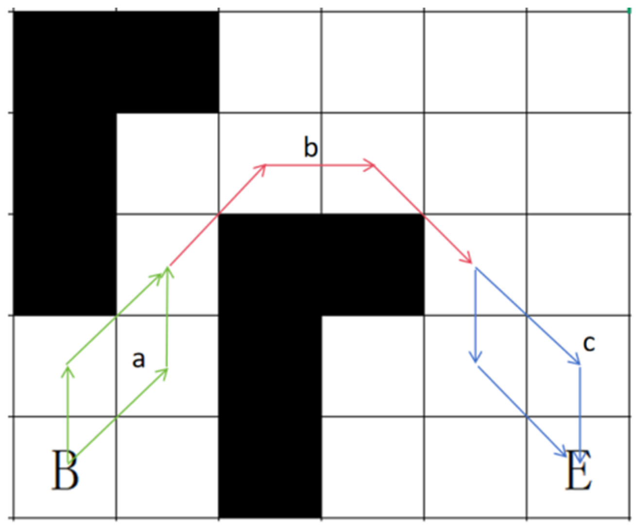
Assuming that in the grid graph  G , under the condition that only eight directions are allowed to move, the shortest path from the starting point B to the end point E requires  m  axial movements and  n  oblique movements, then the relative order of these  m + n  movements can be adjusted arbitrarily without affecting the arrival at the destination. In this paper, these paths are called equivalent paths.
The continuous eight-directional movement path in an obstacle grid can be decomposed into several combinations of equivalent paths. As shown in Figure 6, the continuous eight-directional movement path from grid B to grid E can be divided into three segments. Segments a and c each have two combinations of paths that are equivalent to each other, while segment b can be considered a special equivalent path with one combination of paths.

3.3. Obstacle Vertex Extraction Algorithm (OVEA)

The trajectory of the SGP varies depending on the distribution of obstacles. Directly searching for all obstacle vertices traversed by the SGP is extremely challenging, so it is necessary to break down the SGP. The eight-directional movement can be categorized into two types: movement along the coordinate axes (referred to as axial movement) and movement along the diagonal (referred to as oblique movement). Axial movement does not involve passing through obstacle vertices, whereas diagonal movement might. Therefore, when extracting obstacle vertices, the focus should be on the diagonal movements in the SGP.
We also observed that in the SGP, there are three possible continuous movements: axial–oblique movement, oblique–axial movement, and oblique–oblique movement (axial–axial movement can be optimized at turns, which contradicts the definition of SGP). This implies that in SGPs, at least one of any two consecutive movements is an oblique movement. Based on this observation, we sequentially decompose a complete SGP into these three types of movement combinations and perform obstacle vertex extraction for each pair of consecutive movements.

3.3.1. Axial–Oblique Movement

It is assumed that in an SGP, from grid B to grid M, there are k consecutive axial moves  { m 1 , m 2 , , m k }  and l consecutive oblique moves  { n 1 , n 2 , , n l } , where the starting point of  n i ( i [ 1 , n ] )  is  ( x 1 i , y 1 i ) , and the endpoint is  ( x 2 i , y 2 i ) . For each oblique move, we attempt to translate in the opposite direction of the axial move to construct an equivalent path. We continue until we encounter an obstacle vertex or reach the extension of the previous equivalent path, as illustrated in Figure 7.
Assuming the starting point of  n i  after translation is at the grid  ( x 1 i , y 1 i )  and the endpoint is at the grid  ( x 2 i , y 2 i ) , we will sequentially check the four grids:  ( x 1 i , y 1 i ) ( x 1 i , y 2 i ) ( x 2 i , y 1 i ) , and  ( x 2 i , y 2 i ) . If only one of these four grids is an obstacle, we conclude that  n i  has stopped due to touching an obstacle vertex. If  ( x 1 i , y 1 i )  equals  ( x 2 i 1 , y 2 i 1 ) , we conclude that  n i  has stopped because it has moved to the extension of the previous equivalent path.
After the equivalent path is constructed, for the equivalent path that stops due to touching the obstacle vertex, we add the obstacle vertices it passes in the order of sequence into the TSP candidate point set.

3.3.2. Oblique–Axial Movement

For oblique–axial movement, we can consider it as the reverse of axial–oblique movement. Due to the reversibility of the path, the obstacle vertices encountered during a forward and backward movement along an SGP are the same. Suppose in an SGP, from grid B to grid M, there are k consecutive oblique movements  { m 1 , m 2 , , m k }  and l consecutive axis movements  { n 1 , n 2 , , n l } . By reversing this sequence, the path is transformed into one from grid M to grid B:  { n l , n l 1 , , n 1 , m k , n k 1 , , m 1 } , as shown in Figure 8. The method for axial–oblique movement described in 3.3.1 can then be applied to extract the obstacle vertices encountered and add them to the candidate point set in reverse order.

3.3.3. Oblique–Oblique Movement

For the oblique–oblique movement, we can consider it as a sequence of oblique–axial–oblique movement. The first part of the oblique–axial movement should be reversed according to the strategy outlined in Section 3.3.2 to construct the equivalent path. Since there are no axial movements, the equivalent path for the entire segment is the original path itself. Similarly, the equivalent path for the second part of the axial–oblique movement is also the original path itself, as shown in Figure 9.
Therefore, for oblique–oblique movement, we only need to record the obstacle vertices that pass through it and add them to the candidate points set.
The pseudocode of the obstacle vertex extraction algorithm is shown in Algorithm 1.
Algorithm 1. Obstacle Vertex Extraction Algorithm
Initialize map,  S = { B , s 1 , s 2 , , s n , E } ;
For Every two continuous movement of S in different directions
  Determine the type of two movements;
  IF they are Axial—oblique
    For i = 1 to n
      While  n i  did not touch any obstacles AND  ( x 1 i , y 1 i ) ( x 2 i 1 , y 2 i 1 )
         Move  n i  in the opposite direction along the straight movement;
      END While
      IF There is only one obstacle grid in ( x 1 i , y 1 i ), ( x 1 i , y 2 i ), ( x 2 i , y 1 i ), ( x 2 i , y 2 i )
           IF candidate point set contains ( x 1 i + x 2 i 2 , y 1 i + y 2 i 2 );
             Update the position of ( x 1 i + x 2 i 2 , y 1 i + y 2 i 2 );
         ELSE
           Add ( x 1 i + x 2 i 2 , y 1 i + y 2 i 2 ) to the candidate point set;
         END
      END IF
    END For
  ELSE IF they’re oblique—Axial
    Flip the path;
    Extract obstacle vertices using the Axial—Oblique method;
    Add obstacle vertices in reverse order to the candidate point set;
  ELSE
    Add obstacle vertices to the candidate points set;
  END IF
END For

4. Path-Smoothing Method Based on an Improved Dynamic Programming Algorithm

After extracting all the obstacle vertices that the SGP has passed, not all of these points are included in the TSP. Some points may be non-adjacent but directly connectable, as illustrated in Figure 10c. Therefore, the original problem is transformed into a process of screening the candidate point set, removing points outside the TSP to achieve a smoother path.
Since obstacle vertices are added to the candidate points set by translating and touching obstacles, and these points are added in the order of the SGP, adjacent candidate points can be directly connected. Thus, the points in the candidate point set form a data structure similar to that shown in Figure 11, where all points form a one-way linked list according to their insertion order. Since some path points may be directly connectable, there might be shorter direct connections between some path points.

4.1. Problem Transformation Modeling

It is known that the set of candidate points with length  r + 2  is  P = { B , p 1 , p 2 , , p r , E } . A subsequence  Q = { B , q 1 , q 2 , , q t , E }  was found in  P  with a length  t + 2 ( t r )  such that Formula (5) holds.
L Q = M I N ( L Q 0 ) ,   ( where   Q 0 is   a   subsequence   of   P )
L Q 0 = i = 1 t 1 ( x Q i + 1 x Q i ) 2 + ( y Q i + 1 y Q i ) 2 + ( x Q 1 x B ) 2 + ( y Q 1 y B ) 2 + ( x E x Q t ) 2 + ( y E y Q t ) 2
P and Q should satisfy the following constraints:
q i = p j , ( i [ 1 , r ] , j [ 1 , t ] , i j )
That is,  Q  is a subset of  P .
i = m n 1 S p i , p i + 1 S p m , p n
where  S i , j  represents the straight-line distance between  i  and  j p m , p n P  and  p m , p n  can be directly connected.
That is, the path length of the branch is not greater than that of the main chain.

4.2. Improved Dynamic Programming Algorithm

Lemma 1.
If  P = { v 1 , v 2 , , v k }  is the shortest path from  v 1  to  v k , then for any two nodes  v i  and  v j   ( 1 i j k )  in this path, the sub-path  P i j = { v i , v i + 1 , , v j }  is also the shortest path from  v i  to  v j .
The following proves the feasibility of using dynamic programming algorithm for this problem.
Proof. 
Since  Q  is a TSP from  B  to  E Lemma 1 indicates that  Q  has the property of optimal substructure. If there is a common point  p j = q i  in  P Q , and  p j P Q , then the subsequence  { B , q 1 , q 2 , , q i }  of  Q  forms a TSP from  B  to  q i , and the subsequence  { q i , q i + 1 , , q t , E }  of  Q  forms a TSP from  q i  to  E . According to the definitions of  P  and  Q { B , q 1 , q 2 , , q i }  is a subsequence of  { B , p 1 , p 2 , , p j } , and  { q i , q i + 1 , , q t , E }  is a subsequence of  { p j , p j + 1 , , p r , E } . This means that the optimal solution to this problem can be broken down into the optimal solutions of these subproblems. Therefore, this problem also possesses the property of optimal substructure, and it can be solved using dynamic programming algorithms. □
Since this problem not only requires obtaining the path length but also storing the shortest path, an additional array is needed during the dynamic programming process to record the historical optimal paths. However, as the algorithm runs, the number of nodes in the historical optimal paths increases, causing the array’s length to vary, which is not conducive to pre-allocating space. Moreover, when the problem scale is large, a significant amount of storage space is required for these paths. To address this issue, we leverage the characteristic of the optimal substructure of candidate point sets by setting up an auxiliary array that stores the indices of predecessor nodes instead of the paths themselves, as shown in Figure 12.
It is also noted that the set of candidate points has the following properties:
Property 1.
The subsequent adjacent points of a point in the candidate set extracted by SGPs are continuous in the candidate set.
Proof of Property 1.
Suppose that in the candidate set of a certain SGP, the subsequent adjacent points of a point are discontinuous in the set. That is, there exists a continuous subsequence  { A , , B , C , , D } , where  { A , , B }  are adjacent points, A and C are not adjacent, D is a subsequent candidate point of C, and A and D are adjacent.
Since  A  and  C  are not adjacent points, the line connecting  A  and  C  must pass through an obstacle or a common vertex of two obstacle grids. Connect point A to the boundary point of the obstacle to form two lines a and b, as shown in Figure 13. Since  A  and  D  are adjacent,  D  must be located outside lines a and b. If  D  is on the outside of line a, because  A  and  D  are adjacent, line  A D  will not pass through the obstacle or the wall gap (which is considered illegal in this context). This means there is a shorter SGP between  A D  that does not need to bypass the obstacle between  A C , which contradicts the definition that the SGP should be the shortest eight-directional movement path. Similarly, if  D  is on the outside of line b, there is also a shorter SGP, leading to another contradiction. Therefore,  A  and  D  are not adjacent points, and Property 1 holds. □
From Property 1, we can deduce the following.
Inference 1.
For any two nodes  p i  and  p j ( 1 i j r )  in the candidate point set  P = { B ,   p 1 , p 2 , , p r , E } , where the set of pre-adjacent points of  p i  is  p i u { p u , p u + 1 , , p i 1 }  and the set of pre-adjacent points of  p j  is  p j v { p v , p v + 1 , , p j 1 } , if  i < j , then  u v .
Proof of Inference 1.
Assume  i < j  and  u > v  According to Property 1, the set of adjacent points after  p u  is  { p u + 1 , p u + 2 , , p k } ( k i ) , and the set of adjacent points after  p v  is { p v + 1 , p v + 2 , p l }(l ≥ j). Since  l j  and  i < j , it follows that  l > i , so  p v  and  p i  are adjacent points. Furthermore, since  u > v p i u { P v , P v + 1 , , P i 1 } , which contradicts  p i u { P u , P u + 1 , , P i 1 } . Therefore, Inference 1 holds. □
Inference 1 indicates that the boundary of the set of preceding adjacent points for a path point will shift backward as the point moves through the candidate point set. Therefore, a sliding window can be used to optimize dynamic programming algorithms, thereby enhancing their efficiency. The sliding window defines the range of the preceding adjacent points and gradually advances toward the endpoint during the loop.
The flow chart of the optimized dynamic programming algorithm is shown in Figure 14.

5. Experiment

5.1. Experimental Environment

All experiments in this paper were conducted using MATLAB R2023a software on a computer equipped with 16 GB of RAM and a 2.20 GHz processor. Except for the test of the benchmark data set, all maps used in the experiments were randomly generated by the system according to the input map side length N, and the obstacle grid was randomly selected according to the input obstacle rate ρ. The horizontal and vertical coordinates of the starting point and the end point were generated by taking random positive integers within the range of 0 to N.

5.2. Ablation Experiment

To evaluate the effectiveness and importance of each component of SGPVEFA, this paper conducts ablation experiments by removing various steps of the algorithm to assess their impact on the overall algorithm. The test subjects include the basic algorithm (Basic), which only performs SGP search without optimization; the obstacle vertex extraction algorithm (OVEA), which removes the obstacle extraction module from the overall algorithm; the path-smoothing method (PSM), which removes the path-smoothing module from the overall algorithm; and the SGP vertex extraction filtering algorithm (SGPVEFA).
The experiment randomly generates 100 maps, with the map side length N increasing from 100 to 1000, with each increment of 100. For each N, 10 maps are randomly generated, and for each map, a random obstacle grid and start/finish points are created, with an obstacle rate of 0.3. The changes in path length for each sub-algorithm as the map side length N increases are shown in Figure 15, and the changes in search time as the map side length N increases are shown in Figure 16. Since the search time approaches zero when the map side length is too small, Figure 16 only shows part of the search time for  N 400 .
From Figure 15, it is evident that if obstacle vertices are not extracted and path smoothing is performed directly, the total path length can be reduced to a certain extent, but it cannot be optimized. If only obstacle vertices are extracted without path smoothing, the total path length might even slightly increase. This is because the set of obstacle vertices includes irrelevant points, which may cause unnecessary turns. Only by running both parts simultaneously can the path length be optimized. As shown in Figure 16, the time consumed by SGPVEFA is minimal, and almost negligible compared to the search time for SGPs.
The ablation experiment shows that SGPVEFA is very efficient and can further shorten SGPs in a short space of time, and the optimization effect is more significant with the increase in map size.

5.3. Testing on the Benchmark Data Set

To evaluate the performance of SGPVEFA in practical applications, we applied it to real-world data sets. The data set used for testing was sourced from the 2D grid world benchmarks at Nathan Sturtevant’s Mobile AI Lab (See the data availability statement at the end of this article). This data set includes street images from major cities such as Berlin, Boston, and London, with three resolutions:  256 × 256 512 × 512 , and  1024 × 1024 . We selected 10 real-world maps from each resolution for testing, with the starting and ending points set at the top-left and bottom-right corners of the map, respectively. Figure 17 shows some of the paths found by SGPVEFA, and Table 1 provides the average path lengths found at different resolutions (rounded to two decimal places).
It should be noted that the path shown in Figure 17 seems to have some unnecessary turns, which is caused by the resolution. Some discrete obstacle grids are difficult to display on a large-scale grid map.
The test results show that the path searched by SGPVEFA is consistent with TSP, and the overall path is very smooth with very few path points, which greatly reduces the number of turns in actual path planning. SGPVEFA can complete the task well under different resolutions.

5.4. Comparison Experiment of Intelligent Path Planning Algorithms

In order to test the performance of SGPVEFA compared with intelligent path planning algorithms, we set up a comparative experiment with intelligent path planning algorithms (GA, GWO [22], DE [23], PSO, SSA [24], etc.). We will conduct comparative experiments considering two aspects: map size and obstacle rate.

5.4.1. Map Size

In the experiment, seven sets of grid maps were randomly generated, and the side length N of the map was increased from 100 to 700 with an increment of 100 each time. The obstacle grid and starting point were randomly generated on each map (ensuring feasible solutions), and the obstacle rate ρ was set to 0.1.
The parameters for each algorithm are set as follows: the maximum number of iterations is 100, and the population size is 50. The crossover probability (pc) in Genetic Algorithm (GA) is 0.8, and the mutation probability (pm) is 0.05. In the GWO algorithm, the initial value of the control parameter a is 2, which decreases to 0 with each iteration. For the DE algorithm, the mutation probability f is a random number between  [ 0.2 , 0.8 ] , and the crossover probability  c r  is 0.2. In the PSO algorithm, the inertia weight ω is 0.8, the individual learning factor  c 1  is 1.2, and the group learning factor  c 2  is 1.2. The SSA algorithm has an explorer ratio  P p e r c e n t  of 0.2.
The path length of each algorithm changes with the map edge length N as shown in Figure 18, and the search time changes with the map edge length N as shown in Figure 19. Since the search time approaches 0 when the map edge length is too small, only part of the search time comparison is given in Figure 19.
The experiments show that SGPVEFA has a clear advantage in terms of path length, and this advantage becomes more pronounced as N increases. In terms of search time, when N is small, SGPVEFA’s search time is slightly shorter than that of the intelligent path planning algorithm. As N increases, SGPVEFA’s search time aligns with that of the intelligent path planning algorithm (excluding GA).

5.4.2. Obstacle Rate

When there are many obstacles, the intelligent optimization algorithm may fail to find a feasible solution. Therefore, we conducted comparative experiments on the success rate and solution quality of each algorithm under three different obstacle rates. The success of an algorithm is marked by successful population initialization and finding a feasible solution within the specified number of iterations. The experiment involved randomly generating three sets of grid maps, with 50 maps in each set. Each map has a side length of 500 × 500, and the obstacle rate  ρ  was set to 0.1, 0.2, and 0.3, respectively. Obstacle grids and start/finish points were randomly generated on each map (ensuring there is a feasible solution). The parameter settings for each algorithm are the same as in Section 5.4.1. The success rate test results for each algorithm are shown in Table 2. In cases where the algorithms succeeded, the comparison of path lengths, search times, and SGPVEFA is presented in Table 3.
As shown in Table 2, the proposed algorithm can still accurately find feasible solutions for complex maps. However, as the obstacle rate increases, the success rate of the intelligent optimization algorithm drops significantly. When the obstacle rate reaches 0.3, the success rate is below 10%, and for Genetic Algorithm (GA), it is only 2%, making it almost impossible to find a solution. This highlights the superiority of SGPVEFA in high-obstacle environments. In Table 3, as the obstacle rate increases, the search time and path length of each algorithm decrease. This is because the starting and ending points are randomly generated, and the intelligent optimization algorithm can only handle short-distance problems under high obstacle conditions. For longer distances between the starting and ending points, no feasible solution can be found. In short-distance scenarios, both the path length and search time are reduced.
It can be seen that in the three obstacle rate environments, SGPVEFA’s search time and path length are better than those of intelligent optimization algorithm.

5.5. Comparative Experiments of New Algorithms in Recent Years

We also conducted comparative experiments with some path planning algorithms proposed in recent years, such as the improved artificial bee algorithm (IABC) proposed in [25] and the improved butterfly optimization algorithm (IBOA) proposed in [26].

5.5.1. Compared with IABC

We tested SGPVEFA using the same environment maps from [25], comparing the results with those from [25]. The IABC parameters were set as follows: 200 maximum iterations, 50 initial population size, and 100 maximum population size. The four environments were configured as follows: a simple environment with regular obstacles (Environment 1, obstacle rate 0.19), a complex environment with regular obstacles (Environment 2, obstacle rate 0.26), a simple environment with random obstacles (Environment 3, obstacle rate 0.17), and a complex environment with random obstacles (Environment 4, obstacle rate 0.22). The paths found by the two algorithms in different environments are shown in Figure 20. Table 4 provides the mean path lengths and node counts, along with the optimal values and standard deviations for both algorithms. SGPVEFA is an exact algorithm, and its results are consistent across all runs.
In the comparative experiment of Environment 4, the optimal path found by IABC slightly outperformed the algorithm proposed in this paper. This is because in Environment 4, IABC frequently encountered paths that crossed through the common point of two obstacle grids, a scenario that the proposed algorithm in this paper avoids for safety reasons (It has been stated in Section 2). Under the same conditions, SGPVEFA still outperforms IABC.
Experiments show that, whether in simple or complex obstacle environments, the paths found by SGPVEFA are smoother compared to those found by IABC, with fewer turns and nodes, and shorter path lengths. In complex obstacle environments, IABC often encounters walls, whereas SGPVEFA avoids such issues, making it safer in real-world applications.

5.5.2. Compared with IBOA

We tested SGPVEFA using the same environment maps from [26], comparing the results with those from [26]. The IBOA parameters were set as follows: a maximum of 50 iterations, a population size of 4000, and the two path simplification strategies proposed in [26]. On a complex obstacle map of 40 × 40, the paths found by the two algorithms are illustrated in Figure 21, and the path lengths and node counts are listed in Table 5.
Experiments show that SGPVEFA still has advantages over IBOA with the combined path simplification strategy in terms of path length and number of path nodes, which makes the path searched by SGPVEFA smoother and with fewer turns.

6. Conclusions

This paper introduces an SGP vertex extraction filtering algorithm designed to optimize the SGP in obstacle grid maps into the TSP. This algorithm can find a shorter and smoother route than intelligent path planning algorithms within a short time frame. In scenarios involving large-scale maps and high obstacle densities, the performance of SGPVEFA is particularly outstanding.
From the ablation experiments in Section 5.2 of the paper, it is evident that SGPVEFA spends very little time optimizing an SGP into a TSP, with most of its time dedicated to solving the SGP problem. The algorithm’s complexity is determined by the number of points in the given SGP and the distribution of obstacles, rather than the map’s dimensions. Therefore, increasing the map size does not degrade the algorithm’s efficiency, but it does slow down the search for SGPs. However, due to the low coupling degree of SGPVEFA, when dealing with larger problem scales, we can integrate it with heuristic algorithms. First, we used heuristic algorithms to solve SGPs, and then applied this algorithm to solve TSPs.
However, due to the complexity of two-dimensional obstacle grid maps, this paper has not yet provided rigorous proof that this method can solve the TSP. Additionally, SGPVEFA has certain limitations. For example, SGPVEFA requires pre-acquiring the SGP of the obstacle grid map, whereas some heuristic algorithms do not require this step, which may limit its applicability. Moreover, it can only solve problems with obstacle grid maps, and in real-world scenarios, the problem needs to be modeled into a similar situation, which is not an easy task. Furthermore, SGPVEFA is a static algorithm, and obstacles and feasible paths can change over time, necessitating the integration of dynamic response mechanisms. Additionally, the problems we encounter are not limited to two-dimensional planes; for instance, in drone path planning, future research could explore extending SGPVEFA to three-dimensional space. In recent years, many new heuristic techniques have been developed to optimize complex nonlinear problems, such as the Beetle Antennae Olfactory Recurrent Neural Network [27] and BAS-ADAM [28]. We will attempt to compare or integrate these new technologies in our future research.

Author Contributions

Conceptualization, Y.Z.; methodology, Y.Z.; software, J.C.; validation, Y.Z. and J.C.; formal analysis, Y.Z.; investigation, J.C.; resources, J.C.; data curation, J.C.; writing—original draft preparation, J.C.; writing—review and editing, Y.Z.; visualization, J.C.; supervision, Y.Z.; project administration, Y.Z.; funding acquisition, Y.Z. All authors have read and agreed to the published version of the manuscript.

Funding

This study was funded by National Natural Science Foundation of China (Grant No.: 62402200).

Institutional Review Board Statement

Not applicable.

Informed Consent Statement

Not applicable.

Data Availability Statement

The benchmark data set used in Section 5.3 of this paper is from the following link. https://www.movingai.com/benchmarks/street/index.html. Accessed on 20 June 2025. The rest of the data are randomly generated.

Conflicts of Interest

This study does not have any conflicts of interest with any organization or individual.

References

  1. Braekers, K.; Ramaekers, K.; Van Nieuwenhuyse, I. The vehicle routing problem: State of the art classification and review. Comput. Ind. Eng. 2016, 99, 300–313. [Google Scholar] [CrossRef]
  2. Pop, P.C.; Cosma, O.; Sabo, C.; Sitar, C.P. A comprehensive survey on the generalized traveling salesman problem. Eur. J. Oper. Res. 2024, 314, 819–835. [Google Scholar] [CrossRef]
  3. Davoodi, M.; Panahi, F.; Mohades, A.; Hashemi, S.N. Clear and smooth path planning. Appl. Soft Comput. 2015, 32, 568–579. [Google Scholar] [CrossRef]
  4. Dijkstra, E.W. A note on two problems in connexion with graphs. In Edsger Wybe Dijkstra: His Life, Work, and Legacy; Association for Computing Machinery: New York, NY, USA, 2022; pp. 287–290. [Google Scholar]
  5. Holland, J.H. Genetic algorithms. Sci. Am. 1992, 267, 66–73. [Google Scholar] [CrossRef]
  6. Alberto, C.; Dorigo, M.; Maniezzo, V. An Investigation of some Properties of an “Ant Algorithm”. PPSN 1992, 92, 509–520. [Google Scholar]
  7. Kennedy, J.; Eberhart, R. Particle swarm optimization. In Proceedings of the ICNN’95—International Conference on Neural Networks, Perth, WA, Australia, 27 November–1 December 1995; Volume 4, pp. 1942–1948. [Google Scholar] [CrossRef]
  8. Katona, K.; Neamah, H.A.; Korondi, P. Obstacle Avoidance and Path Planning Methods for Autonomous Navigation of Mobile Robot. Sensors 2024, 24, 3573. [Google Scholar] [CrossRef]
  9. Hussain, K.; Salleh, M.N.M.; Cheng, S.; Shi, Y. Metaheuristic research: A comprehensive survey. Artif. Intell. Rev. 2019, 52, 2191–2233. [Google Scholar] [CrossRef]
  10. Reeves, C. Landscapes, operators and heuristic search. Ann. Oper. Res. 1999, 86, 473–490. [Google Scholar] [CrossRef]
  11. Yahia, H.S.; Mohammed, A.S. Path planning optimization in unmanned aerial vehicles using meta-heuristic algorithms: A systematic review. Environ. Monit. Assess. 2023, 195, 30. [Google Scholar] [CrossRef]
  12. Wu, H.; Cheng, J.; Ke, Y.; Huang, S.; Huang, Y.; Wu, H. Efficient Algorithms for Temporal Path Computation. IEEE Trans. Knowl. Data Eng. 2016, 28, 2927–2942. [Google Scholar] [CrossRef]
  13. Liu, H.; Jin, C.; Yang, B.; Zhou, A. Finding Top-k Shortest Paths with Diversity. IEEE Trans. Knowl. Data Eng. 2018, 30, 488–502. [Google Scholar] [CrossRef]
  14. Cosma, O.; Pop, P.C.; Zelina, I. An Effective Genetic Algorithm for Solving the Clustered Shortest-Path Tree Problem. IEEE Access 2021, 9, 15570–15591. [Google Scholar] [CrossRef]
  15. Ramamoorthy, R. An improved distance-based ant colony optimization routing for vehicular ad hoc networks. Int. J. Commun. Syst. 2020, 33, e4502. [Google Scholar] [CrossRef]
  16. Bailey, J.P.; Nash, A.; Tovey, C.A.; Sven, K. Path-length analysis for grid-based path planning. Artif. Intell. 2021, 301, 103560. [Google Scholar] [CrossRef]
  17. Hew, P.C. The length of shortest vertex paths in binary occupancy grids compared to shortest r-constrained ones. J. Artif. Intell. Res. 2017, 59, 543–563. [Google Scholar] [CrossRef]
  18. Alex, N.; Koenig, S. Any-angle path planning. AI Mag. 2013, 34, 85–107. [Google Scholar]
  19. Daniel, H.; Grastien, A. An optimal any-angle pathfinding algorithm. In Proceedings of the International Conference on Automated Planning and Scheduling, Rome, Italy, 10–14 June 2013; Volume 23. [Google Scholar]
  20. Yap, P.; Burch, N.; Holte, R.C.; Schaeffer, J. Any-angle path planning for computer games. In Proceedings of the AAAI Conference on Artificial Intelligence and Interactive Digital Entertainment, Palo Alto, CA, USA, 10–14 October 2011; Volume 7. [Google Scholar]
  21. Roy, M.; Foufou, S.; Koschan, A.; Truchetet, F.; Abidi, M. Multiresolution analysis for irregular meshes. In Wavelet Applications in Industrial Processing; SPIE: Bellingham, WA, USA, 2004; Volume 5266. [Google Scholar]
  22. Mirjalili, S.; Mirjalili, S.M.; Lewis, A. Grey wolf optimizer. Adv. Eng. Softw. 2014, 69, 46–61. [Google Scholar] [CrossRef]
  23. Storn, R.; Price, K. Differential Evolution—A Simple and Efficient Heuristic for global Optimization over Continuous Spaces. J. Glob. Optim. 1997, 11, 341–359. [Google Scholar] [CrossRef]
  24. Xue, J.; Shen, B. A novel swarm intelligence optimization approach: Sparrow search algorithm. Syst. Sci. Control. Eng. 2020, 8, 22–34. [Google Scholar] [CrossRef]
  25. Yildirim, M.Y.; Akay, R. An efficient grid-based path planning approach using improved artificial bee colony algorithm. Knowl.-Based Syst. 2025, 318, 113528. [Google Scholar] [CrossRef]
  26. Zhai, R.; Xiao, P.; Shu, D.; Sun, Y.; Jiang, M. Application of improved butterfly optimization algorithm in mobile robot path planning. Electronics 2023, 12, 3424. [Google Scholar] [CrossRef]
  27. Khan, A.H.; Li, S.; Luo, X. Obstacle avoidance and tracking control of redundant robotic manipulator: An RNN-based metaheuristic approach. IEEE Trans. Ind. Inform. 2019, 16, 4670–4680. [Google Scholar] [CrossRef]
  28. Khan, A.H.; Cao, X.; Li, S.; Katsikis, V.N.; Liao, L. BAS-ADAM: An ADAM based approach to improve the performance of beetle antennae search optimizer. IEEE/CAA J. Autom. Sin. 2020, 7, 461–471. [Google Scholar] [CrossRef]
Figure 1. Obstacles covered with a grid map.
Algorithms 18 00400 g001
Figure 2. Better fitting obstacles by increasing the resolution of the grid.
Algorithms 18 00400 g002
Figure 3. SGP and TSP (Where B is the starting point and E is the end point).
Algorithms 18 00400 g003
Figure 4. A TSP is a series of lines connecting obstacle vertices (Where B is the starting point and E is the end point).
Algorithms 18 00400 g004
Figure 5. Flow chart of SGPVEFA.
Algorithms 18 00400 g005
Figure 6. The 8-direction path can be divided into several equivalent path combinations.
Algorithms 18 00400 g006
Figure 7. Axial–oblique movement to construct equivalent paths and search obstacle vertices.
Algorithms 18 00400 g007
Figure 8. Oblique–axial movement is reversed to axial–oblique movement (where the blue line represents oblique–axial movement and the red line represents axial–oblique movement).
Algorithms 18 00400 g008
Figure 9. Oblique–oblique movement directly records the obstacle vertex passed.
Algorithms 18 00400 g009
Figure 10. An example of path-smoothing algorithm.
Algorithms 18 00400 g010
Figure 11. Data structure for a set of candidate points of length n (ellipses represent path points and numbers represent their order in the set, and arrows indicate that there is a path in the set).
Algorithms 18 00400 g011
Figure 12. Replace the path array with an index array.
Algorithms 18 00400 g012
Figure 13. The adjacent points of the points in the candidate set are continuous in the set.
Algorithms 18 00400 g013
Figure 14. Improved dynamic programming algorithm flow chart.
Algorithms 18 00400 g014
Figure 15. Comparison of path lengths in each part of the ablation experiment.
Algorithms 18 00400 g015
Figure 16. Comparison of search time for each part of ablation experiment.
Algorithms 18 00400 g016
Figure 17. Some test results of SGPVEFA on the actual data set.
Algorithms 18 00400 g017
Figure 18. Comparison experiment of intelligent path planning algorithms (path length).
Algorithms 18 00400 g018
Figure 19. Comparison experiment of intelligent path planning algorithms (search time).
Algorithms 18 00400 g019
Figure 20. Path comparison under different environments.
Algorithms 18 00400 g020
Figure 21. Comparison of paths found in complex environments.
Algorithms 18 00400 g021
Table 1. The average path length searched by SGPVEFA is compared with the TSP.
ResolutionSGPVEFATSP
256 × 256363.46363.46
512 × 512755.91755.91
1024 × 10241534.811534.81
Table 2. Success rate of each algorithm.
AlgorithmSGPVEFAGAGWODEPSOSSA
Obstacle rateNumber of runs505050505050
0.1success501432323231
success rate100%28%64%64%64%62%
0.2success50719191919
success rate100%14%38%38%38%38%
0.3success5014444
success rate100%2%8%8%8%8%
Table 3. Comparison of path length and search time with GA.
Obstacle RateAlgorithmSGPVEFAGAGWODEPSOSSA
0.1path length161.41644.6654.27929.55791.47281.26
search time4.066.8413.8513.7513.4913.74
0.2path length185.4485.63460.11584.79541.41257.25
search time4.6226.4525.6425.042727.31
0.3path length93.26186.4124.99168.09119.89102.09
search time0.784.792.121.861.531.77
Table 4. Comparison of path length and number of nodes with IABC.
EnvironmentAlgorithmPath LengthNumber of Nodes
1SGPVEFA40.0766
IABCBestMeanStd.BestMeanStd.
41.24541.245011110
2SGPVEFA52.9210
IABCBestMeanStd.BestMeanStd.
55.63955.7140.32461818.9330.2537
3SGPVEFA27.0245
IABCBestMeanStd.BestMeanStd.
27.46228.7950.9889810.41.6316
4SGPVEFA28.7249
IABCBestMeanStd.BestMeanStd.
28.50129.6140.47331215.0331.2726
Table 5. Comparison of path length and number of nodes with IBOA.
AlgorithmPath LengthNumber of Nodes
SGPVEFA58.28910
IBOA61.01619
Disclaimer/Publisher’s Note: The statements, opinions and data contained in all publications are solely those of the individual author(s) and contributor(s) and not of MDPI and/or the editor(s). MDPI and/or the editor(s) disclaim responsibility for any injury to people or property resulting from any ideas, methods, instructions or products referred to in the content.

