Abstract
Rank aggregation deals with the problem of fusing multiple ranked lists of elements into a single aggregate list with improved element ordering. Such cases are frequently encountered in numerous applications across a variety of areas, including bioinformatics, machine learning, statistics, information retrieval, and so on. The weighted rank aggregation methods consider a more advanced version of the problem by assuming that the input lists are not of equal importance. In this context, they first apply ad hoc techniques to assign weights to the input lists, and then, they study how to integrate these weights into the scores of the individual list elements. In this paper, we adopt the idea of exploiting the list weights not only during the computation of the element scores, but also to determine which elements will be included in the consensus aggregate list. More specifically, we introduce and analyze a novel refinement mechanism, called WIRE, that effectively removes the weakest elements from the less important input lists, thus improving the quality of the output ranking. We experimentally demonstrate the effectiveness of our method in multiple datasets by comparing it with a collection of state-of-the-art weighted and non-weighted techniques.
1. Introduction
Rank aggregation algorithms accept as input a set of ordered element lists submitted by a group of rankers. Then, they process these lists and return a consensus ranking with enhanced element ordering. Such problems are quite common in numerous research fields, such as bioinformatics [1,2], sports [3], recommendation systems [4,5], information retrieval [6,7,8], ballots [9,10], and so forth.
Most existing methods consider that input lists are of equal importance. Hence, they do not investigate issues where, for example, a list is submitted by an expert or a non-expert ranker, or a spammer submits a preference list in order to promote or downgrade specific elements. Although this non-weighted approach aligns with several application areas (e.g., fair elections), in other cases, such as collaborative filtering systems, it usually leads to output lists that suffer from bias, manipulation, and low-quality element ranking.
In contrast, the weighted rank aggregation methods take the aforementioned issues into account and attempt to assess the input list quality before they fuse them into a single ranking [11,12,13]. By applying unsupervised exploratory analysis techniques, they assign weights to the input lists with the aim of evaluating their significance. In the sequel, they exploit these weights during the computation of the scores of the respective list elements. More specifically, the list weights are embodied in the individual element scores, thus affecting their ranking in the output list.
In the vast majority of cases, this is how the weighted methods exploit the learned list weights. However, the distance-based method of Akritidis et al. [13] introduced a more inspiring approach. First, an iterative algorithm was applied to estimate the importance of the input lists by measuring their distances from the generated output list. Then, the distance-based ranker weights were used in two ways as follows: (i) to compute the element scores in a manner that promotes those submitted by expert rankers, and (ii) to prevent low-quality elements submitted by non-expert rankers from entering the final aggregate list. In this context, the learned weights were used to determine the number of elements that each input list contributed to the final ranking.
The experiments of [13] demonstrated that weight-based list pruning can yield promising results, especially when the input lists are long. However, for input lists that consist of only a few items, the gains are considerably limited, or even reversed in some cases. These findings indicate that a more sophisticated approach is required to fully exploit the learned ranker weights.
To alleviate this issue, this paper introduces a novel, unsupervised method, called WIRE, that regulates the contribution of each input list in the formulation of the aggregate list. In contrast to the suggestions of [13], our strategy does not simply remove elements from the bottom of the input lists, but it carefully removes the weakest elements, with respect to their overall score, from the less important lists, with respect to their weights. In this way, it constructs aggregate lists of improved quality, even when the input preference lists are short. In addition, note that this refinement mechanism depends only on the input lists, the consensus ranking, and the weights of the involved rankers. Since this information is directly accessible either from the input or from the base aggregator, two major advantages of WIRE are derived. First, it fits into any weighted rank aggregation method and can be applied as a post-processing step. Second, its independence from individual element or list attributes (e.g., ranks, scores, lengths, etc.) renders it capable of handling partial rankings. These design choices increase our method’s flexibility and applicability.
The remainder of this paper is organized as follows. Section 2 provides a brief overview of the relevant literature on weighted rank aggregation. Several preliminary elements are discussed in Section 3, whereas the proposed weighted item selection algorithm is presented and analyzed in Section 4. Section 5 describes the experimental evaluation and discusses the acquired results. The paper is concluded in Section 6 with the most significant findings and points for future research.
2. Related Work
The need for designing fair elections is quite old and has attracted the attention of researchers many decades ago. The Borda Count [14] and Condorcet criterion [15] are among the oldest rank aggregation methods that have been introduced for this purpose. Nowadays, rank aggregation has numerous applications in a wide variety of research areas, including information retrieval, bioinformatics, ballots, etc. [16,17,18].
In [19], Dwork et al. introduced four rank aggregation methods based on Markov chains to combine rankings coming from different search engines. Originally proposed to combat spam entries, the four methods are derived by considering different forms of the chain’s transition matrix. Similarly, Ref. [20] adopted a Markov chain framework to compare the results of multiple microarray experiments expressed as ranked lists of genes.
The robust rank aggregation method of [21] proposed an unbiased probabilistic technique to process the results of various genomic analysis applications. More specifically, it compared the actual ranking of an element with the ranking provided by a null model that dictated random ordering. This strategy renders it robust to outliers, noise, and errors.
On the other hand, the order-based methods examine the relevant rankings of the items in the input lists, assigning them scores based on their pairwise wins, ties, and losses. The Condorcet method was among the first approaches to adopt this logic [15]. Similarly, the well-known Kemeny–Young method is based on a matrix that also counts the pairwise preferences of the rankers [22,23]. Then, it uses this matrix to assign scores to each possible permutation of the input elements. Its high computational complexity—the problem is NP-Hard even for four rankers—rendered it inappropriate for datasets having many input lists. More recently, the outranking approach of [24] introduced four threshold values to quantify the concordance or discordance between the input lists.
The aforementioned methods have been proven to be quite effective in a variety of tasks. However, they do not take into consideration the level of expertise of the rankers who submit their preference lists. Consequently, they are prone to cases where a ranker may attempt to manipulate the output ranking by submitting spam entries, or simply, to rankers with different importance degrees.
The work of Pihur et al. proposed a solution that optimized the weighted distances among the input lists [25]. Based on the traditional Footrule distance, the authors established a function that combined the list weights with the individual scores that were assigned to each element by its respective rankers. However, in many cases, these scores are unknown (that is, they are not included in the input lists); therefore, the distance computation is rendered intractable.
The weighted method of Desarkar et al. modeled the problem by constructing preference relation graphs [26]. The list weights were subsequently computed by verifying the validity of several custom majoritarian rules. Furthermore, Chatterjee et al. introduced another weighted technique for crowd opinion analysis applications by adopting the principles of agglomerative clustering [27].
More recently, an iterative distance-based method called DIBRA was published in [13]. At each iteration, DIBRA computes the distances of the input lists from an aggregate list that is derived by applying a simple baseline method like the Borda Count. The lists that are proximal to the aggregate list are assigned higher weights, compared to the most distant ones. This process is repeated until all weights converge and the aggregate list is stabilized. Interestingly, Ref. [13] also introduced the idea of exploiting the learned weights to limit the contribution of the weakest rankers in the formulation of the aggregate list. In particular, the number of elements that participate in the aggregation process is determined by the weight of the respective preference list.
This simple pruning mechanism has been proven to be beneficial in several experiments that involved long input lists. However, for shorter lists, the gains were either minimized or reversed. This study introduces an item selection method that performs significantly better in all cases.
3. Weighted Rank Aggregation
A typical rank aggregation scenario involves a group of n rankers that submits n preference lists and an aggregation algorithm that combines these preference lists with the aim of finding a consensus ranking . In this paper, we consider the most generic version of the problem, where the preference lists (i) can be of variable length and (ii) may include only a subset of the entire universe S of the elements; such lists are called partial. In contrast, full lists contain permutations of all elements of S, so they are of equal lengths.
A typical non-weighted aggregator receives the preference lists as input and assigns a score value to each element i, according to its ranking in the input lists, the number of pairwise wins and losses, or other criteria. Then, it outputs the unique elements of the lists sorted in score order, thus producing a consensus ranked list as follows:
In contrast, a weighted aggregator employs an unsupervised mechanism that evaluates the importance of each ranker u, by taking into account its preferences and several other properties. In the sequel, it integrates these weights in the computation of the element scores as follows:
In [13], the authors also introduced a post-processing technique that removes the low-ranked elements from each input list based on the weights of their respective rankers as follows:
In this study, we propose a new list pruning mechanism with the aim of improving the quality of the aggregate list . The block diagram of Figure 1 illustrates the sequential flow of the aforementioned procedure.
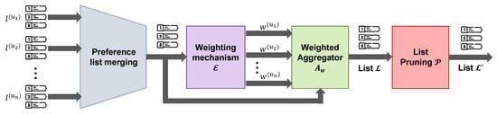
Figure 1.
Schematic diagram of weighted rank aggregation with list pruning.
4. WIRE: Algorithm Design and Analysis
Algorithm description. Most weighted rank aggregation methods integrate the learned weights into the scores of the individual elements, with the sole objective of improving the quality of their produced ranking. As mentioned earlier, a representative exception is the list pruning policy of [13], which uses the learned ranker weights to remove the weakest elements from the input lists. In the sequel, we introduce a new method called WIRE (Weighted Item Removal) that utilizes the learned list weights to effectively determine the contribution of each input preference list in the formulation of the output list .
WIRE introduces a novel mechanism that identifies appropriate list elements for removal. Notably, this mechanism depends only on the input preference lists, the ranker weights, and the consensus ranking. This increases the flexibility of our algorithm, since its independence from other factors (e.g., the scores of the input list elements) enables its attachment to any weighted rank aggregation method as a post-processing step.
On the other hand, if cannot estimate the ranker weights in a robust manner, then the ability of WIRE to identify the weakest elements will inevitably decrease. For this reason, we present WIRE in the context of DIBRA, the distance-based weighted method that was introduced in [13]. The experiments of [13] have shown that DIBRA is superior to other weighted algorithms (e.g., [26,27]), and this was also verified in the present experiments. Therefore, even though our method can be applied in combination with any weighted rank aggregation method, the capability of DIBRA in distinguishing the expert rankers from the non-experts renders it a suitable basis for applying WIRE.
In short, DIBRA capitalizes on the concept that the importance of a ranker is determined by the distance of its preference list from the consensus ranking . In this spirit, it iteratively adjusts the weight of a ranker u by using the following equation:
where and are the weight of ranker u and the aggregate list after i iterations, respectively. Moreover, d represents a function that quantifies the distance between the preference list and the aggregate list . The form of Equation (5) guarantees that the weights converge after several iterations, usually between 5 and 20.
After the voter weights have been calculated and the final aggregate list has been constructed, WIRE is deployed to further improve the quality of . The proposed method refines the input preference lists by removing their weakest elements and operates in five phases, according to Algorithm 1.
| Algorithm 1 WIRE: Weighted Item Removal |
Input: Rankers , Ranker weights , Preference lists , number of buckets , hyper-parameter Output: Aggregate list .
|
Initially, the rankers are sorted in decreasing weight order. Then, they are distributed into a set of equally sized buckets in such a manner that each bucket contains rankers. Since the ranker weights are sorted in descending order, the first bucket will contain the expert rankers, that is, those who received the highest weights; the second bucket will include the rankers with lower weights, and so on. We now introduce an exponentially decaying confidence score for each bucket as follows:
where is a hyper-parameter that specifies the minimum confidence score of a bucket. The confidence scores of Equation (6) are inherited by all rankers belonging to a particular bucket, as shown in step 11 of Algorithm 1. Therefore, the rankers of the first bucket () receive a confidence score , regardless of the total number of buckets B. Similarly, all rankers in the second bucket () are assigned a confidence score , etc. Notice that .
Subsequently, for each element we introduce the following preservation score:
where denotes the bucket in which the ranker u has been placed. Equation (7) indicates that the preservation score of an item depends on the sum of the confidence scores of the rankers who included it in their preference lists (steps 15–17). Thus, if the item was preferred by numerous experts, then its preservation score will be high. In contrast, the elements submitted by a few non-experts will be assigned lower preservation scores.
Moreover, notice the independence of from other parameters, e.g., the individual rankings, or the number of pairwise wins and losses, etc. This design choice renders the preservation scores robust to manipulation from spammers or low-quality preferences originating from non-expert users. The left diagram in Figure 2 illustrates an example of how confidence and preservation scores are computed for rankers and buckets.
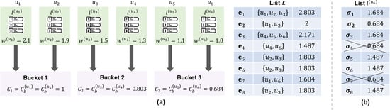
Figure 2.
Indicative examples of the execution of WIRE. The left part demonstrates how the rankers are grouped into buckets and the computation of the confidence and preservation scores (a). The right part illustrates the removal of the weakest elements from an input preference list (b).
The preservation score is a measure of the importance of an element and determines whether it will be included in the aggregate list or whether it will be discarded. Formally, the higher the preservation score of , the higher the probability that will be preserved in . For this reason, the protection score is introduced to determine the number of elements that will be taken into account during the aggregation. Similarly to the confidence score, the protection score is defined for each ranker u according to the following equation:
Equation (8) defines the protection score as an integer threshold that denotes the number of elements of that will contribute during the aggregation process. In other words, it tells us that the weakest elements must be removed from . The item removal process is shown in steps 20–28 of Algorithm 1. For each input list, we build a min-heap structure H to efficiently identify the items to be removed without having to sort . H is built by inserting all elements of and keeps on its head the element with the minimum preservation score. Then, the items with the lowest preservation scores are indicated by performing an equal number of pop operations on H (steps 24–28). The diagram on the right in Figure 2 shows the removal of the two weakest elements from an exemplary input list based on the preservation scores of its elements.
After the removal of the weakest elements from each input list, the aggregator is executed once more on the new lists to obtain the enhanced aggregate list (step 29).
Illustrative Examples. Figure 2 illustrates two examples of how the stages of Algorithm 1 operate in practice. The left part (a) shows the distribution of rankers in equally sized buckets. Initially, each ranker u submits a preference list and a weighted aggregator constructs a consensus ranking by simultaneously assigning weights to all rankers. Setting , the confidence scores for each bucket are computed using Equation (6). Subsequently, the preservation scores of the elements of the aggregate list are computed with Equation (7). For example, the element appeared in the input lists of , , and , which have been previously grouped into buckets 1, 1, and 2, respectively. Therefore, its preservation score will be computed by summing the confidence scores of the following corresponding buckets: .
Having the preservation scores computed, we can now go back to the input lists and remove the weakest elements. First, we need to compute the protection scores for each ranker. The right part of Figure 2 displays an exemplary preference list . Since has been grouped in the bucket , it can be derived that . Therefore, Equation (8) indicates that elements of should be preserved, and 2 elements should be removed. According to the figure, the three elements with the lowest preservation scores are , , and . From these elements, is preserved because it was ranked higher than the other two; and are eventually removed from the list.
Complexity Analysis. In the sequel, we will prove the following lemma:
Lemma 1.
The time complexity of WIRE is upper-bounded by , given that , while it needs space.
Proof.
The cost of sorting the ranker weights (step 1) is . The confidence score calculation (steps 3, 5) takes time. The cost of grouping n rankers (steps 6–11) into buckets is . Calculating the preservation scores of all elements of has worst-case complexity , since each element may appear in all lists.
The last block of Algorithm 1 between steps 20 and 28 includes the construction of n min-heaps H ( worst-case cost), and element removals with a worst-case cost of . Hence, the total worst-case cost of the entire block is .
Consequently, the overall cost of WIRE is expressed as follows:
that can be upper-bounded by , since , , and . Please note that this a quite pessimistic upper bound, since it assumes that every will be excluded from in its entirety.
The space complexity is linear to the number of rankers and the size of the initial aggregate list , since we need to keep all values, all scores, while the maximum size of the auxiliary heap is linear to the length of the longest , which is . □
5. Experiments
This section presents the experimental evaluation of the proposed method. Initially, we describe the datasets, the comparison framework, and the measures that were used during this evaluation. In the sequel, we present and discuss the performance of WIRE against a variety of well-established rank aggregation methods in terms of both effectiveness and running times. We also present a study of how the two hyper-parameters of WIRE, B and , affect its performance. Finally, the statistical significance of the presented measurements is verified in the last part of the section.
The implementation code of the proposed method has been embodied in the FLAGR 1.0.20 and PyFLAGR 1.0.20 (https://flagr.site (accessed on 10 June 2025) libraries [28]. Both libraries are available for download from Github (https://github.com/lakritidis/FLAGR), whereas PyFLAGR can be installed from the Python Package Index (https://pypi.org/project/pyflagr/).
5.1. Datasets
The list pruning strategy of [13] was shown to be effective in scenarios that included long preference lists. However, the experiments have shown that these benefits were diminished, and in some cases, reversed in applications where the preference lists were short. For this reason, in this study, we aimed to examine the performance of WIRE by using not only multiple datasets but also, with diverse characteristics.
In this context, we synthesized six case studies with different numbers of rankers and variable list lengths. We used RASDaGen, an open source dataset generation tool (https://github.com/lakritidis/RASDaGen), to create 6 synthetic datasets that would simulate multiple real-word applications. In particular, we created datasets with long lists to simulate applications related to Bioinformatics (e.g., gene rankings) or Information Retrieval (e.g., metasearch engines). In contrast, the datasets with shorter lists can be considered as representatives of collaborative filtering systems.
In general, finding high-quality datasets with objective relevance judgments is a challenging task. Text Retrieval Conference (TREC) (https://trec.nist.gov/) satisfies these quality requirements, since it annually organizes multiple diverse tracks, accepts ranked lists from the participating groups, and employs specialists to judge the relevance of the submitted items. We used the following two real-world datasets originating from TREC: the Clinical Trials Track of 2022 (CTT22) and the NeuCLIR Technical Docs Track of 2023 (NTDT23). The first one includes 50 topics and 41 rankers, whereas the second one includes 41 topics and 51 rankers. In both datasets, the maximum length of a preference list is limited to 1000 elements.
Table 1 illustrates the attributes of our benchmark datasets. The third column denotes the number of topics for which the rankers submitted their preference lists. The fourth and fifth columns indicate the number of rankers and the length of their submitted lists, respectively. All synthetic datasets have been made publicly available on Kaggle (https://www.kaggle.com/datasets/lakritidis/rankaggregation).

Table 1.
Attributes of the benchmark datasets.
5.2. Comparison Framework and Evaluation Measures
The effectiveness of WIRE was compared against a wide variety of non-weighted and weighted rank aggregation methods. The first set included Borda Count and CombMNZ as they were formalized in [29], the first and the fourth Markov chain-based methods (MC1, MC4) of [19], the Markov chain framework (MCT) of [20], the Robust Rank Aggregation (RRA) method of [21], the Outranking Approach (OA) of [24], the traditional Condorcet [15], and Copeland Winners [30].
The second set included the following four state-of-the-art weighted methods: DIBRA with and without list pruning (termed DIBRA-P and DIBRA, respectively) [13], the weighted approach of [26] based on Preference Relation Graphs (PRGs), and the Agglomerative Aggregation Method (AAM) of [27]. In all methods, we used the same hyper-parameter values as those suggested in the respective studies. Our item removal method was tested in combination with DIBRA, and we refer to it as DIBRA-WIRE in the discussion that follows. In all experiments, we kept the values of the two hyper-parameters of WIRE constant. Therefore, the number of buckets was fixed to , and we set .
The quality of the output lists was measured by employing the following three widespread IR measures: Precision, Normalized Discounted Cumulative Gain (nDCG), and Mean Average Precision (MAP). The first two are computed at specific cut-off points of the aggregate list , and we refer to them as and , respectively. Precision@k is defined as follows:
where is a binary indicator of the relevance of the i-th element of (1/0 for relevant/non-relevant).
On the other hand, nDCG is defined as the Discounted Cumulative Gain (DCG) of divided by the Discounted Cumulative Gain of an imaginary ideal list that has all relevant elements ranked at its highest positions as follows:
Finally, Mean Average Precision (MAP) is defined as the mean of the average precision scores among a set of T topics as follows:
where is the i-th element of the aggregate list , denotes the Precision measured at , and is the total number of relevant entries for the topic .
5.3. Results and Discussion
In this subsection, we present the results of the experimental evaluation of WIRE. In Table 2, Table 3 and Table 4, we report the values of the aforementioned evaluation measures for the 8 datasets of Table 1. More specifically, the second column illustrates the MAP values achieved by the examined methods, the next 5 columns hold the Precision values for the top-5 elements of the produced aggregate list , whereas the last 5 columns denote the nDCG values also for the top-5 elements of .
Table 2.
Performance evaluation of various rank aggregation methods in the MOLO, MASO, and FESO datasets.
Table 3.
Performance evaluation of various rank aggregation methods in the MOSO, MAVSO, and FEVLO datasets.
Table 4.
Performance evaluation of various rank aggregation methods in the CTT22 and NTDT23 datasets.
Now, let us discuss these numbers. At first, the results indicate that DIBRA was the most effective weighted rank aggregation method, achieving the highest MAP scores among the other two methods, PRG and AAM. Interestingly, in all eight cases, our proposed WIRE method managed to further improve the performance of DIBRA by a margin between 1% and 20% (in the FESO dataset). In fact, in most of the examined benchmark datasets, the combination of DIBRA and WIRE outperformed all the competitive aggregation methods, weighted or not.
In the MOLO dataset with the long lists of 100 items, the MAP gain of DIBRA-WIRE compared to DIBRA was roughly 2% ( vs. ). In contrast, the simple list pruning method of [13] offered only infinitesimal improvements in terms of MAP scores. In addition, its effect on the quality of the top-5 elements of the aggregate list was negative in terms of both Precision and nDCG. MC1 and MC4 were also quite effective in this dataset.
The next three datasets, MASO, FESO, and MOSO, were of particular interest, because they involved short lists, and the simple pruning method of [13] is known to perform poorly in such cases. In this experiment, we examined three different scenarios, where variable populations of rankers (i.e., 100, 10, and 50, respectively) submitted short preference lists comprising 30, 10, and 30 items, respectively.
The results were particularly satisfactory in all these scenarios. Compared to DIBRA, our proposed item selection method achieved superior performance in terms of MAP, Precision, and nDCG. For example, the MAP improvements over DIBRA were roughly 1% for MASO and MOSO, and 20% for FESO. Improvements of similar magnitudes were also observed for Precision and nDCG, especially for and . As it was expected, the Mean Average Precision of DIBRA-P was slightly worse compared to that of DIBRA for MASO ( vs. ) and significantly worse in FESO ( vs. ). DIBRA and DIBRA-WIRE were also superior to all the other aggregation methods in all three datasets. The only exception to this observation was MC1 in the FESO dataset, which was superior to DIBRA but inferior to the combination of DIBRA-WIRE.
The fifth case study, abbreviated MAVSO, introduced a scenario that resembles that of a recommender system, namely, numerous rankers submitting very short preference lists of 5 elements. The Outranking Approach of [24] exhibited the best performance in this test, achieving the highest MAP (), , and . Our proposed DIBRA-WIRE method was the second best method, achieving a slightly worse MAP (), , and . The original DIBRA without list pruning outperformed the other two weighted methods, PRG and AAM, but the application of the simple list pruning method of [13] had a strong negative impact on its performance.
The sixth test resembled that of a metasearch engine, with few rankers submitting very long ranked lists of 200 items. Once again, DIBRA-WIRE achieved top performance in terms of MAP (), , and . The method of Copeland Winners and MC4 scored the second highest MAP (i.e., ), but in terms of Precision and nDCG, the aggregate lists created by MCT, RRA, and DIBRA-P were of higher quality. Regarding the weighted methods, DIBRA was more effective than PRG and AAM in terms of Precision and nDCG.
In general, in the six synthetic datasets, the Agglomerative AAM method achieved very low MAP values, but it managed to output decent top-5 rankings. This behavior indicates its weakness in generating high-quality rankings in their entirety. The Preference Relations Graph method was superior to AAM but inferior to DIBRA. On the other hand, the quite old Markov chain-based algorithms were quite strong opponents on datasets with long preference lists (namely, MOLO and FEVLO), but their performance degraded when they were applied to short lists. On average, the Outranking Approach achieved higher MAP values than the Markov Chain methods, but their top-5 rankings were of inferior quality. As mentioned earlier, DIBRA was the most effective rank aggregation method, and our WIRE post-processing step further improved its performance.
Regarding the two real-world datasets, namely, CTT22 and NTDT23, the proposed method was again proved to be beneficial, since it managed to improve the retrieval effectiveness of the baseline DIBRA, even by small margins. On the other hand, the list pruning algorithm of [13] had almost no visible impact in both cases. The order-based methods (i.e., Condorcet, Copeland, and the Outranking Approach) were quite strong opponents to DIBRA and DIBRA-WIRE, producing very qualitative top-5 aggregate lists. In contrast, the three Markov chain-based methods (that performed quite well in the six synthetic datasets) were both ineffective and slow in these two experiments.
The other two weighted aggregation methods had significant difficulties in completing these tests. More specifically, AAM failed to generate consensus rankings in reasonable time, since it required more than 1 h to process one topic from each dataset. In general, AAM was by far the slowest method among all, due to its computationally expensive hierarchical nature. For this reason, and since the TREC datasets were significantly larger than the synthetic ones, Table 4 does not contain results from AAM. On the other hand, PRG is a graph-based memory-intensive algorithm and that became a major bottleneck in the two large TREC datasets. Therefore, a memory starvation error prevented its execution in CTT22. Nevertheless, it managed to complete the aggregation task in all 41 topics of NTDT23, achieving a MAP value of , 17% lower than that of DIBRA.
5.4. Execution Times
In this subsection we examine how WIRE affects the execution time of a weighted rank aggregation method and particularly, DIBRA. Table 5 displays the running times of the involved rank aggregation methods in the benchmark datasets of Table 1. The presented values reveal the running times of each method per topic in milliseconds (recall that each dataset comprises multiple topics).
Table 5.
Execution times (in milliseconds per query) of various rank aggregation methods on the benchmark datasets of Table 1.
These measurements indicate that WIRE imposes only small (and in some cases, infinitesimal) delays in the aggregation process. More specifically, in the six synthetic datasets, Algorithm 1 appended on average only 0.5–2.2 milliseconds to the processing of each query, demonstrating its high efficiency. In fact, DIBRA-WIRE was much faster than (i) the other weighted algorithms, PRG and AAM; (ii) all the order-based techniques (Condorcet and Copeland methods, Outranking approach); and (iii) all the Markov chain-based methods (MC1, MC4, MCT). In contrast, it was slightly slower only than simple linear combination methods like Borda Count and CombMNZ.
As mentioned earlier, in the large TREC datasets, AAM failed to construct aggregate lists in reasonable time (more than one hour per topic). Moreover, PRG consumed all the available memory of our 32 GB workstation in CTT22, also failing to complete the aggregation task. In NTDT23, it was much slower than DIBRA, putting its usefulness into question. This conclusion applies to all the order-based and Markov chain-based methods. Despite their effectiveness in some experiments, the average topic processing times can be 3–5 orders of magnitude larger than those of Borda Count, DIBRA, DIBRA-WIRE, etc.
5.5. Statistical Significance Tests
The reliability of the aforementioned measurements was checked by applying two statistical significance tests. In particular, we executed the Friedman non-parametric statistical test in the measurements of MAP and of all methods. The results of the tests were equal to and , respectively, indicating that the measurements’ distributions exhibit statistically significant discrepancies and that we can reject the null hypothesis.
We also applied the Wilcoxon signed-rank test to examine the pairwise statistical significance of the performances of DIBRA, DIBRA-P, and DIBRA-WISE in terms of Mean Average Precision. The results are presented in Table 6 and indicate that the MAP differences between DIBRA-WIRE and DIBRA are more significant than between DIBRA-P and DIBRA.
Table 6.
Statistical significance of the MAP measurements of DIBRA-WIRE against DIBRA and DIBRA-P. The presented p-values have been obtained by executing the Wilcoxon post hoc signed-rank test.
5.6. Hyper-Parameter Study
The proposed item removal method introduces the following two hyper-parameters: the number of buckets B in which the rankers are grouped, and the parameter of Equation (6). In this subsection, we study how these parameters affect the performance of DIBRA-WIRE, and why the setting of and that was applied in the previous experiment is a choice that, in general, leads to good results.
Our methodology for this study dictated the parallel variation of the values of B and and the independent measurement of MAP in each case. More specifically, for each one of the eight benchmark datasets, we modified B in the range by taking integer steps of 1 at each time (namely, we tested 11 values). Simultaneously we modified in the range by taking steps of at each iteration, also considering 11 values. In other words, we conducted 121 measurements of MAP for each dataset.
The results are illustrated in the heatmaps of Figure 3 and Figure 4. Each heatmap represents the MAP measurements for a different benchmark dataset. The horizontal and vertical axes depict the values of and , respectively. The darker background colors denote higher MAP values, with the black rectangles revealing top performance.
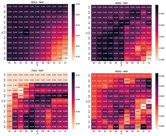
Figure 3.
Hyper-parameter study of DIBRA-WIRE for the MOLO, MASO, FESO, and MOSO datasets. The heatmaps illustrate the fluctuation of Mean Average Precision for variable number of buckets B (horizontal axis) and variable values (in the range ).
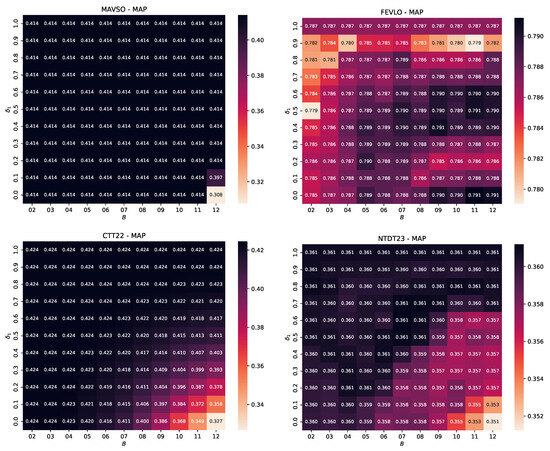
Figure 4.
Hyper-parameter study of DIBRA-WIRE for the MAVSO, FEVLO, CTT22, and NTDT23 datasets. The heatmaps illustrate the fluctuation of Mean Average Precision for a variable number of buckets B (horizontal axis) and variable values (in the range ).
A careful observation of these heatmaps reveals that our choice of and yields satisfactory results in all cases. Of course, there are combinations that “optimize” the performance, but this is not consistent. For example, setting and yielded the best performance in terms of MAP in the MASO dataset. However, this setting does not work well in the FESO dataset. Similarly, and was the best combination for MOSO, but it was also among the worst in the MOLO, MASO, and FESO datasets. For FESO, the best setting was and ; a rather disappointing choice for MOLO and MASO.
We also constructed similar heatmaps for all Precision and nDCG values at the top-5 elements of each aggregate list . Due to space restrictions, we cannot illustrate 80 such diagrams here. Instead, we indicatively choose to depict the fluctuation of against B and in Figure 5 and Figure 6. The results of this exhaustive study verify the conclusions of our previous experiment. Namely, there are multiple combinations of B and that yield decent results, but similarly to the MAP case, there is no “golden rule” achieving top performance in all scenarios. In contrast, one that consistently performs well is and .
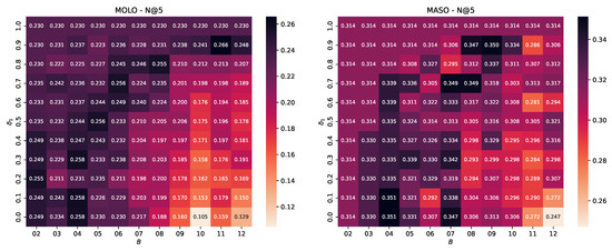
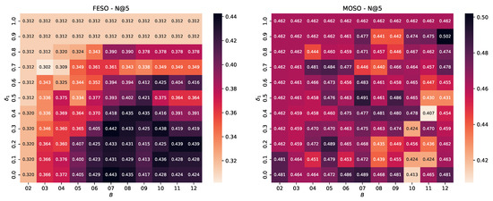
Figure 5.
Hyper-parameter study of DIBRA-WIRE for the MOLO, MASO, FESO, and MOSO datasets. The heatmaps illustrate the fluctuation of for a variable number of buckets B (horizontal axis) and variable values (in the range ).
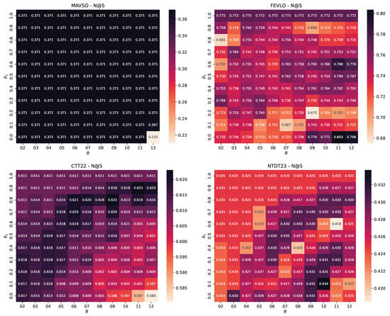
Figure 6.
Hyper-parameter study of DIBRA-WIRE for the MAVSO, FEVLO, CTT22, and NTDT23 datasets. The heatmaps illustrate the fluctuation of for a variable number of buckets B (horizontal axis) and variable values (in the range ).
6. Conclusions and Future Work
In this paper, we introduced WIRE, a novel item selection approach for weighted rank aggregation applications. WIRE functions as a post-processing step to any weighted rank aggregation method and aims to further improve the quality of the output aggregate list. More specifically, our approach initially groups the input preference lists into a pre-defined number of buckets, according to the weights that have been assigned to their respective rankers by the original weighted aggregator. Based on that bucket, each preference list (that is, its respective ranker) is assigned a confidence score that quantifies its importance in a discretized manner.
Then, for each element of the aggregate list, WIRE computes a preservation score that derives from the sum of the confidence scores of the rankers who included it in their preference lists. In the sequel, the aggregate list is sorted in decreasing preservation score order. Consequently, WIRE favors the elements that have been selected by multiple expert rankers. The preservation score is designed to be free of manipulation; therefore, it does not depend on external factors like the individual rankings, pairwise wins and losses, or other score values that may have been assigned by the original aggregator. WIRE also employs the aforementioned confidence scores to compute a threshold value that determines the number of elements to be removed from the (sorted) aggregate list.
Our proposed method was theoretically analyzed and experimentally tested against a collection of 13 state-of-the-art rank aggregation methods in 8 benchmark datasets. The collection included both weighted and non-weighted aggregators, whereas the datasets were carefully selected in order to cover multiple diverse scenarios. The experiments highlighted the high retrieval effectiveness of WIRE in terms of Precision, normalized Discounted Cumulative Gain, and Mean Average Precision. Regarding future work, we intend to enhance WIRE by introducing more sophisticated discretization methods to determine the intervals (and ideally the number) of buckets where the rankers will be grouped. Examples of unsupervised binning methods include buckets of equal widths instead of equally sized buckets, or buckets that derive from the application of a clustering algorithm. We also plan to study alternative mathematical definitions for the confidence, preservation, and protection scores with the aim of improving the effectiveness of WIRE.
Author Contributions
Conceptualization, methodology, software, validation, formal analysis, resources, data curation, writing—original draft preparation, writing—review and editing: L.A. and P.B. All authors have read and agreed to the published version of the manuscript.
Funding
This research received no external funding.
Data Availability Statement
The datasets used in this study are publicly available on Kaggle: https://www.kaggle.com/datasets/lakritidis/rankaggregation. The implementation code of WIRE can be found in the open-source libraries FLAGR 1.0.20 & PyFLAGR 1.0.20: https://flagr.site, https://github.com/lakritidis/FLAGR, https://pypi.org/project/pyflagr/.
Conflicts of Interest
The authors declare no conflicts of interest.
Abbreviations
The following abbreviations are used in this manuscript:
| WIRE | Weighted Item Removal |
| MAP | Mean Average Precision |
| nDCG | normalized Discounted Cumulative Gain |
References
- Chen, J.; Long, R.; Wang, X.l.; Liu, B.; Chou, K.C. PdRHP-PseRA: Detecting remote homology proteins using profile-based pseudo protein sequence and rank aggregation. Sci. Rep. 2016, 6, 32333. [Google Scholar]
- Li, X.; Wang, X.; Xiao, G. A comparative study of rank aggregation methods for partial and top ranked lists in genomic applications. Briefings Bioinform. 2019, 20, 178–189. [Google Scholar] [CrossRef] [PubMed]
- Gyarmati, L.; Orbán-Mihálykó, É.; Mihálykó, C.; Vathy-Fogarassy, Á. Aggregated Rankings of Top Leagues’ Football Teams: Application and Comparison of Different Ranking Methods. Appl. Sci. 2023, 13, 4556. [Google Scholar] [CrossRef]
- Oliveira, S.E.; Diniz, V.; Lacerda, A.; Merschmanm, L.; Pappa, G.L. Is rank aggregation effective in recommender systems? An experimental analysis. ACM Trans. Intell. Syst. Technol. (TIST) 2020, 11, 1–26. [Google Scholar] [CrossRef]
- Bałchanowski, M.; Boryczka, U. A comparative study of rank aggregation methods in recommendation systems. Entropy 2023, 25, 132. [Google Scholar] [CrossRef] [PubMed]
- Akritidis, L.; Katsaros, D.; Bozanis, P. Effective ranking fusion methods for personalized metasearch engines. In Proceedings of the 12th Panhellenic Conference on Informatics, Samos Island, Greece, 28–30 August 2008; pp. 39–43. [Google Scholar]
- Wang, M.; Li, Q.; Lin, Y.; Zhou, B. A personalized result merging method for metasearch engine. In Proceedings of the 6th International Conference on Software and Computer Applications, Bangkok, Thailand, 26–28 February 2017; pp. 203–207. [Google Scholar]
- Akritidis, L.; Katsaros, D.; Bozanis, P. Effective rank aggregation for metasearching. J. Syst. Softw. 2011, 84, 130–143. [Google Scholar] [CrossRef]
- Bartholdi, J.; Tovey, C.A.; Trick, M.A. Voting schemes for which it can be difficult to tell who won the election. Soc. Choice Welf. 1989, 6, 157–165. [Google Scholar] [CrossRef]
- Kilgour, D.M. Approval balloting for multi-winner elections. In Handbook on Approval Voting; Springer: Berlin/Heidelberg, Germany, 2010; pp. 105–124. [Google Scholar]
- Chen, D.; Xiao, Y.; Wu, J.; Pérez, I.J.; Herrera-Viedma, E. A Robust Rank Aggregation Framework for Collusive Disturbance Based on Community Detection. Inf. Process. Manag. 2025, 62, 104096. [Google Scholar] [CrossRef]
- Ma, K.; Xu, Q.; Zeng, J.; Liu, W.; Cao, X.; Sun, Y.; Huang, Q. Sequential Manipulation Against Rank Aggregation: Theory and Algorithm. IEEE Trans. Pattern Anal. Mach. Intell. 2024, 46, 9353–9370. [Google Scholar] [CrossRef] [PubMed]
- Akritidis, L.; Fevgas, A.; Bozanis, P.; Manolopoulos, Y. An unsupervised distance-based model for weighted rank aggregation with list pruning. Expert Syst. Appl. 2022, 202, 117435. [Google Scholar] [CrossRef]
- de Borda, J.C. Mémoire sur les élections au scrutin. In Histoire de l’Academie Royale des Sciences; Imprimerie Royale: Paris, France, 1781; pp. 657–665. [Google Scholar]
- De Condorcet, N. Essai sur l’Application de l’Analyse à la Probabilité des Décisions Rendues à la Pluralité des Voix; Imprimerie Royale: Paris, France, 1785. [Google Scholar]
- Emerson, P. The original Borda Count and partial voting. Soc. Choice Welf. 2013, 40, 353–358. [Google Scholar] [CrossRef]
- Montague, M.; Aslam, J.A. Condorcet fusion for improved retrieval. In Proceedings of the 11th ACM International Conference on Information and Knowledge Management, McLean, VA, USA, 4–9 November 2002; pp. 538–548. [Google Scholar]
- Li, G.; Xiao, Y.; Wu, J. Rank Aggregation with Limited Information Based on Link Prediction. Inf. Process. Manag. 2024, 61, 103860. [Google Scholar] [CrossRef]
- Dwork, C.; Kumar, R.; Naor, M.; Sivakumar, D. Rank aggregation methods for the Web. In Proceedings of the 10th International Conference on World Wide Web, Hong Kong, China, 1–5 May 2001; pp. 613–622. [Google Scholar]
- DeConde, R.P.; Hawley, S.; Falcon, S.; Clegg, N.; Knudsen, B.; Etzioni, R. Combining results of microarray experiments: A rank aggregation approach. Stat. Appl. Genet. Mol. Biol. 2006, 5, 15. [Google Scholar] [CrossRef] [PubMed]
- Kolde, R.; Laur, S.; Adler, P.; Vilo, J. Robust rank aggregation for gene list integration and meta-analysis. Bioinformatics 2012, 28, 573–580. [Google Scholar] [CrossRef] [PubMed]
- Kemeny, J.G. Mathematics without numbers. Daedalus 1959, 88, 577–591. [Google Scholar]
- Young, H.P.; Levenglick, A. A consistent extension of Condorcet’s election principle. SIAM J. Appl. Math. 1978, 35, 285–300. [Google Scholar] [CrossRef]
- Farah, M.; Vanderpooten, D. An outranking approach for rank aggregation in information retrieval. In Proceedings of the 30th ACM Conference on Research and Development in Information Retrieval, Amsterdam, The Netherlands, 23–27 July 2007; pp. 591–598. [Google Scholar]
- Pihur, V.; Datta, S.; Datta, S. Weighted rank aggregation of cluster validation measures: A Monte Carlo cross-entropy approach. Bioinformatics 2007, 23, 1607–1615. [Google Scholar] [CrossRef] [PubMed]
- Desarkar, M.S.; Sarkar, S.; Mitra, P. Preference relations based unsupervised rank aggregation for metasearch. Expert Syst. Appl. 2016, 49, 86–98. [Google Scholar] [CrossRef]
- Chatterjee, S.; Mukhopadhyay, A.; Bhattacharyya, M. A weighted rank aggregation approach towards crowd opinion analysis. Knowl.-Based Syst. 2018, 149, 47–60. [Google Scholar] [CrossRef]
- Akritidis, L.; Alamaniotis, M.; Bozanis, P. FLAGR: A flexible high-performance library for rank aggregation. SoftwareX 2023, 21, 101319. [Google Scholar] [CrossRef]
- Renda, M.E.; Straccia, U. Web metasearch: Rank vs. Score based rank aggregation methods. In Proceedings of the 2003 ACM Symposium on Applied Computing, Melbourne, FL, USA, 9–12 March 2003; pp. 841–846. [Google Scholar]
- Copeland, A.H. A Reasonable Social Welfare Function; Technical Report; University of Michigan: Ann Arbor, MI, USA, 1951. [Google Scholar]
Disclaimer/Publisher’s Note: The statements, opinions and data contained in all publications are solely those of the individual author(s) and contributor(s) and not of MDPI and/or the editor(s). MDPI and/or the editor(s) disclaim responsibility for any injury to people or property resulting from any ideas, methods, instructions or products referred to in the content. |
© 2025 by the authors. Licensee MDPI, Basel, Switzerland. This article is an open access article distributed under the terms and conditions of the Creative Commons Attribution (CC BY) license (https://creativecommons.org/licenses/by/4.0/).