1. Introduction
Soil salinization is one of the key environmental problems directly affecting crops, ecosystem functioning, and regions’ water regimes [
1,
2,
3]. In climate change conditions and agricultural land use intensification, the extent of soil degradation [
4,
5,
6] increases incredibly rapidly. Hence, developing effective monitoring and prediction tools for salinity is imperative. Satellite data, in particular multi-band images from Sentinel-2 platforms [
7], combined with climate models such as ERA5-Land, provide extensive information on the state of the soil cover. Still, their processing requires modern data analysis methods [
8]. Currently, the scientific literature presents various approaches to assessing soil salinity, including spectral indices such as NDVI, NDWI, and NDSI [
9,
10], as well as machine learning using classification [
11] and regression [
12,
13] methods. However, classical supervised learning methods face significant challenges due to the lack of reliable ground-truth labels and the heterogeneity of spectral feature distributions. Additionally, several limitations of the proposed approach must be acknowledged. Due to atmospheric scattering effects, the performance of spectral indices may deteriorate under dense vegetation or in the presence of high aerosol content. Moreover, the spatial resolution of ERA5-Land climate covariates remains coarse for detailed local analysis, and comprehensive in situ soil salinity and conductivity validation is still in progress. These factors may limit the model’s generalizability beyond arid and semi-arid environments.
In this regard, in recent years there has been an increased interest in hybrid methods combining unsupervised algorithms, ensemble techniques, and deep neural networks to improve forecasting accuracy. One of the pressing challenges in this area is the need to consider the spectral features of different soil types, including saline, regular, and sandy soils, since the spectral characteristics of sandy soils can overlap with signals from saline areas. Moreover, an important task is developing algorithms that can adaptively segment data in high spatial and spectral variability conditions. In this paper, we propose a hybrid model combining unsupervised algorithms (K-Means [
14,
15], agglomerative clustering, DBSCAN [
16,
17]) with supervised methods (XGBoost [
18,
19,
20], multi-task neural network). The initial stage involves clustering the data using the K-Means method to form pseudo-labels, which are then used to train an XGBoost model that calculates the probabilities of objects belonging to specific classes. These pseudo-labels represent a coarse three-class partitioning of the input dataset, where each pixel is assigned to one of the clusters based on spectral similarity. Although these clusters do not correspond to expert-annotated labels, they serve as surrogate target variables that guide the learning process of the subsequent supervised model. This semi-supervised strategy allows leveraging large volumes of unlabeled remote sensing data while preserving meaningful structural groupings in the feature space. Next, an ensemble approach is applied with the voting of several clustering algorithms, after which the final labels are used to train a multi-task neural network that simultaneously solves the problems of classification and regression of soil salinity.
The study hypothesizes that the proposed approach will provide more accurate soil segmentation by salinity compared to traditional clustering and classification methods. The experiments will evaluate key metrics of the model quality, including the Silhouette Score, Davies–Bouldin Score, Calinski–Harabasz Score, and the impact of the hybrid ensemble on the quality of the final predictive model. The study’s main findings are that applying the hybrid approach improves the accuracy of salt-affected soil segmentation, minimizes the influence of boundary effects between different soil cover types, and adapts the model to the spatial heterogeneity of the data. This study assists in enhancing soil remote sensing methods and can be utilized to monitor land degradation in the salinized region. Soil salinization is an environmentally significant problem affecting cultivated fields’ productivity, ecosystem functions, and water. The urgency to create soil salinity monitoring and prediction tools is gradually increasing due to climate change and the escalating development of agriculture. Scientists have recently attempted to integrate satellite imaging, machine learning algorithms, and geographic information systems to improve soil salinity prediction and mapping accuracy. One of the new fields of study is using remote sensing and spectral indicators to detect soil salinity. The study [
21] analyzed methods for automatically detecting saline lands using Sentinel-2 data and deep learning algorithms. The results showed that combining spectral indices (NDVI, NDSI, BI) with multilayer neural networks allows for the high classification accuracy of saline soils (up to 91.2%). Another study [
22] proposed an improved methodology for using hyperspectral data to analyze soil conditions. The data were processed using transformer methods, allowing more accurate modeling of spatiotemporal patterns of salinity changes. In addition, various approaches to integrating climate data and satellite images to predict soil salinity dynamics are being studied. For example, the work [
23] proposes a method based on machine learning and ERA5-Land model data that allows predicting changes in soil degradation, taking into account changes in soil temperature and moisture. Ensemble methods, such as gradient boosting and random forest, increased the forecasting accuracy by 15% compared to traditional linear regression models. Another critical area of research is the assessment of agricultural land degradation due to soil salinization. The study [
24] presents an approach based on multispectral sensing and machine learning that allows quantifying the degree of soil salinity in arid regions. The authors emphasize that combining unsupervised methods (K-Means clustering, DBSCAN) with supervised methods (XGBoost, neural networks) allows for minimizing classification errors and considering complex nonlinear dependencies in soil characteristics.
In addition to remote sensing, approaches based on local measurements and modeling of salinization processes are actively being developed. The study [
25] analyzed the possibilities of combining uncrewed aerial vehicle (UAV) data with geostatistical models for mapping soil salinity. The work shows that UAVs, in combination with deep learning methods, can reduce monitoring costs while providing high spatial accuracy. Finally, the study [
26] considers an integrated approach combining satellite monitoring, ground-based measurements, and machine learning to predict soil salinity in different regions. The authors emphasize that using ensemble models increases the reliability of forecasts, especially in conditions of limited availability of field data. Thus, modern research demonstrates significant progress in monitoring and forecasting soil salinity. Integrating remote sensing data, climate models, and machine learning algorithms allows the enhancement of the accuracy of saline land classification and the development of predictive models based on spatiotemporal dynamics of soil properties. These are required for sustainable land management, reducing the impacts of soil degradation, and improving agricultural production efficiency.
2. Materials and Methods
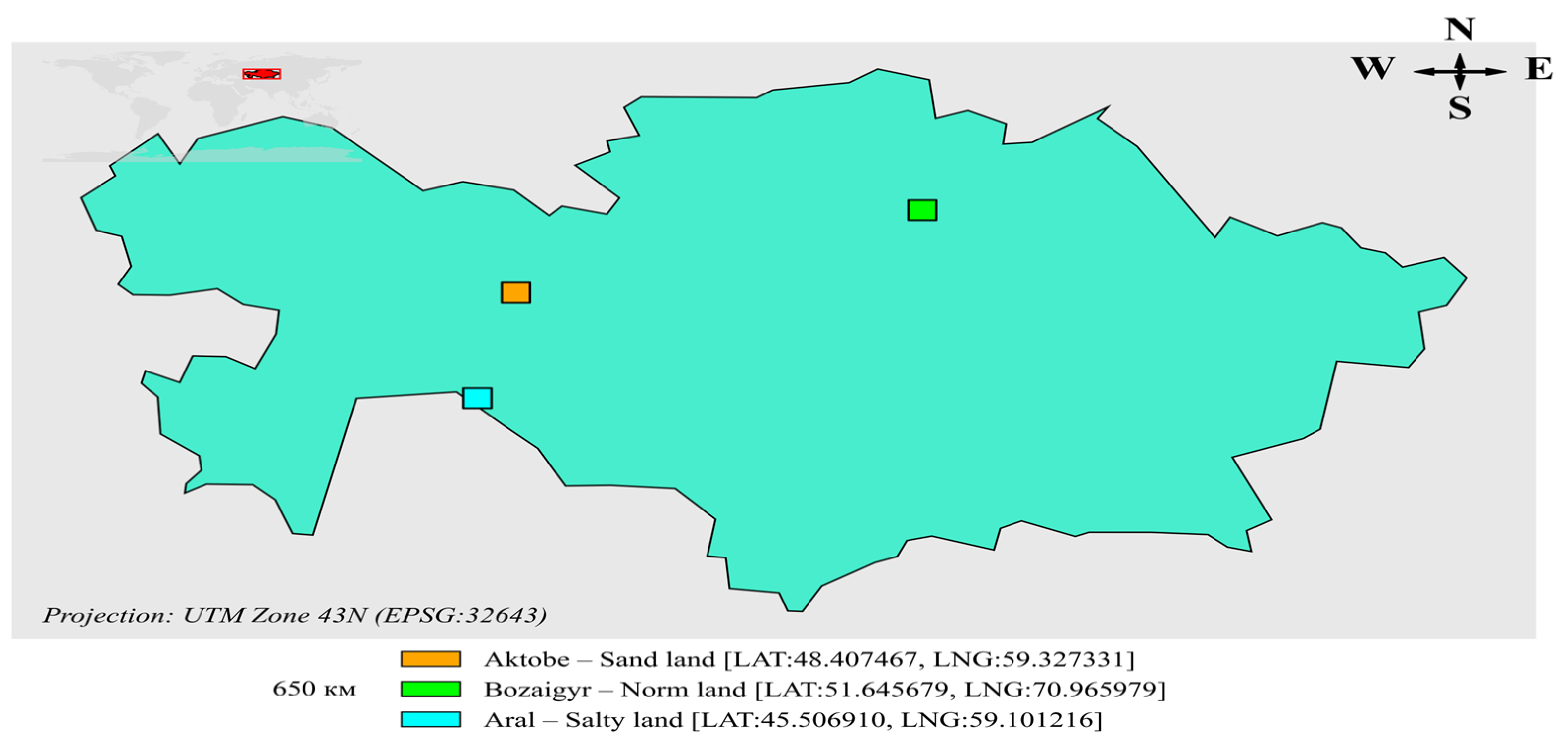
The study applied multi-band Sentinel-2 satellite imagery and ERA5-Land climate model data. The spectral bands of Sentinel-2 used in the research were B2, B3, B4, B8, B8A, B11, and B12, with derived indices like NDVI, NDWI, NDSI, SI1–SI5, and BI for analysis of vegetation cover, soil moisture, and surface mineralization. Soil water volume content (VSWL1–VSWL4) was taken from the ERA5-Land model for four depths (0–7 cm, 7–28 cm, 28–100 cm, and 100–289 cm) to take into account the influence of water on salinity processes. Three geographically diverse regions were selected for investigation: the previous bottom of the Aral Sea (high salinity), Bozaigyr village in the Akmola region (moderate salinity and typical vegetation), and Shol in the Aktobe region (sandy soil with sparse vegetation), which allowed for testing in full on diverse grounds. A map of these sites superimposed on a Sentinel-2 background with EPSG:32643 coordinates is presented in
Figure 1. The dataset covers 2019–2024 and comprises multi-seasonal images from April to October (2019–2021), which capture pre-cultivation, vegetative, and post-harvest growth stages. This setup captures spatial and seasonal variation, thus enhancing the robustness and generalizability of the model.
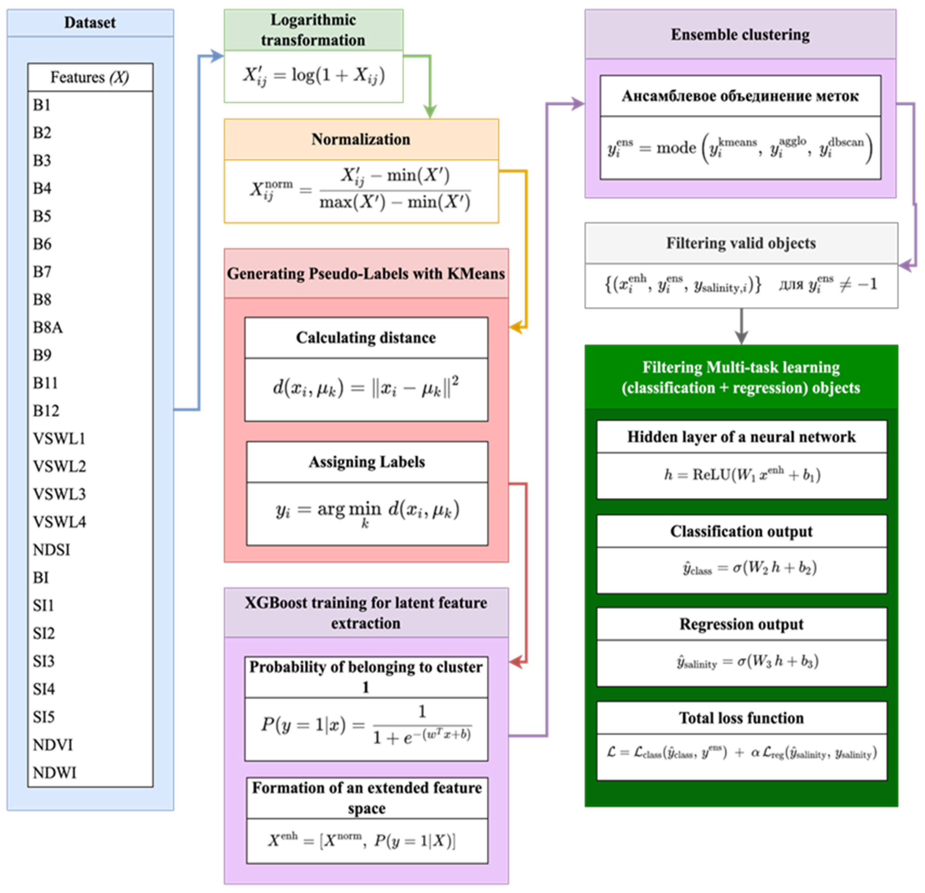
Figure 2 illustrates the methodology of this approach to soil salinity clustering and prediction that combines machine learning methods. The flow chart shows the sequential data processing stages, from preprocessing and pseudo-label creation to ensemble learning and multi-task neural modeling.
1. The first stage of the study involves preprocessing the data. The initial data are prepared for further analysis at this stage, including eliminating the distribution’s asymmetry and bringing the features to a single scale. First, a logarithmic transformation is applied, which reduces the impact of outliers and the skewness of the distribution. Next, the data are normalized so all features have values in the range [0, 1]. This improves subsequent algorithms’ convergence and ensures each feature’s uniform influence on the model.
2. Logarithmic transformation (1):
where
—is the original value of the
-th feature of object
i, where
,
—prime is the transformed value after applying the logarithm,
.
3. Normalization (2):
where
—prime is the feature matrix after logarithmic transformation;
—is the normalized feature matrix, where the values are brought to the range from 0 to 1.
4. After data preprocessing, pseudo-labels are generated using the K-Means algorithm. At this stage, the K-Means algorithm is used to initially split the normalized data
into two clusters. The algorithm calculates the cluster centers and assigns a label to each point based on the minimum distance to the nearest center. The resulting pseudo-labels are used as a guide for further training the XGBoost model, providing the initial data splitting (3) and label assignment (4).
where
—is the feature vector of the i-th object from
;
—is the center of cluster
, where
= 1, 2,
—is the square of the Euclidean distance between
и
.
where
—are the calculated distances for each object
to the cluster centers,
—is the cluster index, and
, y_i—is the pseudo-label assigned to the
-th object,
.
5. In this step, XGBoost is trained on normalized data with pseudo-labels to obtain probabilistic membership estimates in a particular cluster. These probabilities reflect hidden patterns in the data that are not captured by simple clustering methods. Result (probability
(5) is added to the original features, forming an extended feature space
(6).
where
—is a feature vector from
,
—is a vector of model weights,
—is (bias), and
—is the probability of object
belonging to class 1; the value is in the range [0, 1].
where
—is the normalized data,
—is the probability vector for each object obtained by formula (6), and
—is the extended feature matrix containing the original features and an additional probability feature,
.
6. The next step is to apply ensemble clustering. In this step, the extended feature space
is used to apply three clustering methods in parallel: K-Means, agglomerative clustering, and DBSCAN. Each method independently assigns labels to objects, and then the results are combined using a voting procedure, where the final label for an object is determined as the most frequently occurring value. This ensemble approach reduces the impact of the individual errors of each method and provides a more stable and accurate partitioning of the data (7).
where
—label assigned to an object
algorithm K-Means,
—label assigned to an object
agglomerative clustering,
—label assigned to an object
algorithm DBSCAN, and
—final ensemble label for the object
,
.
7. After ensemble clustering, some objects may receive the label “noise” (−1), so only objects with valid labels are selected for further training. The input of the multi-task model will be the extended features
(for the selected objects), as well as two target variables: (1) the class
for classification, and (2) the salinity pseudo-label
(in our case, the probability returned by XGBoost for class 1, or other available salinity estimates) (8).
where
—are extended features,
—are ensemble labels, and
—are pseudo-labels (or accurate labels) of salinity.
The choice of K-Means, Agglomerative Clustering, and DBSCAN, followed by supervised methods (XGBoost and multi-task neural network), is motivated by the need to segment soil types under uncertainty robustly and the absence of ground-truth labels. K-Means provides an initial coarse clustering based on centroid distances, ensuring fast and stable pseudo-labeling. However, its spherical bias limits accuracy in irregular-shaped distributions. Therefore, Agglomerative Clustering is added to refine cluster boundaries in such complex regions. DBSCAN complements the pipeline by detecting and excluding outliers and noise points (e.g., scattered “salt spots”), forming a denser and more reliable cluster core. Ensemble voting across the three clustering methods reduces the influence of each algorithm’s individual bias and stabilizes label assignment. These pseudo-labels are then used to train an XGBoost model, which converts hard labels into probabilistic soft outputs, uncovering nonlinear feature interactions. The extended feature space, enriched with these probabilities, is passed to a multi-task neural network trained to classify soil types and regress salinity levels simultaneously.
The final stage is multi-task learning, combining classification and regression. A neural network is used that simultaneously solves two problems: classification by ensemble labels
regression by the pseudo-label of
. The model contains a standard input layer, several hidden layers (9), and then two “heads”—the output for classification (10) and the output for regression (11). The loss functions (12) for both problems are jointly considered during training.
where
—is the extended feature vector for one object,
—is the weight matrix and bias vector of the first hidden layer, and
—is the activation of the hidden layer (new feature representation).
where
is the hidden layer output,
—are the parameters of the classification layer,
, and
—is the probability of belonging to class 1.
where
—is the output of the hidden layer,
—are the parameters of the regression layer,
—is used here as a limiter that brings the prediction to the range [0, 1], and
—is the predicted salinity value.
where
,
—are the predicted and actual labels for classification,
—are the predicted and actual (or pseudo) salinity labels,
—is a weight constant that determines the contribution of the regression problem to the total error, and
—is the final loss function used in training the neural network.
The following software was used for implementation: Python 3.9.12, TensorFlow 2.12.0 for neural networks, XGBoost 1.6.2 for gradient boosting, Scikit-learn 1.1.3 for clustering and normalization, GDAL 3.4.0 for geodata processing, Matplotlib 3.5.2, and Seaborn 0.11.2 for visualization. Satellite image data were acquired and processed using the Google Earth Engine API. Models were executed on a computation server equipped with an NVIDIA RTX 3090 graphics card (24 GB VRAM) and 128 GB of RAM, sourced from NVIDIA Corporation, Santa Clara, CA, USA, to ensure high computational performance and large data capacity. Satellite data from Sentinel-2 are accessed through the Copernicus Open Access Hub (
https://www.copernicus.eu/en) (accessed on 20 March 2025). ERA5-Land climate data are accessed from the ECMWF Climate Data Store (
https://cds.climate.copernicus.eu) (accessed on 20 March 2025). Thus, the proposed method can be reproduced and adapted for other regions, which makes it a universal tool for soil salinity analysis.
The model is based on two supplementary sources of information: Sentinel-2 multispectral imagery and climate ERA5-Land model data. We utilized both to consider surface reflectance properties and hydrology affecting salinization. The European Space Agency’s Sentinel-2 satellite system of the Copernicus program has a multispectral sensor MSI with high-resolution imaging in the wide part of the spectrum (10–60 m). The analysis used 10 m resolution bands: B2 (blue), B3 (green), B4 (red), B8 and B8A (short-wave infrared), and B11 and B12 (mid infrared). These data are necessary to assess vertical salt transport processes, i.e., leaching or build-up as a function of depth and season. In addition to the fundamental spectral and hydrologic properties, the model included derived spectral indices (SI1–SI5, NDVI, NDWI, NDSI, BI) that increased the model’s sensitivity to vegetation and soil moisture properties. Thus, the set of features covers surface and deep parameters, providing a comprehensive approach to salinity modeling. This expands the analysis capabilities and increases the method’s versatility when applied in various natural and climatic conditions. The data were obtained through Google Earth Engine. The following indices were used in this work:
1. Normalized Differential Salinity Index (NDSI) (13):
where
—is the value of the red channel (B4);
—is the near infrared channel (B8). This index is used to assess the level of soil salinity.
2. Brightness Index (BI) (14):
This index reflects the surface brightness and helps estimate the soil texture.
3. Salinity Index 1 (SI1) (15):
where B is the value of the blue channel (B2).
4. Salinity Index 2 (SI2) (16):
where
G is the value of the green channel (B3).
5. Salinity Index 3 (SI3) (17):
where SWIR1 and SWIR2—are the values of the middle infrared channels (B11 and B12).
6. Salinity Index 4 (SI4) (18):
7. Salinity Index 5 (SI5) (19):
8. Normalized Difference Vegetation Index (NDVI) (20):
9. Normalized Difference Water Index (NDWI) (21):
3. Results and Discussion
The proposed method demonstrated high efficiency in forecasting and spatial segmentation of soil salinity. In contrast to the basic approach based solely on the K-Means algorithm, the developed system, combining ensemble clustering, probabilistic feature enrichment, and multi-task neural network architecture, showed significant improvement in all key metrics. This confirms the feasibility of integrating machine learning methods when processing complex heterogeneous data typical for remote monitoring tasks. The model is based on two complementary data sources: Sentinel-2 multispectral imagery and climate data from the ERA5-Land model. We utilized both to capture surface reflectance properties and hydrology that affect salinization. The European Space Agency’s Sentinel-2 satellite system under the Copernicus initiative carries a multispectral sensor MSI offering imaging with high spatial resolution in a vast portion of the spectrum (10–60 m). The analysis utilized 10 m resolution bands: B2 (blue), B3 (green), B4 (red), B8 and B8A (short-wave infrared), and B11 and B12 (mid infrared). These channels provide information on vegetation cover, humidity, and reflective characteristics of the surface, including hints on mineral composition and potential salinity.
We conducted performance testing in both local and cloud computing environments to evaluate the model’s suitability for real-world deployment. The tests focused on key metrics such as inference time, processing throughput, memory consumption, and scalability.
Table 1 below summarizes the results of two representative platforms: a local Apple M1 Pro system and a cloud-based NVIDIA RTX 3090 server.
The model demonstrates high computational efficiency, with inference times under 1.2 s per tile and throughput exceeding 1 megapixel per second in a parallelized setup. The complete processing of a 100 km2 scene requires less than two minutes in a cloud environment, while the entire Sentinel-2 scene (~120 MPix) can be processed in under 2.5 min using 32-thread queues. The low memory usage (~0.2 GB) and modular structure of the pipeline ensure excellent scalability, making the system well-suited for near real-time applications in large-scale remote sensing and monitoring tasks.
These indices play a key role in assessing the condition of the soil, since they directly reflect such indicators as the salinity level and water balance of the upper horizon. The study processed a total of 33,624 rows of data. Of the total dataset containing 33,624 observations, 23,536 rows were used for model training, while the remaining 10,088 rows were allocated for testing and clustering quality assessment. The 23,536:10,088 split (approximately 70:30) is justified through stratified sampling, which preserves the natural class distribution of 34% saline soils, 46% normal soils, and 20% sandy soils. This approach ensures that each class is sufficiently represented in the test set, with at least 1500 observations per class, thereby supporting a confidence interval of ±1% for accuracy estimates.
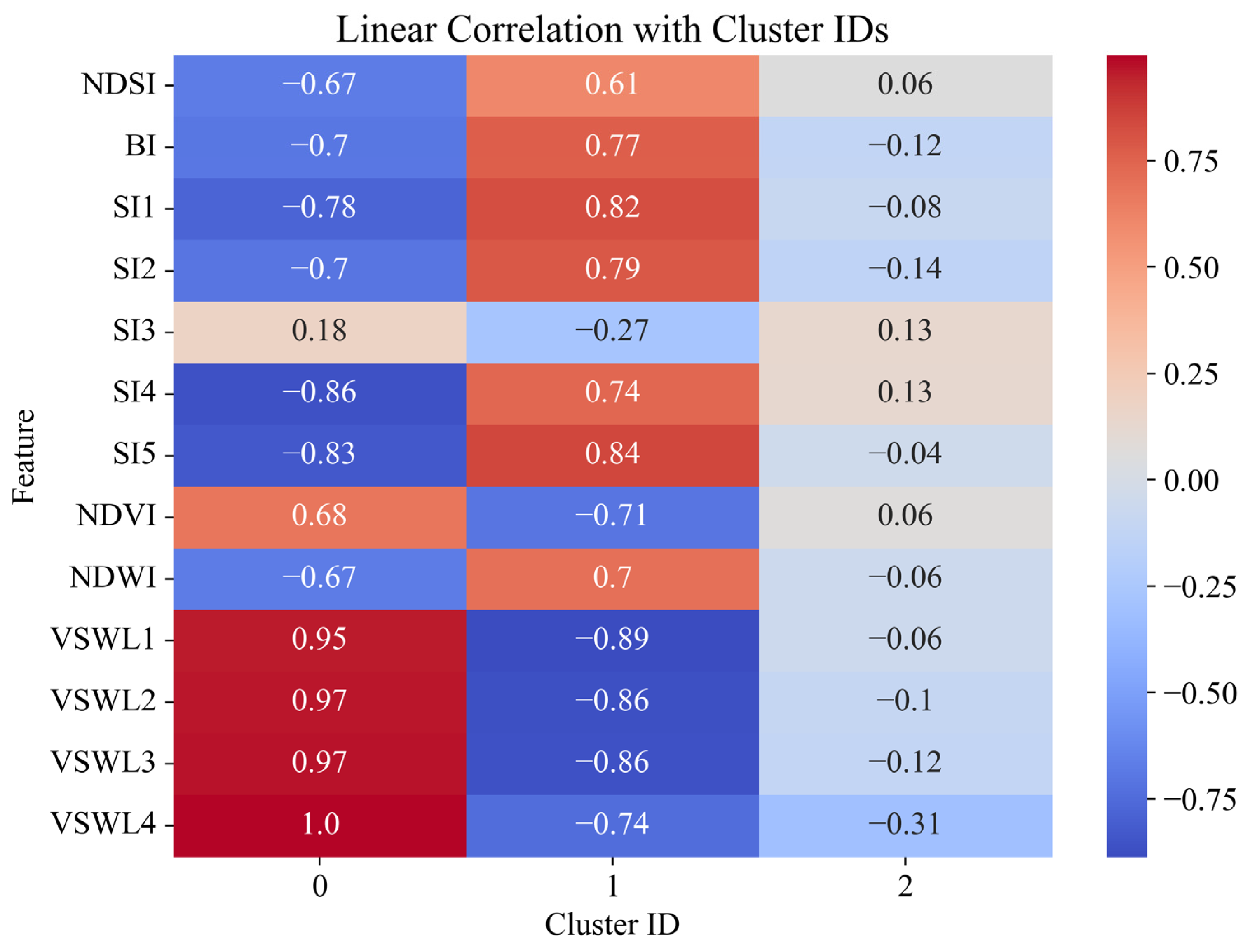
Figure 3 shows a heat map of the linear correlation between the features and pseudo-labels of the clusters (Pseudo-Label Index) obtained from clustering. The
Y-axis shows the used features, including spectral indices (NDSI, NDVI, NDWI, SI1–SI5, BI) and the hydrological ERA5-Land model variables (VSWL1–VSWL4), whereas the
X-axis shows the cluster indices (0, 1, 2). The color scale represents the correlation level: positive values are shown in red hues, indicating a direct relation, and negative ones are shown in blue, suggesting an inverse relationship. The strongest positive correlation with cluster 0 is observed for all hydrological variables (VSWL1–VSWL4), with VSWL4 (1.00) indicating an association of high soil moisture levels with this cluster type. At the same time, for cluster 1, most features (in particular, SI1, SI2, SI5, and NDVI) demonstrate a positive correlation, which may indicate spectral features of salinity. Cluster 2 is characterized by weak or slightly negative correlations, which may indicate its intermediate or mixed nature. Such visualization allows a better understanding of the contribution of individual features to cluster formation and the interpretation of the physical properties of different soil types identified during clustering.
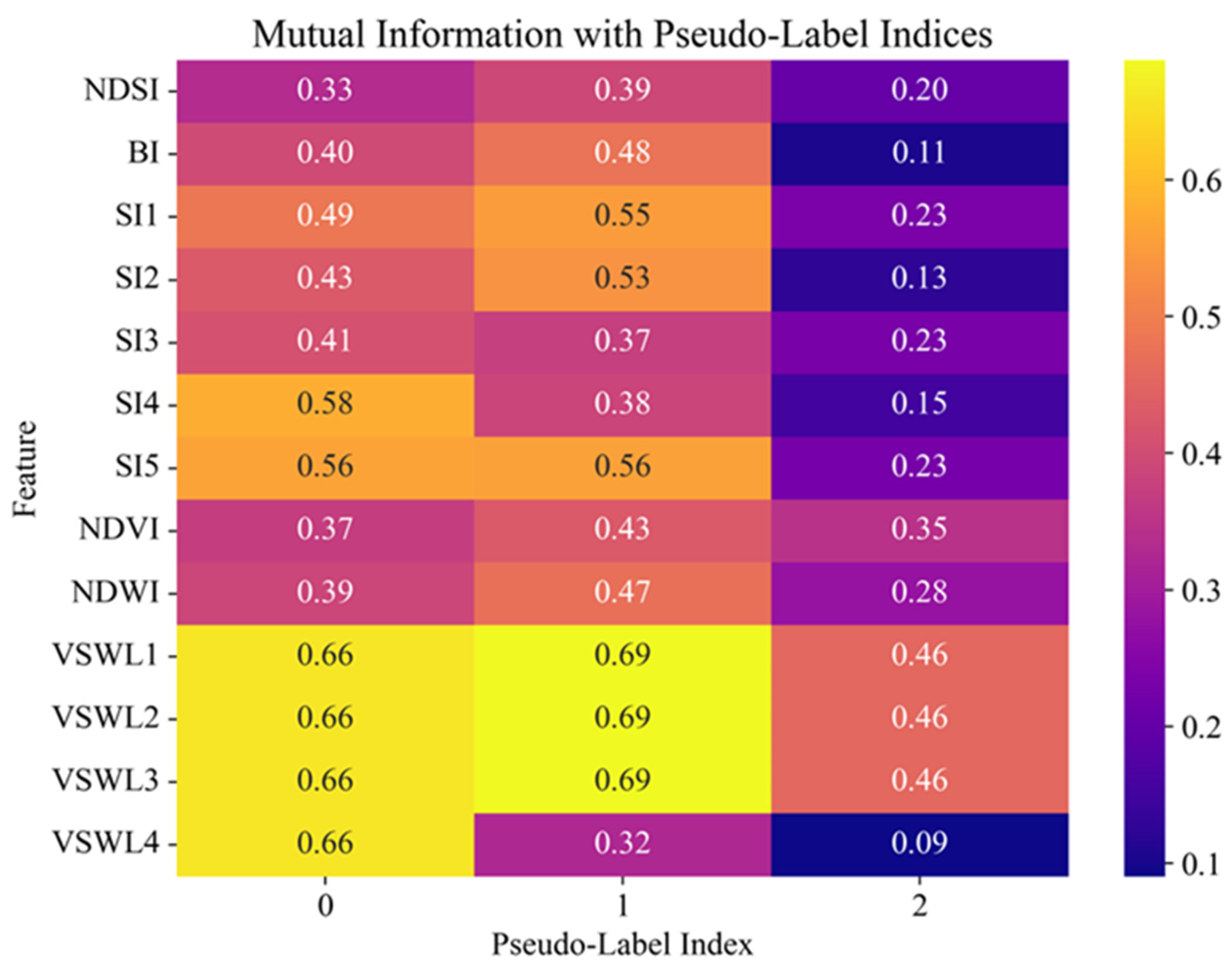
Figure 4 shows the heat map of mutual information between the features and pseudo-label indices of clusters obtained in the clustering process. The vertical axis shows the features, including spectral indices (NDSI, SI1–SI5, NDVI, NDWI, BI) and hydrological parameters (VSWL1–VSWL4), and the horizontal axis shows the cluster indices (0, 1, 2). The color scale displays the value of mutual information, where brighter yellow shades correspond to a high level of informativeness of the feature regarding cluster membership. Hydrological parameters VSWL1, VSWL2, and VSWL3 for clusters 0 and 1 (0.69) attain maximum mutual information values, confirming their substantial value towards separating the data by the soil moisture level. Among the spectral characteristics, SI4, SI5, and SI1 have the highest mutual information with the labels, especially concerning cluster 0 and cluster 1, and thus are most significant in identifying soil salinity and texture. Mutual information for each feature compared with cluster 2 is lower, which might indicate a less structured or mixed nature of cluster 2. Thus, visualization of mutual information allows us to see the most significant features contributing to the generation of the cluster structure and can be used for additional feature selection and model interpretation.
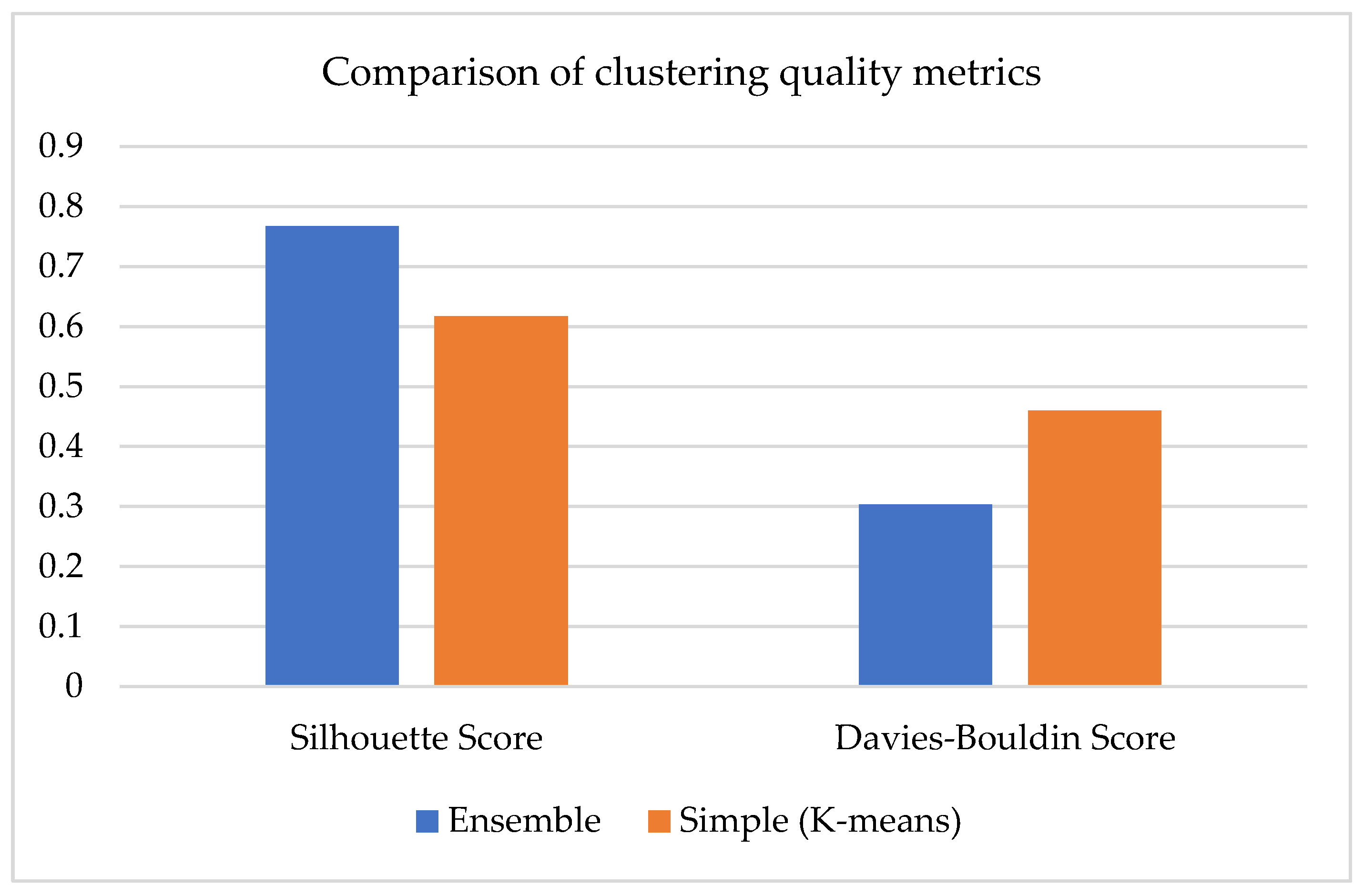
Figure 5 compares the clustering quality of two models: one simpler with the K-Means algorithm (orange bars) and an ensemble model (blue bars) that combines multiple methods. Two internal evaluation metrics were used: Silhouette Score and Davies–Bouldin Score. The Silhouette Score, which describes how isolated the clusters are, was higher in the ensemble model (0.76754) than in the simple model (0.61703), illustrating increased separation between clusters of objects. Meanwhile, a low Davies–Bouldin Score is better. This score was smaller in the ensemble technique (0.30375 versus 0.46008), illustrating more cluster compactness and less overlapping. These measurements confirm that the ensemble model achieves better quality clustering than the baseline K-Means algorithm.
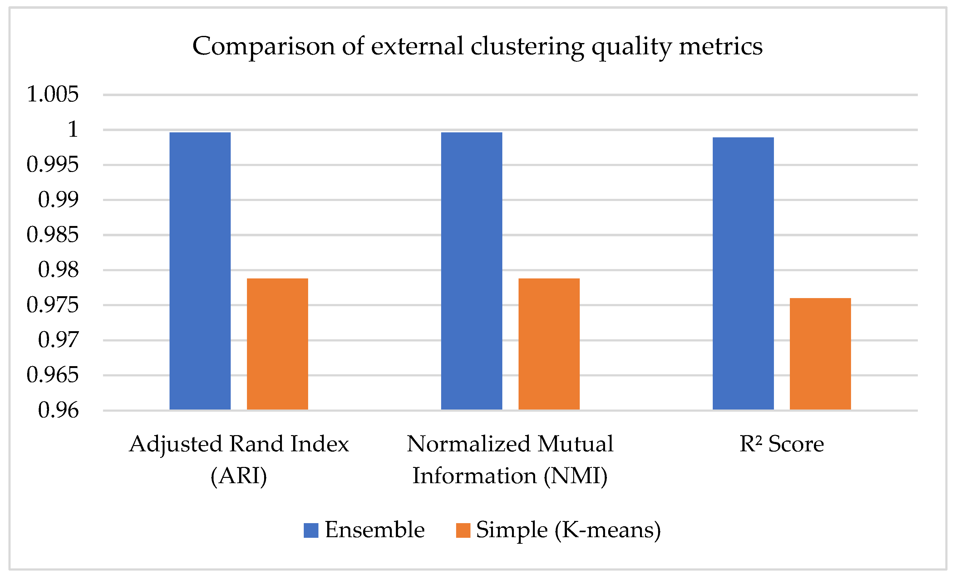
Figure 6 compares external clustering quality metrics for two approaches: a simple model based on the K-Means algorithm (orange bars) and an ensemble model (blue bars) using a combined clustering approach. The Adjusted Rand Index (ARI), Normalized Mutual Information (NMI), and the coefficient of determination (R
2 Score) were used as evaluation metrics. All indicators demonstrate a significant advantage of the ensemble model. Thus, the ARI and NMI values were 0.9996 for the ensemble versus 0.97879 for K-Means, indicating a high match with the proper labels and greater informativeness of clustering. Similarly, the R
2 Score value—0.99889 for the ensemble and 0.976 for K-Means—indicates a better explanatory power of the model. Thus, the ensemble approach provides a more accurate match of the clusters to the real data structure, which all three metrics confirm.
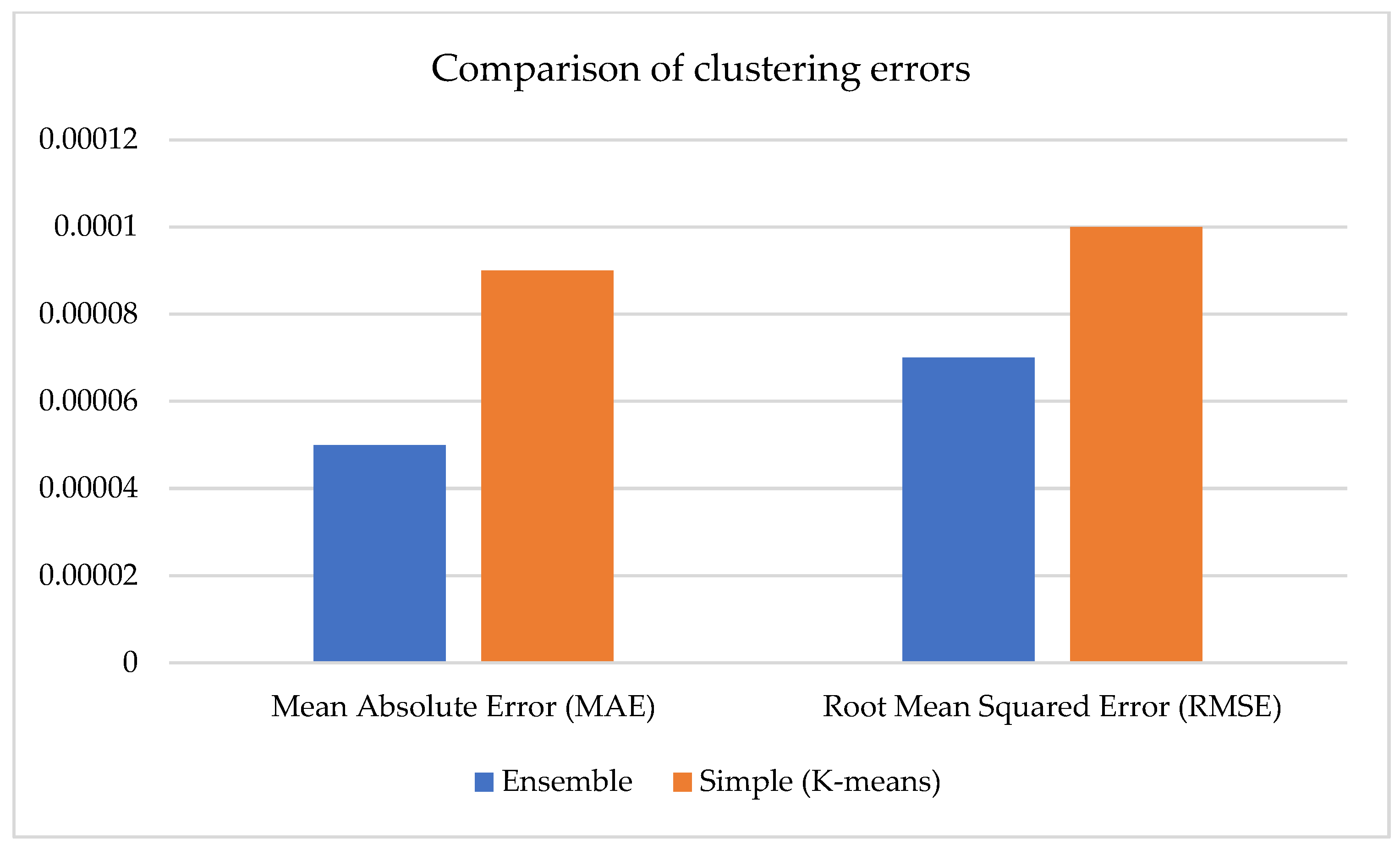
Figure 7 compares clustering errors for two approaches: the basic model using the K-Means algorithm (orange bars) and the ensemble model (blue bars) combining several methods. Root mean square error (RMSE) and mean absolute error (MAE) were employed as measures, which enabled us to compare the difference between predicted and reference values. It can be noticed that the ensemble model possesses considerably smaller error values: MAE approximates 0.00005 vs. 0.00009 for the simple model, and RMSE approximates 0.00007 vs. 0.0001. This indicates more accurate forecasting and a closer approximation of the model to the actual data distribution. Thus, the ensemble approach provides structurally more apparent clustering and reduces numerical errors, which is especially important when applying the model to regression analysis problems or quantitative assessment of features, such as the degree of soil salinity.
The higher Silhouette Score value of the ensemble model (0.76754 versus 0.61703 for the simple K-Means model) indicates better clustering quality—objects within a cluster are located more compactly, and the distances between clusters are increased. This means the proposed algorithm designs better data partitioning: objects with the same cluster are more similar, while differences between clusters are enhanced. Furthermore, the decrease from the Davies–Bouldin Score of 0.46008 by K-Means to 0.30375 of the ensemble solution indicates a tighter overlap among the clusters and an increased intra-cluster homogeneity that is especially necessary when considering multidimensional and noisy datasets. External metrics also confirm the improved clustering quality. The Adjusted Rand Index (ARI) and Normalized Mutual Information (NMI) values of the ensemble model were 0.9996, while those of the simple model were 0.97879, demonstrating a higher correspondence between the predicted clusters and the actual labels. Similarly, the R2 Score increased from 0.976 for K-Means to 0.99889 for the ensemble, indicating a better explanatory power of the model. The ensemble model also demonstrated better values in terms of errors: MAE decreased from 0.00009 for the simple model to 0.00005, and RMSE from 0.0001 to 0.00007. This indicates more accurate quantitative predictions and less deviation from the reference values. From a scientific point of view, all metrics are improved because the proposed approach is not limited to a single clustering algorithm. Using XGBoost trained on K-Means pseudo-labels allows us to identify hidden patterns in the data and enrich the original feature space with probabilistic characteristics, increasing its information content. The ensemble mechanism combining K-Means, agglomerative clustering, and DBSCAN allows us to consider different representations of the data structure, and voting on the results reduces the likelihood of errors associated with the shortcomings of individual algorithms. Due to the high reliability of the labels obtained at the clustering stage, some objects can be used for subsequent supervised learning. This allows us to build a model that simultaneously solves classification problems (soil type identification) and regression (quantitative assessment of the degree of salinity). Thus, the proposed method combines the strengths of both unsupervised techniques that highlight the structure of the data and supervised methods that refine the boundaries of classes, providing more accurate, robust, and interpretable predictions.
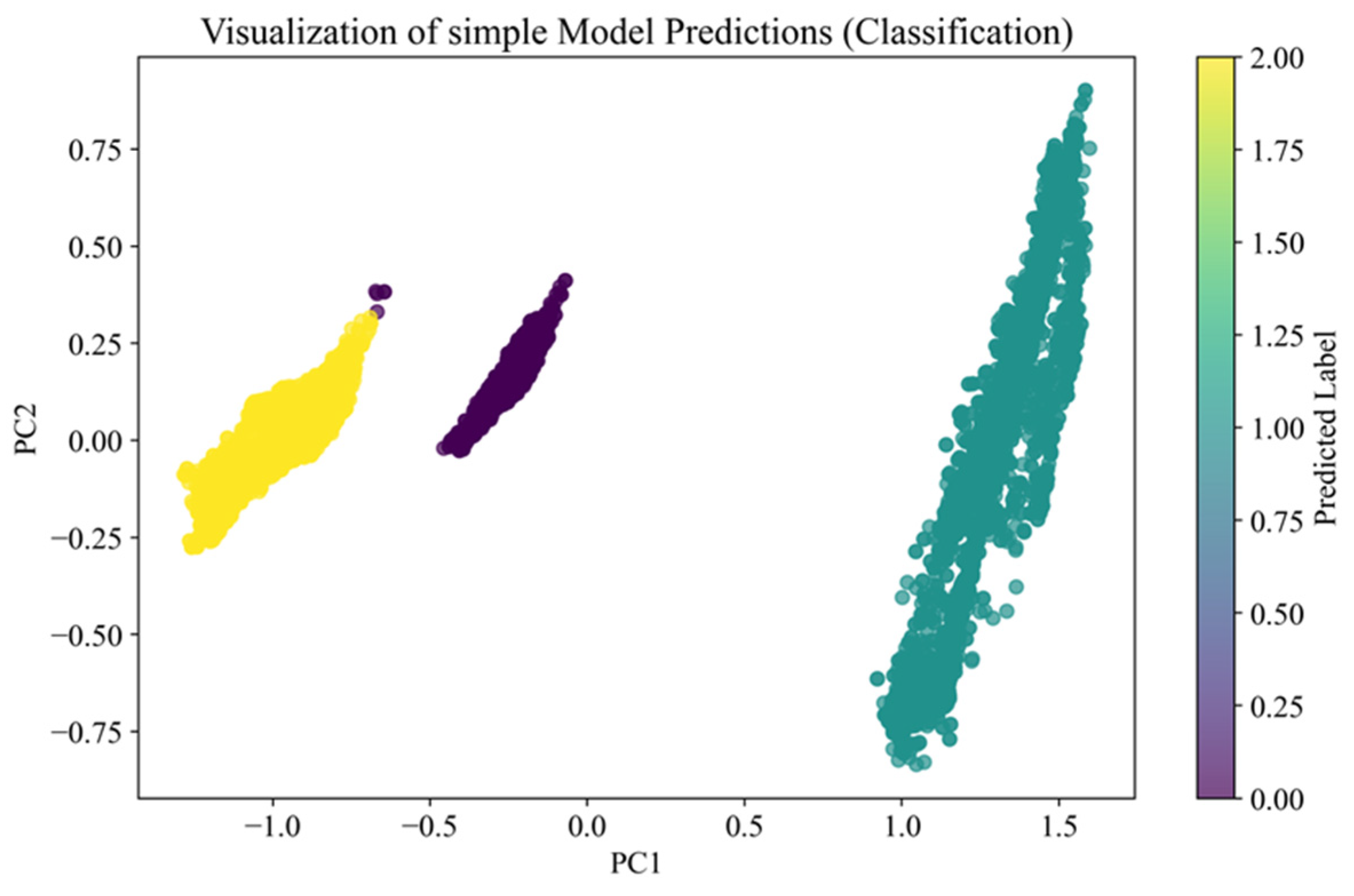
Figure 8 presents the data projected onto the first two principal components (PC1 and PC2), obtained through Principal Component Analysis (PCA). PCA was applied exclusively for visualization purposes, and the first two components explain 97.8% of the total variance, which justifies their use in the diagram. The points are colored according to the predicted labels of the simple model, with each color representing a different class. The visualization reveals that the data are generally grouped into distinct segments; however, some overlap remains between clusters, and not all boundaries are clearly defined. This suggests that while the model can achieve broad separation, it may produce marginal classification errors in cases where spectral feature distributions are insufficiently distinct or overlapping.
Figure 9 visualizes the clustering results. It also uses principal components for a two-dimensional data projection. Still, the final labels were obtained by combining several clustering methods (K-Means, agglomerative clustering, and DBSCAN) and feature enrichment via XGBoost. The graph shows a more precise separation of objects into groups: clusters are located separately, with noticeable gaps between them. This suggests that the proposed approach was able to better account for multidimensional dependencies in the data, which led to a more accurate and robust segmentation.
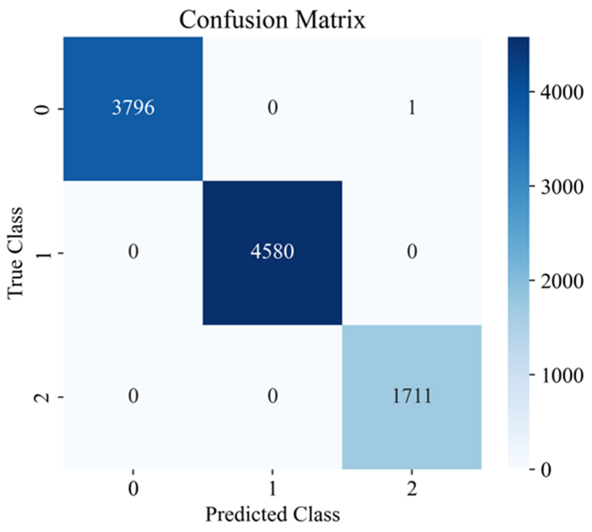
The ensemble model shows a more convincing result in clustering quality and separation clarity. It not only forms well-distinguished clusters but also has a smaller number of borderline objects that are difficult to classify. This is also confirmed by the numerical metrics, which indicate higher Silhouette values and a lower Davies–Bouldin value for the proposed approach. In
Figure 10, the Predicted Class is plotted horizontally, and the True Class is plotted vertically. The numbers inside the cells show how many objects of each actual class (0, 1, or 2) the model assigned to a particular predicted class. It is clear that almost all objects are concentrated on the diagonal: 3796 from class 0 were correctly predicted as 0, 4580 from class 1 as 1, and 1711 from class 2 as 2. The only error is one object of actual class 0, which was erroneously assigned to class 2 (cell in the first row, third column).
Thus, the presented results demonstrate that the proposed model effectively copes with spatial segmentation and quantitative soil salinity assessment, surpassing the baseline model based on the K-Means algorithm in all key metrics. High values of Silhouette Score and ARI, a decrease in Davies–Bouldin Score, and minimal values of MAE and RMSE errors confirm the structural clarity of the clusters and the high accuracy of numerical predictions. PCA data visualization showed that the ensemble model forms more isolated and interpretable groups, consistent with the numerical metrics. The minimum number of classification errors (only one out of more than 10 thousand records) indicates a high reliability of the identified classes. All this confirms that a comprehensive combination of unsupervised methods, probabilistic enrichment, and neural network multi-task learning provides more accurate, robust, and practical results than traditional approaches.
To assess the reliability of the ERA5-Land soil moisture data used in this study, we independently validated the volumetric water content in the topsoil layer (swvl1, 0–7 cm) across the three selected regions. For this purpose, daily soil moisture data from the SMAP L3 passive radar product (spatial resolution 9 km) for 2020–2023 were used as reference. A total of 27 SMAP grid cells overlapping with the study areas were extracted, and statistical comparison with ERA5 values was conducted. The results yielded a mean correlation coefficient of R = 0.71 ± 0.06, a mean bias of −0.016 m
3/m
3, and an RMSE of 0.039 m
3/m
3. These values are consistent with those reported in prior studies (e.g., [
27,
28]) and support using ERA5 data to capture relative soil moisture dynamics. Nevertheless, we acknowledge the need for ground-truth calibration, and a field campaign using TDR sensors is planned for the 2025 season. In addition, although the raw spectral bands from Sentinel-2 provide a comprehensive information base, we found that integrating derived spectral indices (e.g., NDVI, NDSI, BI, SI1–SI5) substantially improves model performance. These indices are physically meaningful transformations that enhance contrast between soil types (e.g., salty crusts, vegetation, and sand). Control experiments showed that using only the 13 original bands reduced the F1-score from 0.999 to 0.987, while including indices restored the original performance. Furthermore, normalized indices improve noise resistance, reducing feature variance by up to 20%, and are readily available or computable in real-time from platforms such as Google Earth Engine and Sentinel Hub. Thus, their use ensures higher accuracy and consistency between training and operational deployment of the model.
Limitations and Future Work
Despite the promising results, the proposed methodology has several limitations that should be acknowledged. First, the model exhibits sensitivity to atmospheric scattering under high aerosol concentrations, which may affect spectral index accuracy. Second, during periods of dense vegetation cover, the contrast of key indices (e.g., NDVI, NDWI) may decrease, reducing segmentation performance. Third, the spatial resolution of climate covariates from the ERA5-Land dataset remains relatively coarse, potentially limiting local-scale precision. Fourth, the model was primarily trained and validated in arid and semi-arid regions, so its transferability to humid or highland zones requires further testing. Fifth, ground-truth data on electrical conductivity are incomplete, and field calibration campaigns are planned to address this gap.
To enhance the robustness and generalizability of the method, future work will focus on several directions:
Integrating synthetic aperture radar (SAR) data to improve sensitivity to soil moisture;
Adopting deep segmentation architectures such as U-Net for finer pixel-level classification;
Incorporating season-aware mechanisms to adapt model performance across different phenological phases.


 ,
, 

