Abstract
The density-based spatial clustering of applications with noise (DBSCAN) is able to cluster arbitrarily structured datasets. However, the clustering result of this algorithm is exceptionally sensitive to the neighborhood radius (Eps) and noise points, and it is hard to obtain the best result quickly and accurately with it. To address this issue, a parameter-adaptive DBSCAN clustering algorithm based on the Sparrow Search Algorithm (SSA), referred to as SSA-DBSCAN, is proposed. This method leverages the local fast search ability of SSA, using the optimal number of clusters and the silhouette coefficient of the dataset as the objective functions to iteratively optimize and select the two input parameters of DBSCAN. This avoids the adverse impact of manually inputting parameters, enabling adaptive clustering with DBSCAN. Experiments on typical synthetic datasets, UCI (University of California, Irvine) real-world datasets, and image segmentation tasks have validated the effectiveness of the SSA-DBSCAN algorithm. Comparative analysis with DBSCAN and other related optimization algorithms demonstrates the clustering performance of SSA-DBSCAN.
1. Introduction
Data mining denotes the process of extracting valuable knowledge and information from large datasets, with the aim of uncovering useful information hidden within the data. Clustering analysis is one of the important research directions in data mining and has applications in fields such as face recognition, image analysis, inventory forecasting, medical image processing, and text analysis [1,2,3,4]. DBSCAN [5] is a classic density-based clustering algorithm that divides high-density regions into clusters and performs clustering in datasets with noise, allowing for arbitrary-shaped clusters. However, this algorithm has two drawbacks: first, it requires the manual specification of the parameters Eps and MinPts without prior knowledge; second, the choice of Eps and MinPts is crucial. Usually, the selection of MinPts parameters is greater than or equal to the data dimension plus one, and then the appropriate Eps is found through the k-distance graph, that is, the “inflection point” of the k-th nearest neighbor distance is identified as the candidate radius. Improper settings may lead to incorrect clustering results or even failure to cluster at all. To address the limitations of the DBSCAN algorithm, various scholars have proposed different solutions, among which parameter adaptation is a commonly used approach. Lu et al. [6] improved DBSCAN based on the gray relational matrix (SAG-DBSCAN), which divides the dataset into dense and sparse subsets through local density measurement and clusters the dense parts using DBSCAN. Cao et al. [7] proposed an improved density clustering method by combining the particle swarm optimization (PSO) algorithm with DBSCAN. PSO automatically searches for the optimal combination of neighborhood radius (Eps) and minimum sample size (MinPts) parameters to enhance the robustness and clustering effect of the traditional DBSCAN algorithm to parameter sensitivity. Li et al. [8] proposed an improved density clustering algorithm based on the nearest neighbor graph (NNG). The core idea is to directly identify local high-density samples by analyzing the inherent properties of the nearest neighbor graph and combine statistical methods to filter noise, ultimately adopting a clustering process similar to the DBSCAN algorithm. Wang et al. [9] proposed an optimization algorithm based on density clustering whose core innovation lies in the polynomial fitting and candidate parameter screening mechanism of k-dist graph, which is combined with a mathematical expectation method and contour coefficient verification to achieve dual parameter adaptive determination of Eps and MinPts, significantly improving the robustness of traditional DBSCAN to parameter sensitivity. Li et al. [10] introduced an improved density clustering algorithm that combines graph neural networks (GNNs) and the DBSCAN algorithm. The core idea is to learn high-order neighborhood relationships between data points through GNNs, dynamically generate neighborhood density thresholds (such as replacing the traditional fixed parameter Eps), and optimize cluster boundary partitioning using graph structure information, thereby improving adaptability to complex topological data. Sunita et al. [11] proposed an improved DBSCAN algorithm that combines the k-nearest neighbor (KNN) concept. Its core innovation lies in dynamically adjusting the local neighborhood density threshold using the k-nearest neighbor distance, replacing the fixed global parameter Eps of traditional DBSCAN, thereby enhancing its adaptability to data with uneven density. This algorithm typically generates candidate neighborhood radii automatically by constructing a KNN distance map and combines statistical methods to screen for the optimal parameter combination, achieving more robust clustering. Bryant et al. [12] proposed RNN-DBSCAN, which is an improved density clustering algorithm based on reverse nearest neighbor (RNN) density estimation. By using k-nearest neighbor graph traversal instead of fixed radius neighborhood search in the traditional DBSCAN algorithm, the algorithm parameters are simplified to only select k values and the ability to handle density non-uniform datasets is enhanced. Li et al. [13] proposed an improved DBSCAN algorithm based on dynamic adjustment of neighborhood density using k-nearest neighbors. The core idea is to adaptively generate local density thresholds by calculating the k-nearest neighbor distance distribution of each data point, replacing the fixed global parameter neighborhood radius (Eps) of the traditional DBSCAN algorithm, thereby improving the clustering robustness of data with uneven density. Li et al. [14] proposed an innovative clustering method called partition KMNN-DBSCAN, aimed at solving the parameter setting problem of the traditional DBSCAN algorithm when dealing with data with uneven density or high noise. Firstly, the K-median nearest neighbor method was used to preliminarily partition the data, reducing the uncertainty of DBSCAN parameter selection and making the clustering effect more stable. However, even so, when dealing with large-scale or complex datasets, a single global clustering strategy may still face difficulties. Therefore, partition KMNN-DBSCAN further preprocesses the data by introducing a “partition” strategy, dividing the entire dataset into several subregions, with data in each subregion having a more uniform density distribution, and clustering separately based on the local features of each subregion. This partitioning method ensures that each local data subset can obtain more suitable ε and MinPts parameters, thereby improving the accuracy and efficiency of clustering. In each partition, partition KMNN-DBSCAN combines adaptive parameter selection by locally optimizing the parameters of each subset, ensuring that the most suitable clustering parameters can be automatically selected based on the density characteristics of local data. During the optimization process, the algorithm dynamically adjusts parameters by evaluating the clustering effect, making the final clustering results more in line with the actual distribution characteristics of the data. The partition clustering results will eventually be integrated into a complete global clustering structure, ensuring the completeness and accuracy of the final clustering. Zhou et al. [15] introduced an improved adaptive density clustering algorithm (AF-DBSCAN), whose core innovation lies in fitting inflection points based on k-dist curve statistical distribution characteristics to adaptively select global parameters Eps and MinPts while reducing redundant calculations by optimizing regional query strategies, thereby improving the efficiency and parameter robustness of traditional DBSCAN. Chen et al. [16] introduced a density clustering algorithm for optimizing wafer manufacturing data. Its core innovation lies in combining spatial indexing to accelerate neighborhood search and improving the clustering accuracy of wafer surface temperature or defect distribution maps through adaptive parameter selection and data dimensionality reduction preprocessing, thereby optimizing anomaly detection and quality control in the wafer manufacturing process. Juan et al. [17] introduced an improved density clustering method that optimizes DBSCAN parameters or clustering process through genetic algorithm (GA), using factor analysis to group data. Its core objective is to solve the sensitivity of traditional DBSCAN to parameters through a global search strategy and improve adaptability to complex data distributions. Zhang et al. [18] proposed an improved DBSCAN density clustering method based on the Whale Optimization Algorithm (WOA). Its core innovation lies in utilizing the global search capability of WOA to adaptively optimize the neighborhood radius Eps and minimum sample size MinPts of DBSCAN algorithm. By simulating whale predation behavior through the “enclosure—bubble network attack—search” strategy, the exploration and development capabilities of parameter search are balanced, thereby improving the clustering robustness of data with uneven density. Wang et al. [19] introduced AMD-DBSCAN, which employs the variance of neighborhood numbers to quantify the density variation across clusters. This approach requires only a single hyperparameter, minimizing redundant computations and demonstrating superior performance on datasets with varying density distributions. Yang et al. [20] proposed a novel clustering algorithm OBLAOA-DBSCAN, which effectively solves the problem of the traditional DBSCAN algorithm being sensitive to parameters and finding it difficult to automatically determine core parameters, such as neighborhood radius Eps and minimum number of neighbors MinPts when processing complex data, by combining arithmetic optimization algorithm (AOA) with the inverse learning strategy (OBL). The algorithm first utilizes the OBL to improve the diversity of the initial population and the coverage of the search space. Then, through the powerful arithmetic-driven search mechanism of AOA, the parameter combination of DBSCAN is continuously optimized during the iteration process, resulting in significant improvements in accuracy, robustness, and adaptability in the final clustering results. These above methods for optimizing the DBSCAN algorithm have achieved relatively good results, but they still have some shortcomings and challenges. For example, the use of KNN or RNN may lead to different clustering results depending on the value of k. KNN selects the distance at the inflection point as the Eps of DBSCAN by drawing the distance map of the k-th nearest neighbor, where usually k is set as the data dimension plus one. RNN is usually set based on time-series characteristics and selects appropriate values through experiments or visual analysis. Therefore, determining the appropriate k value is a topic that requires further research. In addition, setting MinPts parameters is also quite tricky, and currently most methods can only indirectly determine them through mathematical mapping or heuristic rules, lacking sufficient flexibility. Furthermore, k-nearest neighbor methods and metaheuristic algorithms have shortcomings in terms of computational complexity and convergence speed, which is particularly evident in scenarios involving large-scale data processing or real-time response. Some methods also have strong dependence on initial parameters, lack unified evaluation criteria, and poor adaptability to high-dimensional data. These factors collectively limit the algorithm’s generalization ability and actual deployment effectiveness. Therefore, further improvements are still needed for DBSCAN and its optimization methods to achieve more efficient, robust, and adaptive clustering effects.
Metaheuristic algorithms optimize complex problems by mimicking certain behaviors found in natural and social systems. The Sparrow Search Algorithm (SSA), proposed by Xue [21], is a new metaheuristic algorithm that finds the optimal point by simulating the predation and anti-predation behaviors of sparrows. Due to the Sparrow Search Algorithm’s few parameters and strong global search capabilities, this paper proposes an improved adaptive DBSCAN algorithm based on the Sparrow Search Algorithm (SSA-DBSCAN) which combines the rapid convergence and robust optimization performance of the Sparrow Search Algorithm (SSA) to dynamically adjust DBSCAN’s parameters. The silhouette coefficient serves as the fitness function within the SSA framework, enabling the algorithm to identify the optimal cluster quantity and maintain high clustering quality. The result is a fully adaptive DBSCAN clustering process that does not require input parameters, offering advantages such as simplicity and high accuracy in clustering results.
This paper aims to clearly explain the core principles of the algorithm, provide a comprehensive overview of SSA-DBSCAN, conduct experimental analyses, and present conclusions.
The contributions of this paper are as follows:
- (1)
- Combining Sparrow Search Algorithm with DBSCAN to improve the efficiency of the latter.
- (2)
- The proposed algorithm underwent testing on five artificial datasets, seven real-world datasets, and five real images, showing strong performance with low- and medium-dimensional real data.
- (3)
- Improved the parameter selection process of DBSCAN algorithm.
- (4)
- Reducing the loss of flexibility in the current adaptive DBSCAN method helps to effectively maintain clustering quality.
The remainder of this paper is structured as follows. Section 2 presents the fundamental principles and operational procedures of both the DBSCAN algorithm and the Sparrow Search Algorithm (SSA). Section 3 elaborates on the design and implementation of the proposed SSA-DBSCAN approach. In Section 4, an experimental evaluation is described, focusing on the performance of SSA-DBSCAN across synthetic datasets, benchmark datasets, and real-world image data. The outcomes are compared with those of several widely used clustering techniques, followed by an in-depth discussion. Section 5 offers a summary of the experimental findings along with a sensitivity analysis. Lastly, Section 6 concludes the study and outlines potential directions for future work.
2. DBSCAN Algorithm and Sparrow Search Algorithm
2.1. DBSCAN Algorithm
The DBSCAN algorithm is a density-based clustering algorithm introduced by Martin Ester et al. [5] in 1996. The core idea is to use the density connectivity to divide regions that are density-connected into a single cluster, while marking noise points as those that do not belong to any cluster. Therefore, this algorithm can discover clusters of arbitrary shape and is robust to outliers.
The DBSCAN algorithm begins by randomly selecting an unvisited data point. It then examines whether enough points lie within the neighborhood of this point, defined by a radius Eps. Specifically, it checks if there are at least MinPts points within that area. When this condition is met, it marks the point as the core point, creates a new cluster, and recursively expands it: adding all unvisited points in the neighborhood of the core point to the candidate set. If the candidate points also meet the core point conditions, neighborhood is expanded to form clusters with direct density, reachable density, or connected density. If there are not enough neighboring points, the point is temporarily classified as noise and may be absorbed as a boundary point by clusters of neighboring core points in the future. All unclassified points are ultimately considered noise, while boundary points are assigned based on the cluster of core points they belong to. Upon completion of processing all points within a cluster, the algorithm moves on to the next unvisited point. This cycle continues until every data point is assigned to a cluster or marked as noise. Through this process, DBSCAN effectively identifies clusters of varying shapes and demonstrates some resilience to noise. The detailed steps of the DBSCAN algorithm are as follows:
Step 1: Input the dataset, neighborhood distance value Eps, and neighborhood density threshold MinPts.
Step 2: Traverse all sample points. Search for core sample points based on Eps and MinPts and add the core sample points to the core sample set.
Step 3: Select a core sample point and find its density-connected sample points to form a cluster.
Step 4: Find new core sample points and repeat Step 3.
Step 5: Mark any sample points not included in any cluster as noise points.
2.2. Sparrow Search Algorithm
Sparrow Search Algorithm is a completely new metaheuristic algorithm. Suppose the sparrow population consists of n sparrows. Equation (1) outlines the sparrow population as follows:
where n refers to the number of sparrows in the group, while d indicates how many dimensions the optimization task involves. Equation (2) outlines how the discoverer’s position is updated, and it is as follows:
where t stands for the current iteration. j refers to the dimension where j ranges from 1 up to d. denotes a constant that sets the upper limit for iterations. shows the spot of the i-th sparrow in the j-th dimension. A random number appears as . The term reflects the warning threshold, while means the safe threshold. Q stands for a random value drawn from a normal distribution. L describes a matrix filled entirely with ones. When , it indicates that the foraging environment is relatively safe, and the discoverer’s search range is relatively large. When , it indicates that a predator has been discovered, and all sparrows need to fly to other safe areas for foraging. Equation (3) outlines how the follower’s position is updated, and it is as follows:
where i denotes the number of joiners, n refers to the total number of sparrows, shows the best position the discoverer holds now, marks the global worst spot at this moment, and A stands as a matrix filled with either 1 or −1, and . When , it is equivalent to the sparrow being in a state of hunger and needing to move to other areas to find more food. During the foraging process, a few sparrows act as sentinels and SD sparrows are randomly selected from the population as watchers in each generation. Equation (4) outlines as follows how the sentinel’s position is updated:
where refers to the best position found so far across the entire population. acts as a parameter managing the step length, chosen from a normal distribution with a mean of zero and a variance of one. serves as another random number that influences both the step size and the movement direction of sparrows. gives the fitness value for the current sparrow. and denote the current highest and lowest fitness values among all individuals. is a small constant to avoid division by zero in the denominator.
3. Improved DBSCAN Algorithm Based on Sparrow Search Algorithm
3.1. Basic Idea
The DBSCAN algorithm can identify clusters of arbitrary shapes and effectively handle outliers. However, the algorithm’s efficacy is substantially shaped by the chosen parameters, namely Eps and MinPts, which often require a lot of anthropogenic experimentation to determine. This manual tuning typically involves extensive experimentation. Moreover, for different datasets, the DBSCAN algorithm requires different Eps and MinPts parameters, which limits its applicability.
To solve this problem, the number of clusters in the dataset is automatically determined by the density peak. Utilizing the local fast search capability of Sparrow Search Algorithm, combined with contour coefficient as fitness function, iteratively selecting the optimal solution of the two input parameters of DBSCAN to avoid the adverse effects of manual input parameters on clustering results, thus finding the best clustering solution and achieving adaptive clustering of SSA-DBSCAN.
3.2. Determine the Parameter Range and the Optimal Number of Clusters
3.2.1. Adaptive Calculation of Parameter Ranges
In the SSA-DBCSAN algorithm, the parameter Eps depends on how the sample points are distributed within the dataset. The key steps are outlined below:
Step 1: Start by creating the distance distribution matrix for dataset D using the following equation:
where represents the matrix is symmetric, n represents the count of items in dataset D, and is denoted as the distance between the i-th and j-th object in dataset D.
Step 2: For each row in the distance matrix , sort the distances in increasing order. The first column will always be zero, since every object has zero distance from itself. By looking at the sorted k-th column, we can create a distance vector that collects the distance of each object to its k-th nearest neighbor.
Step 3: Find the average value in this k-nearest neighbor distance vector , which is the k-average nearest neighbor distance , which can also be considered as a possible value for the Eps parameter. By repeating this for different k values, we can build a list of candidate Eps parameters, which is denoted as follows:
Step 4: Obtain each value from the list of Eps parameters, and for each object in the dataset count how many other objects fall within that Eps distance. Then, calculate the mathematical expectation of these counts for all objects. This will become the MinPts parameter, which will be used as the threshold for the neighborhood density in dataset D, which is denoted as follows:
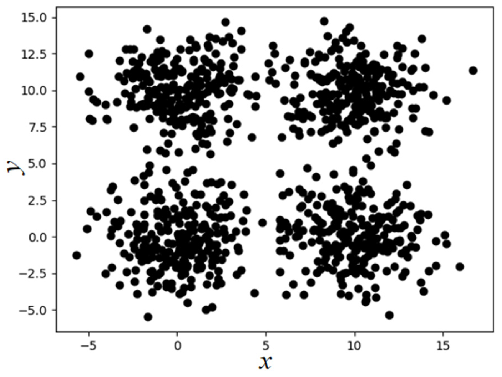
where represents the number of objects in the Eps neighborhood of the i-th object, and n represents the total number of objects in the dataset D. This paper takes the SampleD dataset as an example (the distribution of sample points is shown in Figure 1, which contains a total of 2000 sample points from four categories). Following the above steps, the maximum value of is 19.82. Therefore, the Eps parameter range of the SampleD dataset is , and the MinPts parameter range is .
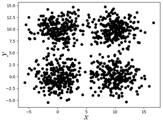
Figure 1.
Two-dimensional display of SampleD dataset.
3.2.2. Determine the Optimal Number of Clusters
Analysis of global data through kernel density estimation can only roughly determine the sparsity of the dataset, but local density analysis can calculate the appropriate number of clusters in the dataset [22]. The DPC algorithm [23] leverages such characteristics to determine cluster centers. However, the DPC algorithm still requires manually specifying a truncation distance , and the final selection of cluster centers is performed through observation. In this paper, the bandwidth parameter is used to adaptively select the truncation distance, and the clustering centers are determined by analyzing the slope between sample points in the decision diagram, comparing the distances between suspected center points. The specific steps are as follows:
In the given dataset D, randomly select a point g. The following two values can be defined: denotes local density and refers to the distance to the point with a higher local density. The local density can be defined as follows:
where represents the distance between two points and is the truncation distance [24].
If the subscript arrangement of the data point local density is expressed as , satisfying , then the distance from point g to the point with a higher local density can be defined as follows:
Each sample point in dataset D is abstractly represented by . To more accurately ascertain the optimal cluster quantity, the influence of and is taken into account to define . Greater values suggest a higher probability of representing the cluster’s center [25]. organizes into a sequence where each value is less than its predecessor. p represents the point with the greatest degree of change between and , and the point p satisfies the following:
where symbolizes the slope between successive data points, while and denote the mean and aggregate discrepancies in these slopes, respectively. On this basis, this paper theoretically achieves automatic determination of the number of clustering clusters. By analyzing the trend of value changes, calculating the slope of adjacent points, and searching for “mutation points”, the boundary between representative clustering centers and ordinary points can be determined. This mutation point reflects the number of significant density peaks in the data and is the theoretical basis for estimating the number of cluster centers. In addition, establishing the ultimate cluster quantity is also influenced by factors such as the structure of the data itself, bandwidth parameters, and the selection method of truncation distance . Specifically, the distance relationship between density centers is also used to eliminate “pseudo centers” that are too close in high-density regions, further improving the accuracy and stability of clustering structure recognition.
The inherent distribution structure of data, the selection of bandwidth parameters, the determination of truncation distance , and the spatial relationships between suspected cluster centers all have an impact on the optimal cluster quantity. A suspected clustering center can be defined as follows:
According to the nature of the density peak algorithm, the real clustering centers are generally distributed in the areas with higher density compared to other regions, and the relative distance between the centers is relatively far. If there are multiple suspected clustering centers in a high-density area, they will usually be in close proximity. Therefore, the shortest distance between the maximum value and the remaining points is judged in turn, that it is not the cluster center if it is less than , and that it is the cluster center if it is greater than .
3.3. Fitness Function Selection
In the case that the real classification label is unknown, the quality of clustering can be described by internal metrics, and calculating the contour coefficient is a commonly used internal cluster measurement method which evaluates the similarity of a sample point with its own cluster rather than other clusters. The specific formula is defined as follows:
where denotes the mean proximity of the i-th entity to its fellow members within its cluster. Conversely, signifies the mean proximity of the i-th entity to entities residing outside its own cluster, encompassing all other clusters. Values nearing 1 in the silhouette coefficient denote superior quality in cluster formation.
The contour coefficient is used in Sparrow Search Algorithm as a fitness function and serves as an important indicator to measure the clustering effect because it does not need to calculate the density and dispersion between clusters without specifying the clustering center, and has robustness. Compared with other indicators such as DBI and CH, the silhouette coefficient index is the most widely used indicator. It is possible to evaluate datasets containing various shapes, and the comprehensive effect is optimal. By using this feature of the profile coefficient, the optimal values of Eps and MinPts parameters in DBSCAN can be calculated.
3.4. Iterative Process of Parameter Optimization
By simulating the foraging behavior of sparrows, the parameters Eps and MinPts of the DBSCAN algorithm were optimized. These parameters are represented as the position of a single sparrow. In each iteration, determine the coordinates of the optimal solution and set the range of these coordinates according to the method outlined in Section 3.2.1.
The Sparrow Search Algorithm simulates behaviors such as foraging and evading predators. Discoverers are responsible for finding food for the entire group and providing information about the food’s location and the surrounding area. Followers continuously monitor the behavior of the discoverers and immediately follow and snatch the food once the discoverers locate it. Additionally, sparrows can flexibly switch roles between discoverers and predators. Sparrows in the center of the group sometimes move closer to nearby sparrows to reduce their exposure to danger.
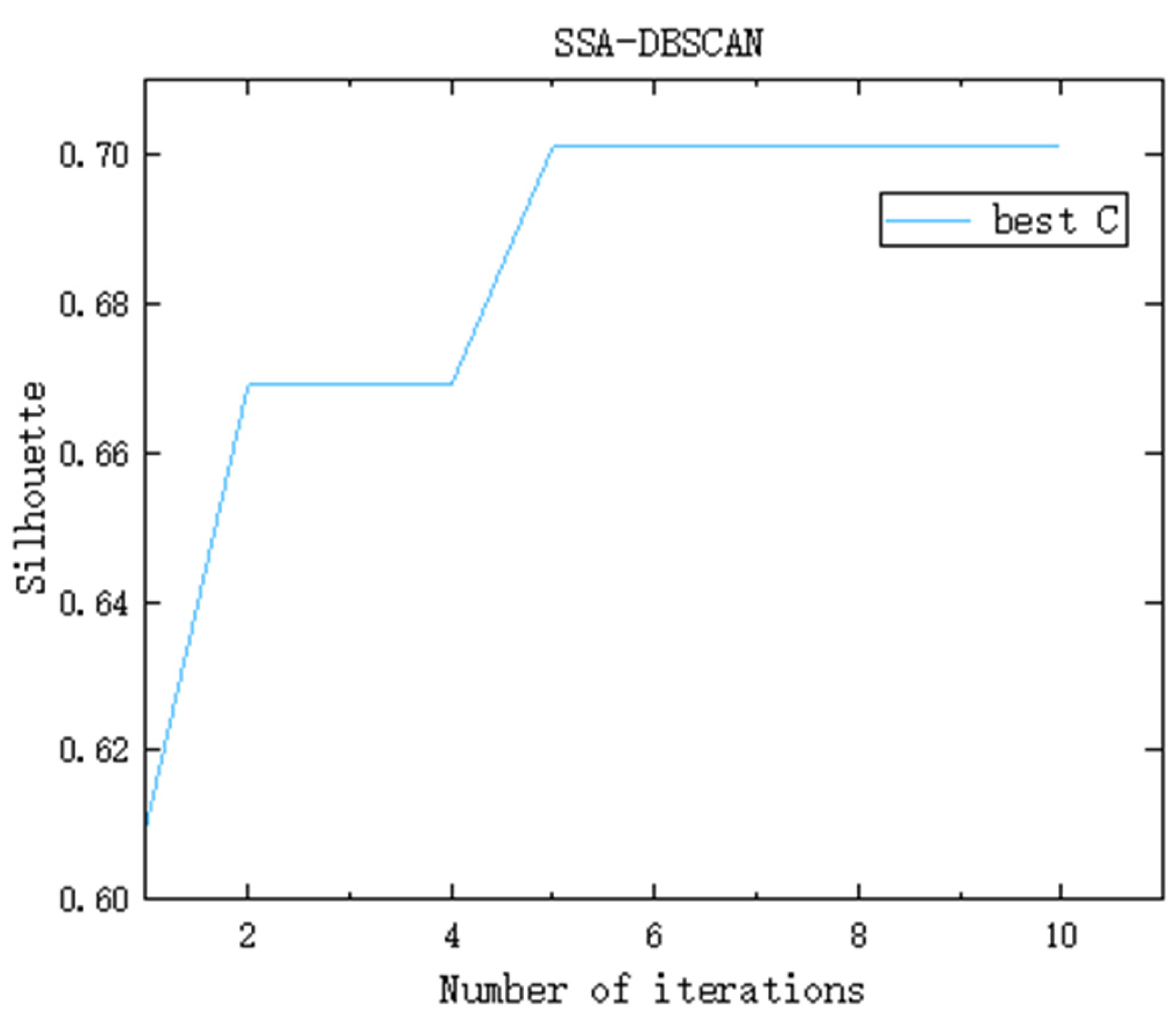
Observers are responsible for monitoring the surroundings of the foraging area. When a predator is detected, observers immediately issue a warning. If the warning signal exceeds the alert threshold, the entire group will quickly move to a new foraging site under the guidance of the discoverers. Taking the dataset SampleD as an example, the DBSCAN parameters Eps and MinPts are optimized through the Sparrow Search Algorithm. The number of randomly generated sparrow individuals is set to 500, and the number of iterations is 10. The evolution of the fitness function over successive iterations is illustrated in Figure 2. Following the fourth iteration, the fitness value of the best solution converges and remains stable at 0.701. At this point, the corresponding optimal parameters for Eps and MinPts are 2.8014 and 79, respectively. Therefore, the SSA-DBSCAN algorithm is capable of adaptively tuning DBSCAN parameters by leveraging the underlying distribution characteristics of the dataset.
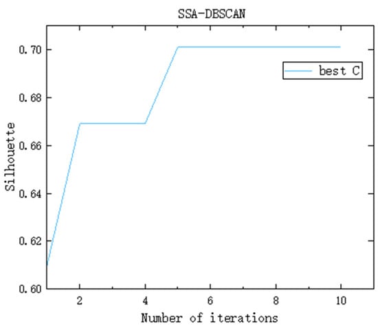
Figure 2.
Iterative change graph of optimal fitness function value (taking the dataset SampleD as an example).
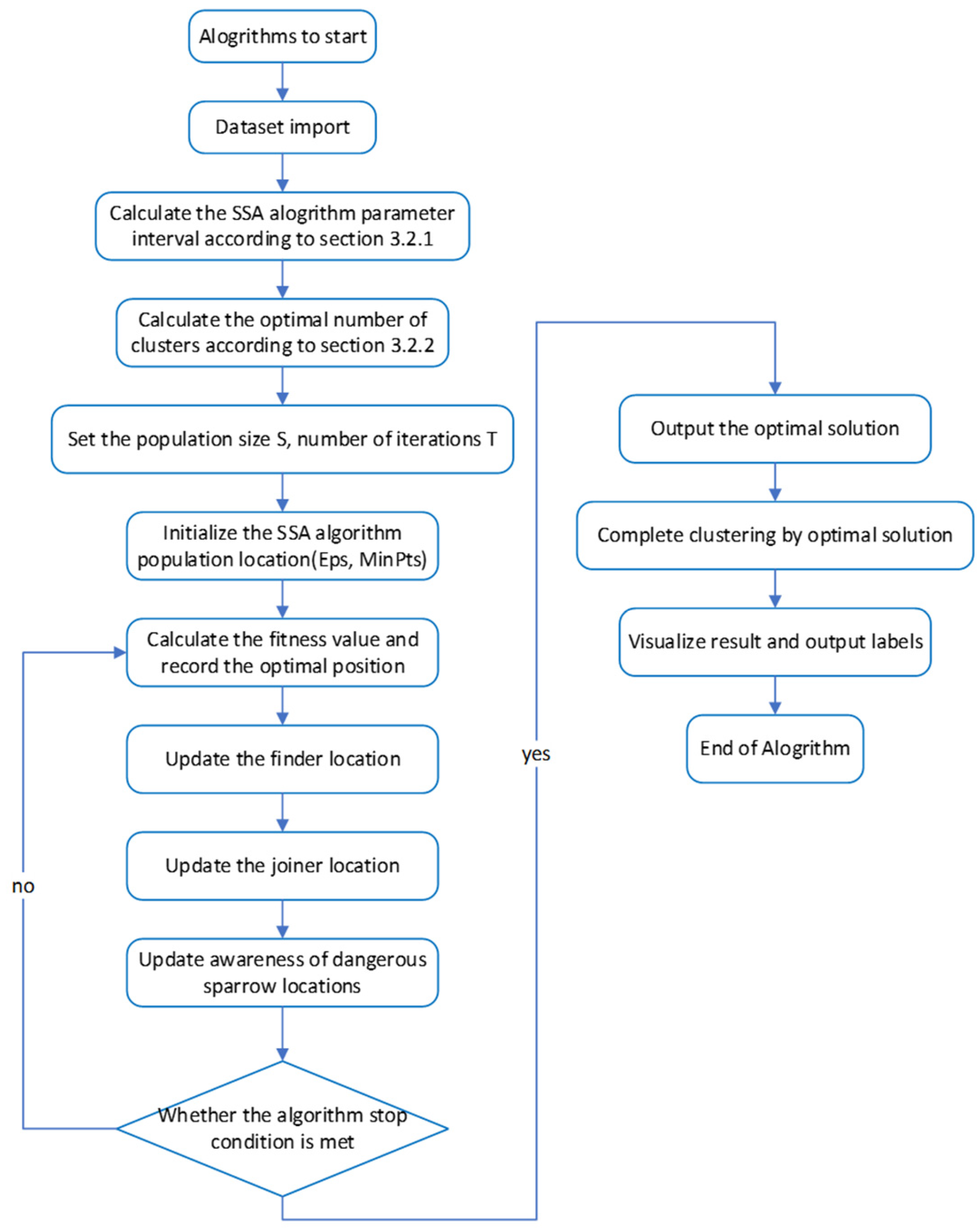
3.5. Algorithm Pseudocode and Flowchart
The key to the SSA-DBSCAN algorithm lies in choosing the optimal cluster quantity, the screening of the optimal solutions during execution, and the latter iterative solution process. The prior knowledge requirement for the dataset is less and the results are more accurate. Algorithm 1 presents the pseudocode for the SSA-DBSCAN algorithm, while Figure 3 illustrates its execution steps.
| Algorithm 1: SSA-DBSCAN | |
| Input: Sample set , Population Size S, Number of iterations T; | |
| 1: | Calculate the distance matrix for dataset D; |
| 2: | Calculation the median of each column in D* ; |
| 3: | Get the range of Eps values ; |
| 4: | Get the range of MinPts values ; |
| 5: | Calculate the local density and the sample point distance , Determine the number of clusters based on the |
| distance relationship ; | |
| 6: | Generate list of sparrow parameters based on Eps and MinPts; |
| 7: | While (t < T); |
| 8: | Obtain the profile coefficient value s(i) of an individual sparrow with the number of cluster n; |
| 9: | The solution that matches the number of clusters and has the largest Silhouette is the optimal solution; |
| 10: | Rank the fitness values and find the current best individual and the current worst individual; |
| 11: | R2 = rand (1) |
| 12: | for i = 1: PD |
| 13: | Using Equation (2) update the sparrow’s location; |
| 14: | end for |
| 15: | for i = (PD + 1): n |
| 16: | Using Equation (3) update the sparrow’s location; |
| 17: | end for |
| 18: | for l = 1: SD |
| 19: | Using Equation (4) update the sparrow’s location; |
| 20: | end for |
| 21: | Get the current new location; |
| 22: | If the new location is better than before, update it; |
| 23: | t = t + 1 |
| 24: | end while; |
| 25: | Initializing a collection of core objects; |
| 26: | for j = 1,2,3,…,m; |
| 27: | Determine the -neighborhood of sample ; |
| 28: | if ; |
| 29: | Add sample to the set of core objects: ; |
| 30: | end if; |
| 31: | end for; |
| 32: | Initialize the number of clusters: k = 0; |
| 33: | Initialize the set of unvisited samples: ; |
| 34: | ; |
| 35: | Record the current set of unvisited samples: ; |
| 36: | Random selection of a core object , Initializing the queue ; |
| 37: | ; |
| 38: | while ; |
| 39: | Fetch the first sample in the queue q; |
| 40: | if ; |
| 41: | ; |
| 42: | Add the sample in to the queue Q; |
| 43: | ; |
| 44: | end if; |
| 45: | end while; |
| 46: | k= k + 1, Number of clusters generated ; |
| 47: | ; |
| 48: | end while; |
| Output: Cluster division | |
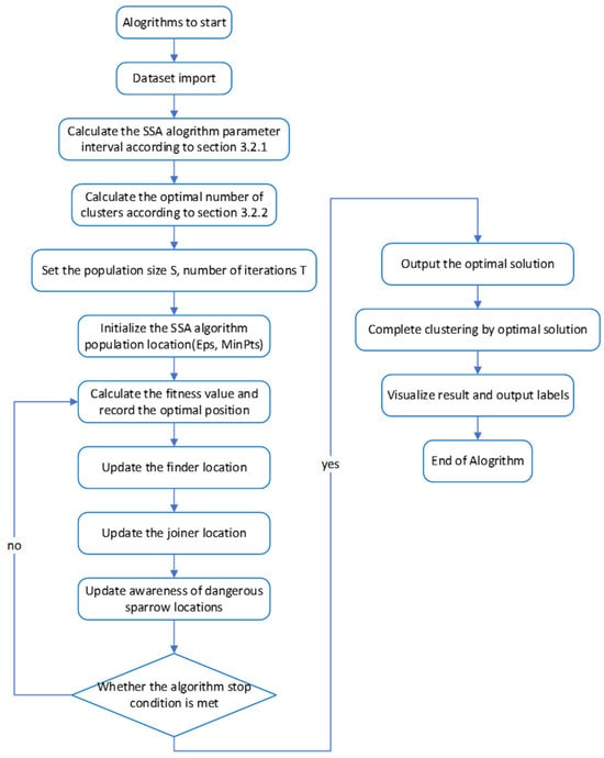
Figure 3.
Core algorithm flowchart.
3.6. Algorithm Complexity Analysis
For a dataset containing n samples, the spatial complexity of DBSCAN primarily arises from assigning cluster labels and categorizing points as core, boundary, or noise. Therefore, the spatial complexity of the DBSCAN algorithm is . In contrast, the integration of the Sparrow Search Algorithm’s iterative optimization process into SSA-DBSCAN leads to an increase in the spatial complexity of the fitness function. Assuming the Sparrow Search Algorithm generates an additional sample size of m, this yields a space complexity of . Consequently, the total spatial complexity of the SSA-DBSCAN algorithm is the overall spatial complexity of SSA-DBSCAN, which is . The time complexity of the SSA-DBSCAN algorithm is mainly determined by the optimization iteration process of the DBSCAN algorithm and sparrow optimization algorithm. For the case where the dataset contains n sample points, the time complexity of DBSCAN largely depends on the duration needed to identify the Eps neighborhood of each sample point and determine its category based on density criteria. In the worst case, the DBSCAN algorithm needs to calculate the distance between each point and all other points, so the time complexity of the DBSCAN algorithm is . The Sparrow Search Algorithm’s time complexity cost is primarily attributed to its iterative optimization procedure and the repeated evaluation of the fitness function across all individuals in the population. The time complexity in the optimization stage is calculated as , given a population size of S and T optimization iterations. The time complexity of the total number of iterations during the iteration process is . The time cost associated with optimizing the fitness function is largely attributed to the calculation of silhouette coefficients. When evaluating the clustering effect, it is necessary to calculate the contour coefficient of each sample point and take the average of the contour coefficients of all sample points to obtain the total contour coefficient. Therefore, the time complexity of the overall contour coefficient is . Accordingly, the total time complexity of the SSA-DBSCAN algorithm is less than .
To sum up, the complexity of the SSA-DBSCAN algorithm is slightly higher than that of the traditional DBSCAN algorithm, but it is consistent in magnitude with the DBSCSN algorithm while ensuring the accuracy of clustering in general scenarios.
4. Experiments and Results Analysis
4.1. Experimental Environment and Comparison Algorithms
The SSA-DBSCAN algorithm was run on a 64-bit Windows 10 system, with hardware specifications including an Intel Core i7-9750H processor, 16 GB of RAM, and a 1 TB hard drive.
In these comparison algorithms, the RNN-DBSCAN [12] algorithm advances the classic DBSCAN framework by leveraging reverse k-nearest neighbor dynamics. By introducing a unified control variable, k, which signifies the count of requisite reverse nearest neighbors, it simplifies the original Eps and MinPts parameters. The process of clustering is then executed through the calibration of the k value. Similarly, the KANN-DBSCAN [13] algorithm applies a nearest neighbor strategy to estimate appropriate parameter values. By computing the average distance to each point’s nearest neighbors, the algorithm estimates Eps and determines MinPts through mathematical expectation. It then constructs a pool of candidate parameters, selecting the combination that yields the highest clustering effectiveness. The AF-DBSCAN [15] algorithm identifies optimal parameters by fitting clustering outcomes using mathematical modeling and selecting the best result through repeated experimentation. The DBSCAN [5] algorithm remains a foundational density-based clustering technique and continues to be one of the most widely adopted methods in the field. In this experiment, the DBSCAN algorithm was optimized through multiple parameter adjustments to obtain the best clustering results based on existing research. The k-means [26] algorithm is a classic partition-based clustering algorithm that requires the user to manually input the number of clusters and iteratively updates the cluster centers to reach the final result. The DPC [23] algorithm is an innovative density-based clustering algorithm that calculates local density and center shift distances, allowing it to find cluster centers in one step without the need for iteration.
4.2. Experimental Datasets and Clustering Evaluation Indicators
To evaluate the overall performance of the SSA-DBSCAN algorithm, five classic synthetic datasets and seven UCI datasets were used for testing. Table 1 provides a summary of the datasets and their key details. The five artificial datasets primarily assess the algorithm’s performance across datasets with varying shapes. The aggregation dataset is a 2D dataset containing seven classes and 788 objects, representing a cluster-connected type of dataset. The compound dataset is a 2D dataset containing six classes and 399 objects, representing a clustered, density-uneven, nested type of dataset. The R15 dataset is a 2D dataset containing 15 classes and 600 objects, representing a density-uniform but non-connected clustered dataset. The spiral dataset is a 2D dataset containing three classes and 312 objects, representing a density-uniform, strip-like similar dataset. The flame dataset is a 2D dataset containing two classes and 240 objects, representing a density-uniform dataset containing two different-shaped clusters.

Table 1.
Experiment datasets.
For the seven real-world datasets, the sym dataset is a visual image dataset obtained from the Waikato Environment for Knowledge Analysis (WEKA) data mining software. The other datasets come from a database proposed by the University of California, Irvine, for machine learning. These datasets cover a wide range of types from artificial synthesis to the real world, with different structural shapes, dimensions, numbers of categories, and task objectives. Clusters such as aggregation, compound, spiral, R15, flame, and sym are 2D synthetic clustering data used to test the recognition ability of clustering algorithms for complex shapes and cluster structures; iris, wine, seeds, and ecoli belong to low- to medium-dimensional real classification data and are suitable for supervised learning model evaluation; zoo and bank contain categorical features, with applications in animal classification and financial marketing prediction, respectively, suitable for classification algorithms; and ecoli class imbalance makes it more suitable for testing the robustness of multi-class classifiers. These datasets have their own characteristics in terms of dimensional complexity, category distribution, visualization friendliness, and preprocessing requirements, and are widely used for algorithm comparison and model validation.
The synthetic data visually demonstrates the clustering performance of different algorithms through graphics. Due to the higher dimensionality of the UCI dataset, we use three evaluation metrics, accuracy (ACC) [27], adjusted mutual information (AMI) [28], and adjusted rand index (ARI) [29], to measure the clustering quality.
The ACC value range is , where values closer to 1 indicate better clustering performance. When ACC > 0.8, it is considered good in most applications; when the ACC value is between 0.6 and 0.8, it indicates moderate performance and whether it is acceptable depends on the application scenario; and when ACC < 0.6, it is usually not ideal unless the task itself is very difficult, or the data are extremely imbalanced.
The AMI value range is . When AMI > 0.5, it indicates that the clustering results are consistent with the true labels; when the AMI value is between 0.3 and 0.5, it indicates moderate and meaningful to some extent; and when AMI < 0.3, it may not make much sense as the clustering results are not consistent with the true labels.
The ARI parameter takes into account the probability of chance, with a range of . Values closer to 1 suggest more accurate clustering results, values closer to 0 suggest that the clustering results are similar to random results, and values closer to −1 indicate that the clustering results are completely opposite to the true categories. When ARI > 0.5, it indicates that the clustering is more consistent with the true category; when the ARI value is between 0.2 and 0.5, it indicates moderate effectiveness; and when ARI < 0.2, it indicates poor performance and clustering may not have practical significance.
To evaluate the clustering performance of SSA-DBSCAN on real images, the probabilistic rand index (PRI) [30] and boundary displacement error (BDE) [31] are used for clustering quality assessment.
The PRI value range is , where a value of 0 indicates that the segmentation result of the test image is completely opposite to the ground truth and a value of 1 indicates that the segmentation results are identical at every pixel pair. When PRI > 0.8, the effect is good, indicating that there is basically no confusion in clustering; when the PRI value is between 0.6 and 0.8, it indicates that the effect is moderate and needs to be judged based on the application scenario; and when PRI < 0.6, it indicates that there are a large number of outliers mixed in the clustering, which may not be ideal.
The BDE value is typically above 1; the lower the metric, the better the image segmentation performance. BDE generally does not have a universal boundary and needs to be considered based on specific tasks and data resolution. Generally speaking, the smaller, the better.
4.3. Analysis of Experimental Results on Synthetic Datasets
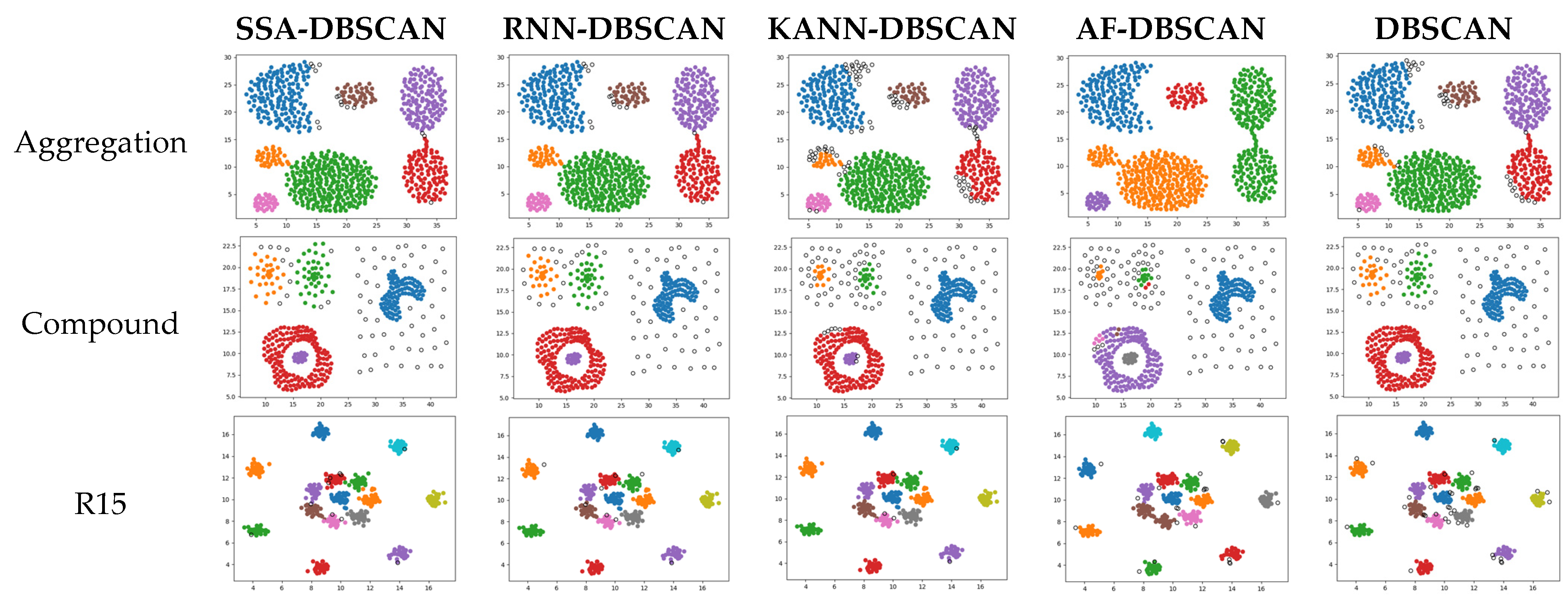
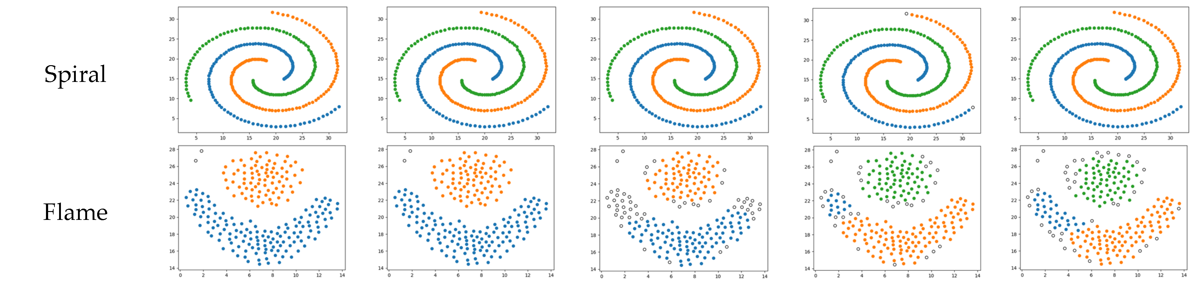
To further verify the effectiveness and advancement of the improved algorithm, cluster analysis was carried out on the artificial dataset and the results obtained by the proposed algorithm were compared with the results of four comparative algorithms. Figure 4 illustrates the performance of different algorithms on various synthetic datasets. Except for the DBSCAN algorithm, the parameters of the other four algorithms can be adaptively calculated. In contrast, the parameters for DBSCAN need to be manually input and optimized.
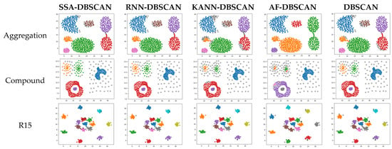
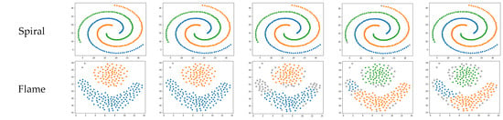
Figure 4.
Clustering results of different algorithms on synthetic datasets.
The aggregation dataset represents a density-homogeneous, cluster-connected dataset. All four algorithms have shown relatively accurate clustering results when clustering this specific dataset. Nevertheless, the AF-DBSCAN algorithm, which adapts parameters through polynomial fitting, can only identify some accurate clusters and fails to effectively separate clusters when they are connected.
The compound dataset exhibits clusters of uneven density and diverse shapes, interspersed with distinct data points. Algorithms such as SSA-DBSCAN, KANN-DBSCAN, and the original DBSCAN can discern these clusters effectively, even though occasional points may be tagged as noise or mislabeled. AF-DBSCAN fails to ensure the effective identification of clusters and is prone to errors, such as misidentifying a single cluster, resulting in the lowest accuracy.
The R15 and spiral datasets comprise uniformly dense, single-shape collections of data. These are datasets in which density-based clustering algorithms perform well. These four algorithms all accurately identify correctly clustered data. However, the KANN-DBSCAN and DBSCAN algorithms mistakenly classify a small number of points as noise, failing to reach the optimal performance. The AF-DBSCAN algorithm experiences a merging of central clusters, which cannot be recognized. On this kind of dataset, all five algorithms perform well, with SSA-DBSCAN yielding optimal performance.
The flame dataset consists of two different shapes of graphics, both of which exhibit uniform density. On this particular dataset, the KANN-DBSCAN algorithm exhibits merely moderate effectiveness despite its commendable results on different collections of data. The AF-DBSCAN algorithm, similar to the KANN-DBSCAN algorithm, mistakenly classifies the clusters as noise. On this type of dataset, the SSA-DBSCAN algorithm outperforms all others, followed by the RNN-DBSCAN and DBSCAN algorithms.
In summary, the SSA-DBSCAN algorithm achieves better clustering results compared to other algorithms that adaptively optimize DBSCAN parameters. For density-uneven datasets with a narrow optimal solution range, it can still perform effective clustering. Therefore, the SSA-DBSCAN algorithm can be applied to more types of datasets, and its accuracy is improved compared to the DBSCAN algorithm.
4.4. UCI Dataset Experiments
Table 2 shows the clustering results of SSA-DBSCAN and four comparative algorithms on UCI real-world datasets, with the best values highlighted in bold.
Table 2.
Comparison of the ACC, AMI, and ARI values across different algorithms (using DBSCAN algorithm as a baseline).
The iris dataset is a 4D dataset consisting of 150 objects in three categories. Based on the evaluation values ACC, AMI, and ARI, both SSA-DBSCAN and AF-DBSCAN achieve good results, with SSA-DBSCAN performing the best, followed by AF-DBSCAN. The other algorithms perform at a similar level.
The wine dataset is a thirteen-dimensional dataset containing 178 objects from three classes. From the perspective of clustering outcome metrics ACC, AMI, and ARI, the RNN-DBSCAN algorithm performs the best, while the second best one is the DBSCAN algorithm. The evaluation indicators for several other algorithms all exceeds 0.6.
The sym dataset is a 2D dataset consisting of 350 objects from three classes. Based on the clustering evaluation metrics ACC, AMI, and ARI, all four algorithms demonstrate good clustering performance. The best-performing algorithm is the SSA-DBSCAN algorithm, while the remaining four algorithms show comparable results.
The seeds dataset is a seven-dimensional dataset containing 210 objects from three classes. According to the clustering metrics ACC, AMI, and ARI, the RNN-DBSCAN algorithm performed the best, while the other four algorithms demonstrated comparable results
The zoo dataset is a sixteen-dimensional dataset consisting of 101 objects from seven classes. Based on the clustering evaluation metrics ACC, AMI, and ARI, the SSA-DBSCAN algorithm demonstrates the best clustering results, while the second best one is the RNN-DBSCAN algorithm. The remaining three algorithms show similar results.
The Bank dataset is a four-dimensional dataset containing 1372 objects from two classes. Based on the clustering evaluation metrics ACC, AMI, and ARI, SSA-DBSCAN achieves the highest performance, with RNN-DBSCAN ranking next. The other three algorithms yield comparable results.
The ecoli dataset is an eight-dimensional dataset with 336 objects from seven classes. According to the evaluation metrics ACC, AMI, and ARI, SSA-DBSCAN provides the best performance, followed by RNN-DBSCAN. The other three algorithms show similar results.
In conclusion, SSA-DBSCAN performs well in clustering multi-dimensional real-world datasets without the need for inputting parameters throughout the process. It outperforms other DBSCAN algorithms with adaptive parameters, showing strong performance on low- and mid-dimensional datasets. However, in high-dimensional datasets, the use of Euclidean distance to calculate sample distances leads to a decline in stability. Moreover, parameter-tuned DBSCAN cannot adapt the parameters based on the clustering results of real datasets; KANN-DBSCAN exhibits anomalous convergence in the number of clusters on high-dimensional datasets; AF-DBSCAN shows poor clustering performance on synthetic datasets; and RNN-DBSCAN demonstrates strong stability with good clustering results.
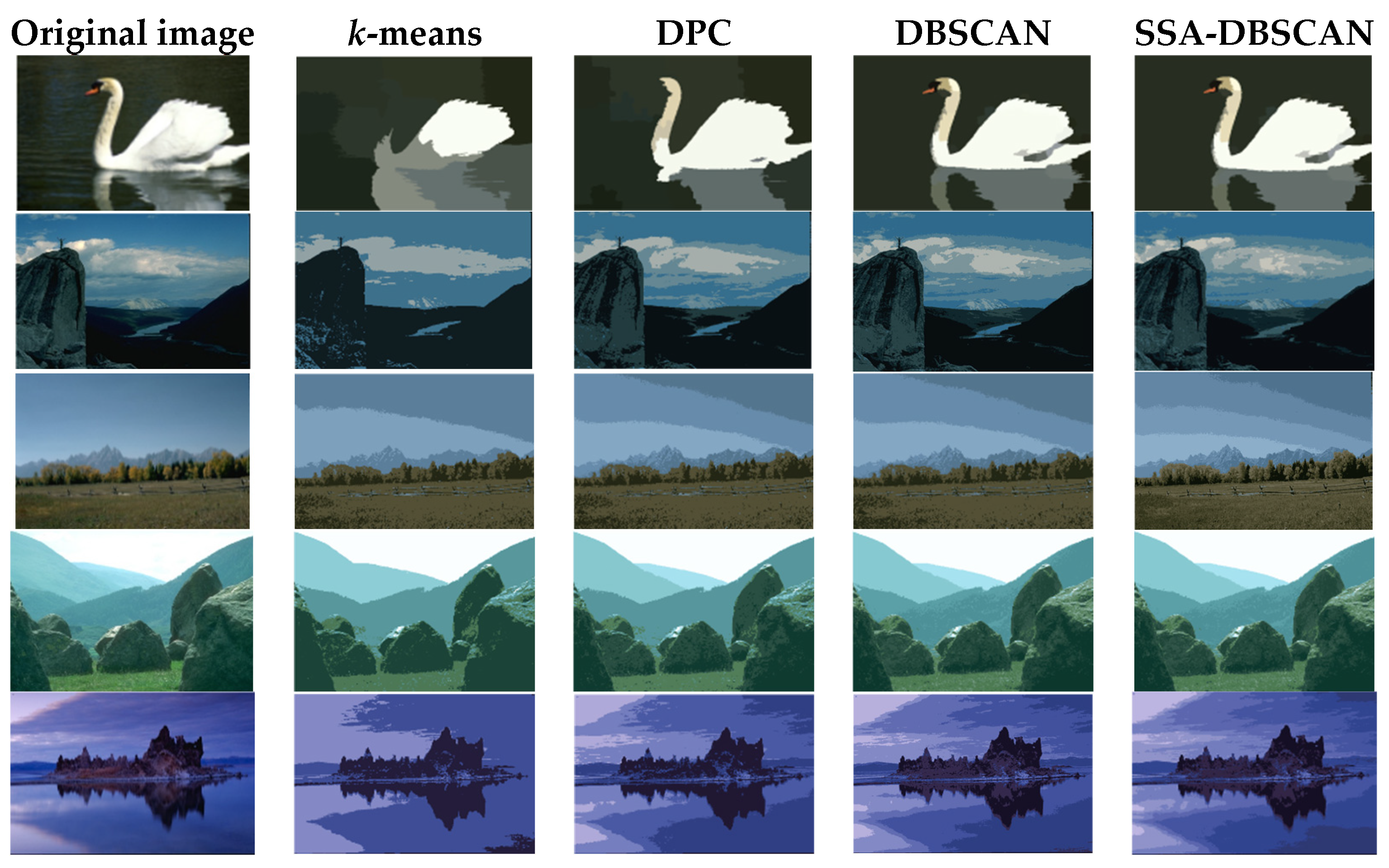
4.5. Image Segmentation
To further verify the performance of SSA-DBSCAN, five real images from the Berkeley Segmentation Dataset (BSDS300) were selected for testing. Figure 5 presents the segmentation results of each algorithm, while Table 3 shows the split metrics of these algorithms.
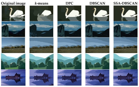
Figure 5.
Image segmentation results of different algorithms.
Table 3.
Comparison of BDE, PRI, running time, and memory size indicators of each algorithm.
To reduce computational volume, we applied the simple linear iterative clustering algorithm to segment images into a collection of super-pixels information prior to their integration into various algorithms.
As we can see from Figure 5 and Table 3, the k-means and DPC algorithms perform poorly in image segmentation compared to other algorithms. Both the DBSCAN and SSA-DBSCAN algorithms are able to segment the image effectively and accurately capture its overall contours. In the second image, the PRI value of the DPC algorithm reaches its maximum value, which is very close to that of the SSA-DBSCAN algorithm. However, SSA-DBSCAN shows a significantly higher BDE value compared to the DPC algorithm. This suggests that the SSA-DBSCAN algorithm performs better than DPC in segmenting the second image.
This can be seen from the data in Table 3 where SSA-DBSCAN’s BDE and PRI values surpass those of DBSCAN, indicating it outperforms in segmenting images with greater precision. Therefore, compared to the other three algorithms, the SSA-DBSCAN algorithm achieves higher segmentation accuracy and produces the best results.
Although the SSA-DBSCAN algorithm provides the best segmentation accuracy, its computational cost is also the highest among the four algorithms. Due to the addition of Sparrow Optimization Algorithm, the SSA-DBSCAN algorithm requires multiple rounds of running DBSCAN, evaluating multiple parameter combinations in each round, resulting in much higher running time and memory usage than other methods. The DPC algorithm relies on a complete point-to-point distance matrix, which requires the calculation of the entire image distance matrix, resulting in high memory consumption and a long running time. The DBSCAN algorithm requires neighborhood search for each point, which involves a lot of distance calculation. The running time and memory increase significantly with the increase in data volume; the k-means algorithm, on the other hand, uses iterative updating of centroids, which results in a linear relationship between computational complexity and data volume. Therefore, it runs the fastest and occupies the least amount of memory.
To sum up, the SSA-DBSCAN algorithm indicates higher accuracy in adaptive parameter search and image segmentation, offering better practicality than the other comparison algorithms.
5. Overview of Experimental Findings and Sensitivity Assessment
5.1. Overview of Experimental Findings
Every object within the datasets yields a definite classification result, which facilitates assessment of cluster efficacy via ACC, AMI, and ARI values. Our proposed SSA-DBSCAN algorithm uses Sparrow Search Algorithm to find the optimal Eps and MinPts values. This approach ensures both rapid convergence and high-quality solutions, leading to strong clustering results on 2D synthetic datasets and several real-world ones.
The experimental results of real images indicate that SSA-DBSCAN consistently achieves superior boundary accuracy and clustering consistency when compared with traditional clustering algorithms such as DBSCAN, k-means, and DPC. Across all evaluated datasets, it outperforms the baselines in terms of clustering quality, as reflected by lower boundary deviation and higher adjusted pairwise similarity. Although SSA-DBSCAN requires greater computational resources in terms of running time and memory usage, the trade-off results in a noticeable gain in clustering effectiveness, particularly in complex or high-variation data scenarios.
The RNN-DBSCAN algorithm exhibits strong performance when applied to synthetic two-dimensional datasets, achieving evaluation scores above 0.9 across all metrics. Nevertheless, since it estimates Eps and MinPts by using reverse nearest neighbor counts it restricts DBSCAN’s clustering capability. Consequently, on certain UCI real-world datasets, DBSCAN variants with extensive parameter tuning surpass its performance.
The KANN-DBSCAN algorithm exhibits strong results on most synthetic datasets but struggles with datasets featuring significant shape variation. Additionally, when tested on high-dimensional real-world datasets, KANN-DBSCAN faces convergence issues with its parameter k.
The AF-DBSCAN algorithm selects optimal parameters by modeling how parameter changes impact the DBSCAN algorithm. Nevertheless, this method demands more stringent dataset conditions and is sensitive to datasets with uneven density distributions.
In our experiments, we tuned the DBSCAN algorithm using a grid search guided by earlier research which attempts to obtain the optimal Eps and MinPts values through manual input repeatedly. While this systematic approach enables exploration of the parameter space, the fixed step sizes may restrict its ability to capture optimal configurations in some datasets. This limitation could lead to a conservative estimate of DBSCAN’s actual clustering potential. Nonetheless, it consistently demonstrates competitive performance in terms of computational efficiency, offering a practical balance between speed and clustering quality.
Overall, the experimental findings underscore the effectiveness of SSA-DBSCAN in achieving high-quality clustering results, particularly when accuracy is prioritized over computational cost. The comparisons affirm the value of intelligent parameter optimization strategies in enhancing DBSCAN-based algorithms for diverse real-world applications.
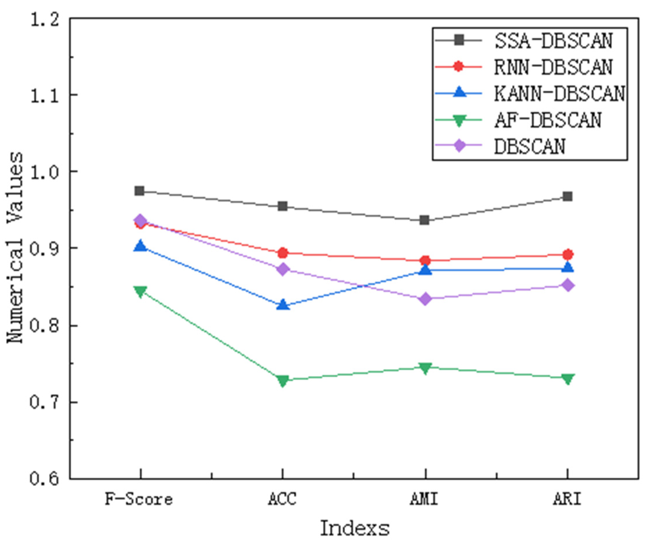
5.2. Sensitivity Assessment
Sensitivity analysis is conducted when there are outliers in the data, mainly to evaluate the potential impact of these outliers on the analysis results and to verify the robustness and reliability of the conclusions. We conducted this analysis using a representative compound dataset, which has multiple outliers in the right-hand region. We compared and analyzed the results of our proposed SSA-DBSCAN algorithm with the other four comparative algorithms using F-Score, ACC, AMI, and ARI.
From the data in Figure 6, we can see that the SSA-DBSCAN algorithm performs the best compared to the other four algorithms on the compound dataset because the Sparrow Search Algorithm can adaptively adjust parameters based on the distribution of outliers, thereby achieving the most stable performance among these indicators. The RNN-DBSCAN algorithm evaluates bidirectional density based on reverse nearest neighbor, but uneven distribution of sparse outliers can lead to bias in core point recognition and cause fluctuations. The KANN-DBSCAN algorithm combines k-nearest neighbors to calculate local density, but density mutations around outliers can amplify local fluctuations and disrupt cluster continuity. The AF-DBSCAN algorithm adopts adaptive filtering in the preprocessing stage, but excessive removal or retention of outliers may damage the true cluster structure. The DBSCAN algorithm relies on static parameters, and although it identifies noise through density thresholds, fixing Eps and MinPts may lead to misjudging cluster boundaries in areas with dense outliers, resulting in weaker robustness than the improved version of parameter adaptation.
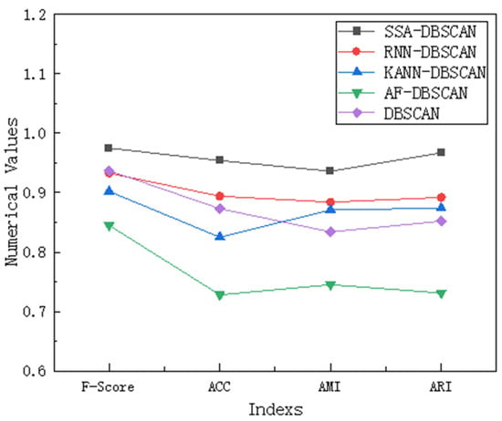
Figure 6.
Comparison of indicators for different algorithms.
6. Conclusions
Clustering is a commonly used technique in data mining to discover natural distributions and potential structures in data. The DBSCAN algorithm is a widely used density-based clustering algorithm that can automatically identify noise and perform clustering in arbitrary shapes. However, the clustering quality is significantly influenced by the parameters. To address this issue, this paper proposes an SSA-optimized DBSCAN algorithm, SSA-DBSCAN, which employs the silhouette coefficient as the fitness function to optimize the DBSCAN input parameters Eps and MinPts. This approach addresses the algorithm’s sensitivity to input parameters and allows DBSCAN to perform self-adaptive clustering. Performance tests on classic synthetic datasets, UCI real-world datasets, and image segmentation show that the clustering performance of SSA-DBSCAN outperforms that of the DBSCAN algorithm and its improved algorithms, such as KANN-DBSCAN, AF-DBSCAN, and other algorithms. Moreover, the proposed method has broad application prospects in fields such as remote sensing image analysis, medical image segmentation, video surveillance, environmental monitoring, and anomaly detection in high-dimensional data. However, the time complexity of SSA-DBSCAN remains similar to that of DBSCAN. Improving the running speed of algorithms requires additional research.
Author Contributions
Methodology, S.Z. (Shibo Zhou) and S.Z. (Shuntao Zhang); data curation, S.Z. (Shibo Zhou); resources, S.Z. (Shuntao Zhang); software, Z.H. and Z.L.; visualization, Z.L.; writing—original draft, Z.H.; and writing—review & editing, S.Z. (Shibo Zhou). All authors have read and agreed to the published version of the manuscript.
Funding
This research received no external funding.
Data Availability Statement
All research data used and provided in the paper are public. The needed sources are provided in the References.
Conflicts of Interest
The authors declare no conflicts of interest.
References
- Tan, S.K.; Wang, X. A novel two-stage omni-supervised face clustering algorithm. Pattern Anal. Appl. 2024, 27, 3. [Google Scholar] [CrossRef]
- Madrid-Herrera, L.; Chacon-Murguia, M.I.; Ramirez-Quintana, J.A. AENCIC: A method to estimate the number of clusters based on image complexity to be used in fuzzy clustering algorithms for image segmentation. Soft Comput. 2023, 28, 8561–8577. [Google Scholar] [CrossRef]
- Zhang, W. An improved DBSCAN algorithm for hazard recognition of obstacles in unmanned scenes. Soft Comput. 2023, 27, 18585–18604. [Google Scholar] [CrossRef]
- Kim, B.; Jang, H.J. Genetic-Based Keyword Matching DBSCAN in IoT for Discovering Adjacent Clusters. Comput. Model. Eng. Sci. 2023, 5, 20. [Google Scholar] [CrossRef]
- Ester, M. A Density-Based Algorithm for Discovering Clusters in Large Spatial Databases with Noise. Proc. Int. Conf. Knowl. Discov. Data Min. 1996, 96, 226–231. [Google Scholar]
- Lu, S.; Cheng, L.; Lu, Z.; Huang, Q.; Khan, B.A. A Self-Adaptive Grey DBSCAN Clustering Method. J. Grey Syst. 2022, 34, 4. [Google Scholar]
- Cao, P.; Yang, C.; Shi, L.; Wu, H. PSO-DBSCAN and SCGAN-Based Unknown Radar Signal Processing Method. Syst. Eng. Electron. 2022, 44, 4. [Google Scholar]
- Li, H.; Liu, X.; Li, T.; Gan, R. A novel density-based clustering algorithm using the nearest neighbor graph. Pattern Recognit. 2020, 102, 107206. [Google Scholar] [CrossRef]
- Wang, G.; Lin, G. Improved Adaptive Parameter DBSCAN Clustering Algorithm. Comput. Eng. Appl. 2020, 56, 45–51. [Google Scholar]
- Li, Y.; Wang, Y.; Song, H.X. GNN-DBSCAN: A new density-based algorithm using grid and the nearest neighbor. J. Intell. Fuzzy Syst. 2021, 41, 7589–7601. [Google Scholar]
- Sunita, J.; Parag, K. Algorithm to Determine ε-Distance Parameter in Density Based Clustering. Expert Syst. Appl. 2014, 41, 2939–2946. [Google Scholar]
- Bryant, A.C.; Cios, K.J. RNN-DBSCAN: A Density-Based Clustering Algorithm Using Reverse Nearest Neighbor Density Estimates. IEEE Trans. Knowl. Data Eng. 2018, 30, 1109–1121. [Google Scholar] [CrossRef]
- Li, W.; Yan, S.; Jiang, Y.; Zhang, S.; Wang, C. Research on the Method of Self-Adaptive Determination of DBSCAN Algorithm Parameters. Comput. Eng. Appl. 2019, 55, 1–7. [Google Scholar]
- Li, Y.; Yang, Z.; Jiao, S.; Li, Y. Partition KMNN-DBSCAN Algorithm and Its Application in Extraction of Rail Damage Data. Math. Probl. Eng. 2022, 2022, 4699573. [Google Scholar] [CrossRef]
- Zhou, Z.; Wang, J.; Zhu, S.; Sun, Z. An improved adaptive and fast AF-DBSCAN clustering algorithm. CAAI Trans. Intell. Syst. 2016, 11, 93–98. [Google Scholar]
- Chen, S.H.; Yi, M.L.; Zhang, Y.X. Wafer graph preprocessing based on optimized DBSCAN clustering algorithm. J. Control Decis. 2021, 36, 2713–2721. [Google Scholar]
- Juan, C.P.L.; Junlian, S.P. An unsupervised pattern recognition methodology based on factor analysis and a genetic-DBSCAN algorithm to infer operational conditions from strain measurements in structural applications. Chin. J. Aeronaut. 2021, 34, 165–181. [Google Scholar]
- Zhang, X.; Zhou, S. WOA-DBSCAN: Application of Whale Optimization Algorithm in DBSCAN Parameter Adaption. IEEE Access 2023, 11, 91861–91878. [Google Scholar] [CrossRef]
- Wang, Z.; Ye, Z.; Du, Y.; Mao, Y.; Liu, Y.; Wu, Z.; Wang, J. AMD-DBSCAN: An Adaptive Multi-density DBSCAN for datasets of extremely variable density. In Proceedings of the 9th IEEE International Conference on Data Science and Advanced Analytics (DSAA), Shenzhen, China, 13–16 October 2022; pp. 116–125. [Google Scholar] [CrossRef]
- Yang, Y.; Qian, C.; Li, H.; Gao, Y.; Wu, J.; Liu, C.J.; Zhao, S. An Efficient DBSCAN Optimized by Arithmetic Optimization Algorithm with Opposition-Based Learning. J. Supercomput. 2022, 78, 19566–19604. [Google Scholar] [CrossRef]
- Xue, J. Research and Application of a Novel Swarm Intelligence Optimization Technology. Master’s Thesis, Donghua University, Shanghai, China, 2020. [Google Scholar]
- Gao, S.; Zhou, X.; Li, S. Density Ratio-Based Density Peak Clustering Algorithm. Comput. Eng. Appl. 2017, 53, 8. [Google Scholar]
- Rodriguez, A.; Laio, A. Clustering by fast search and find of density peaks. Science 2014, 344, 1492. [Google Scholar] [CrossRef] [PubMed]
- Dong, X.; Cheng, C. Kernel Density Estimation-Based K-CFSFDP Clustering Algorithm. Comput. Sci. 2018, 45, 5. [Google Scholar]
- Wang, Y.; Zhang, G. Density Peak Clustering Algorithm for Automatically Determining Cluster Centers. Comput. Eng. Appl. 2018, 54, 6. [Google Scholar]
- Hartigan, J.A.; Wong, M.A. A K-Means clustering algorithm. JR Stat. Soc. Ser. C-Appl. Stat. 1979, 28, 100–108. [Google Scholar]
- Manaa, M.; Obaid, A.J.; Dosh, M. Unsupervised Approach for Email Spam Filtering using Data Mining. EAI Endorsed Trans. Energy Web 2018, 8, e3. [Google Scholar] [CrossRef]
- Huang, S.X.; Luo, J.W.; Pu, K.X.; Wu, M.; Chaudhary, G. Diagnosis system of microscopic hyperspectral image of hepatobiliary tumors based on convolutional neural network. Comput. Intel. Neurosc. 2022, 2022, 3794844. [Google Scholar] [CrossRef]
- Ping, X.; Yang, F.B.; Zhang, H.G.; Xing, C.D.; Zhang, W.J.; Wang, Y. Evaluation of hybrid forecasting methods for organic Rankine cycle: Unsupervised learning-based outlier removal and partial mutual information-based feature selection. Appl. Energ. 2022, 311, 118682. [Google Scholar] [CrossRef]
- Unnikrishnan, R.; Pantofaru, C.; Hebert, M. Toward Objective Evaluation of Image Segmentation Algorithms. IEEE Trans. Pattern Anal. Mach. Intell. 2007, 29, 929. [Google Scholar] [CrossRef]
- Wang, X.; Tang, Y.; Masnou, S.; Chen, L. A Global/Local Affinity Graph for Image Segmentation. Proc. ACM Conf. Comput. Sci. 1988, 24, 1399–1411. [Google Scholar]
Disclaimer/Publisher’s Note: The statements, opinions and data contained in all publications are solely those of the individual author(s) and contributor(s) and not of MDPI and/or the editor(s). MDPI and/or the editor(s) disclaim responsibility for any injury to people or property resulting from any ideas, methods, instructions or products referred to in the content. |
© 2025 by the authors. Licensee MDPI, Basel, Switzerland. This article is an open access article distributed under the terms and conditions of the Creative Commons Attribution (CC BY) license (https://creativecommons.org/licenses/by/4.0/).