Spiking Neural Networks Optimized by Improved Cuckoo Search Algorithm: A Model for Financial Time Series Forecasting

Abstract

Financial Time Series Forecasting (TSF) remains a critical challenge in Artificial Intelligence (AI) due to the inherent complexity of financial data, characterized by strong non-linearity, dynamic non-stationarity, and multi-factor coupling. To address the performance limitations of Spiking Neural Networks (SNNs) caused by hyperparameter sensitivity, this study proposes an SNN model optimized by an Improved Cuckoo Search (ICS) algorithm (termed ICS-SNN). The ICS algorithm enhances global search capability through piecewise-mapping-based population initialization and introduces a dynamic discovery probability mechanism that adaptively increases with iteration rounds, thereby balancing exploration and exploitation. Applied to futures market price difference prediction, experimental results demonstrate that ICS-SNN achieves reductions of 13.82% in MAE, 21.27% in MSE, and 15.21% in MAPE, while improving the coefficient of determination (R²) from 0.9790 to 0.9822, compared to the baseline SNN. Furthermore, ICS-SNN significantly outperforms mainstream models such as Long Short-Term Memory (LSTM) and Backpropagation (BP) networks, reducing prediction errors by 10.8% (MAE) and 34.9% (MSE), respectively, without compromising computational efficiency. This work highlights that ICS-SNN provides a biologically plausible and computationally efficient framework for complex financial TSF, bridging the gap between neuromorphic principles and real-world financial analytics. The proposed method not only reduces manual intervention in hyperparameter tuning but also offers a scalable solution for high-frequency trading and multi-modal data fusion in future research.

1. Introduction

AI has advanced rapidly in recent decades, driven by breakthroughs in computational power and algorithmic innovation. Initially, Artificial Neural Networks (ANNs) were limited to performing simple tasks. With advancements in computational power, ANNs have evolved to tackle increasingly complex tasks. TSF in the financial field is precisely such a challenging problem. Its data are not only vast in quantity but also diverse in variety. Data of this problem usually have strong periodic characteristics, which are well structured, unstable, and influenced by many factors. The futures market is one of the key parts in the financial field. In today’s largest futures trading market, the cumulative trading volume in the futures market reached 8.501 billion lots, with a cumulative turnover of USD 56.851 trillion, representing year-on-year growth of 25.60% and 6.28%, respectively [1]. Arbitrage is common for futures operation, which has smoother profits and lower risks. How to predict price differences is a critical issue in arbitrage.

Formally, forecasting has been divided into nowcasting, very short term, short term, long, very long term, and so on. Nowcasting is a time series analysis task aiming to forecast the current state of an observed phenomenon. A very short-term forecast is a prediction of a few minutes to a day. And short term refers to forecasting activities where the target is relatively close to the present time and has a relatively short duration, ranging from daily to several months. They rely on recent data and are greatly affected by short-term fluctuations. Long-term and very long-term forecasting, typically encompassing a timeframe exceeding two years, are often undertaken at the strategic level. They have a high degree of uncertainty, and the model relies on assumptions and scenario analysis.

The techniques and methods for TSF can be divided into statistical methods, physical methods, time series analysis methods, hybrid methods, and so on. Statistical methods are based on mathematical formulas and probability assumptions, utilizing historical data modeling of time series to capture trends, seasonality, and residual components. They are suitable for short-term data volumes that require fast modeling and high interpretability requirements. Yule (1927) constructed an Autoregressive (AR) model to predict the number of sunspots, which was an earlier TSF model in econometric analysis [2]. After that, scholars further proposed the Moving Average (MA) model to analyze time series data. Slightly different from the AR model, the MA model uses the lag term of the white noise sequence to predict the explained variables. AR and MA models are suitable for stationary time series data. However, it has been found that most financial time series data usually have non-stationary characteristics [3]. For this reason, Box and Jenkins further proposed an Autoregressive Integrated Moving Average (ARIMA) model to deal with non-stationary time series data. The ARIMA model is relatively simple and can effectively deal with non-stationary financial time series data, so it has become a commonly used econometric model in the field of financial time series data prediction.

Physical methods are based on domain knowledge (physical laws, chemical equations, etc.) to construct mechanistic models, emphasizing causal relationships rather than pure data-driven approaches. They are suitable for scenarios where prediction results must strictly comply with physical laws. For example, weather forecasting uses models based on atmospheric dynamics.

The time series analysis methods focus on the decomposition of the intrinsic structure of time series and pattern recognition, emphasizing data-driven feature extraction. It is necessary to have a deep understanding of the internal structure of the sequence, such as trends and cycles. Non-linear Autoregressive (NAR) and Non-linear Autoregressive with Exogenous inputs (NARX) models are prominent examples of time series forecasting techniques that leverage recurrent structures to capture temporal dependencies effectively. NARX models extend traditional autoregressive models by incorporating external input variables, making them especially powerful for complex financial time series forecasting tasks.

Hybrid methods in time series forecasting combine multiple forecasting techniques, often blending statistical, machine learning, and/or physical models, to improve predictive accuracy and robustness. The idea behind hybrid methods is to take advantage of the strengths of each individual technique, while compensating for their weaknesses. For example, Luo proposed a hybrid model that combines Ensemble Empirical Mode Decomposition (EEMD), ARIMA, and Taylor expansion using a tracking differentiator to forecast financial time series [4].

Machine learning explores how to improve the performance of the model itself by means of computing and, using learning experience, it tries to find the relationships between the input data. Yu Z et al.’s Local Linear Embedding Dimensionality Reduction (LLE) algorithm is chosen to reduce the dimensionality of the factors affecting the stock price and the dimensionality-reduced data are used as a new input variable to the BP neural network for stock price prediction [5]. Another commonly used machine learning algorithm is Support Vector Machine (SVM). SVM avoids the problem of overfitting and improves the prediction ability of out-of-sample data. Stock market data have the characteristics of high noise and complex dimensions, while artificial neural networks often show inconsistency in the prediction of noise data. SVM is more suitable for financial time series data prediction [6]. Kuran introduced the use of SVM and ANN as prediction algorithms and raised challenges such as time constraints, current scenarios, data limitations, and cold start issues [7]. Random Forest (RF) is an ensemble learning method primarily used for classification and regression tasks. Although it was not originally designed for time series prediction, with appropriate adjustments and feature engineering, random forests can also be effectively applied to time series prediction problems. Fan proposed a hybrid model that combines the Random Forest (RF) model with the mean generation function model, which outperforms the original model based on selected prediction accuracy indicators in terms of peak–valley performance in highly volatile data [8].

Transformer-based models have shown excellent performance in the TSF field, and the latest Mamba has been proven to outperform Transformer in many aspects, not only with strong performance but also by reducing memory and computational overhead. Large Language Models (LLMs) have been applied in many fields and have developed rapidly in recent years. Wang’s experiment showed that Mamba exhibits remarkable potential to outperform Transformer in TSF tasks [9]. As a classic machine learning task, TSF has recently been boosted by LLMs. Tang‘s study shows that LLMs perform well in predicting time series with clear patterns and trends but face challenges in the absence of periodic datasets. He also proves Mamba shows great potential to surpass Transformer in TSF tasks [10]. Multi-variate time series prediction is a persistent challenge in various disciplines. On this issue, Cai proposed MSGNet, an advanced deep learning model aimed at using frequency domain analysis and adaptive graph convolution to capture intersequence correlations that vary across multiple time scales [11].

An ANN is a representative method that is applicable to all short-term, recent, and long-term data. The very first generation of ANNs had single-layer computational neurons, which made them capable of handling some linearly separable problems. The second generation of ANNs used multiple hidden layers to replace the original single feature layer in the perception and used the Backpropagation (BP) algorithm to calculate network parameters. But an increasing number of hidden layers and neurons require more computing resources. Meanwhile, the explainability becomes more difficult to ensure. Known as third-generation ANNs, SNNs can be more energy efficient than traditional artificial neural networks because they use spike-based signaling, which requires less energy to transmit than continuous signals. SNNs can also use the timing of spikes to process temporal information, such as sequences of events, so they have a greater advantage in TSF problems theoretically.

Shallow-level machine learning algorithms such as SVM and BP neural networks have great limitations in dealing with complex and high-dimensional data, and there are many problems, such as the disaster of dimensionality and inefficient feature representation [12]. Deep learning is a representation learning method with multi-level representation, which is obtained by superimposing multi-layer simple but non-linear modules. Each module converts the representation of each layer (starting from the input layer) into a more abstract representation of the next layer. As long as there are enough of these transformations, it can learn very complex functions [13]. Tsantekidis et al. applied a Convolutional Neural Network (CNN) to stock price prediction [14]. The results show that the prediction effect of this method is better than that of BP and SVM. Hsieh et al. pointed out that the structure of a Recurrent Neural Network (RNN) is simpler than that of a traditional artificial neural network [15], and it is more suitable for financial TSF prediction. An LSTM neural network is a form of RNN which can effectively deal with the problem of long-term dependence of sequences. Fischer and Krauss’s experiment showed that LSTM neural networks can extract important information from financial TSF data with a lot of noise [16].

Compared with previous generations of ANNs, SNNs have been the subject of much less research on TSF problems. The training and debugging process of SNNs is relatively complex. Training SNNs is inherently more complex than for traditional neural networks due to their reliance on temporal dynamics and signal accumulation mechanisms. In addition, due to the high biological rationality of SNNs and their relatively complex mathematical models, the debugging process may also be more difficult. Despite the difficulty, there has been progress. Matenczuk compared the performance of traditional neural networks and SNNs for financial TSF [17]. He found that there is a lack of information about encoding methods, learning methods, network structures, and neural models for SNNs, which hinders comparison, reproducibility, and replication. Reid D used SNNs in financial time series prediction, and he applied a Polychronous Spiking Network (PSN) to exploit the temporal characteristics of the spiking neural model in an appropriate way [18]. Abou Hassan proposed predictive and explainable modeling of stock price time series, integrated with online news, as a method, based on SNNs, for an integrated predictive modeling of multi-modal time series [19].

However, the SNN is still a relatively new and developing field, with some limitations in its use. From the traditional neural networks, through deep neural networks, to the recently emerging LSTM, they all do a good job in stock price forecasting. The SNN is rarely used in predictions compared to the previous generation. One reason is that there are so many hyperparameters in SNNs, so it is too hard to optimize them for making the best network to fit the specific problems. In most cases, these hyperparameters are manually adjusted by researchers, but this method has obvious drawbacks:

• Time is often wasted in the intervals between each experiment run. If a trial run ends, researchers cannot guarantee a timely start of the next one.
• Each experiment requires a considerable amount of effort, and researchers need to analyze the results and determine the direction of the next parameter adjustment.
• Researchers usually tend to choose aesthetically pleasing numbers as parameters, such as 200, 1150, or 0.55. This approach increases the likelihood of missing the optimal numbers, even though they may not look as appealing.

Therefore, biomimetic algorithms are good choices to find better hyperparameters, which can be inspired by the corresponding characteristics of biological systems, providing new design ideas and principles for engineering technology. The CS algorithm is a typical representation of them. But the combination of the original CS and SNNs is not satisfactory enough. Therefore, we proposed the ICS algorithm.

The work described in this article about ICS-SNN is summarized as follows:

• Change the initialization method of the cuckoo search algorithm and replace the discovery probability with a fixed value with a variable that increases with the number of iterations;
• Choose the proper hyperparameters for the SNN model and use the ICS to optimize them;
• Compare the performance of ICS-SNN, CS-SNN, and other models by using futures market data.

To illustrate the above work, the structure of the article has been arranged as follows: Section 2 is divided into three parts, elaborating on SNN, ICS, and how to combine the two in detail, respectively; Section 3 contains the data processing, test function, the metrics we used, and the results of our experiments; Section 4 is the discussion; and Section 5 is the conclusions.

2. Materials and Methods

2.1. SNN

Unlike most neural networks we know, SNNs use spikes to encode data [20,21]. As the third generation of ANNs, the SNN draws more help from the human brain, so it can act more like brain nerve cells: its neurons spike only when they receive important information or the environment around them undergoes tremendous changes. Under this understanding, SNNs are inherently suited to managing highly non-linear and temporally based input data that traditional neural networks struggle with [18].

The neurons of SNNs are created by imitating biological neural cells, which are mainly composed of dendrites, cell bodies, and axons. The function of dendrites is to collect signals inputted by other elements and transmit them to the cell body. When the accumulation of current received by the cell body causes a change in the membrane potential of the neuron to exceed a certain threshold, a nerve pulse will be generated. Pulses can travel along the axon and then through the synapses at the end of the axon. This completes the process by which presynaptic neurons transmit signals to postsynaptic neurons. With regard to the dynamic characteristics of neuron membrane potential and the process of pulse emission, researchers have established a variety of theoretical models of pulse neurons. Because the pulse neuron is the basic unit of the SNN, it is necessary to understand the neuron model we use in this paper before describing the research of pulse neural networks.

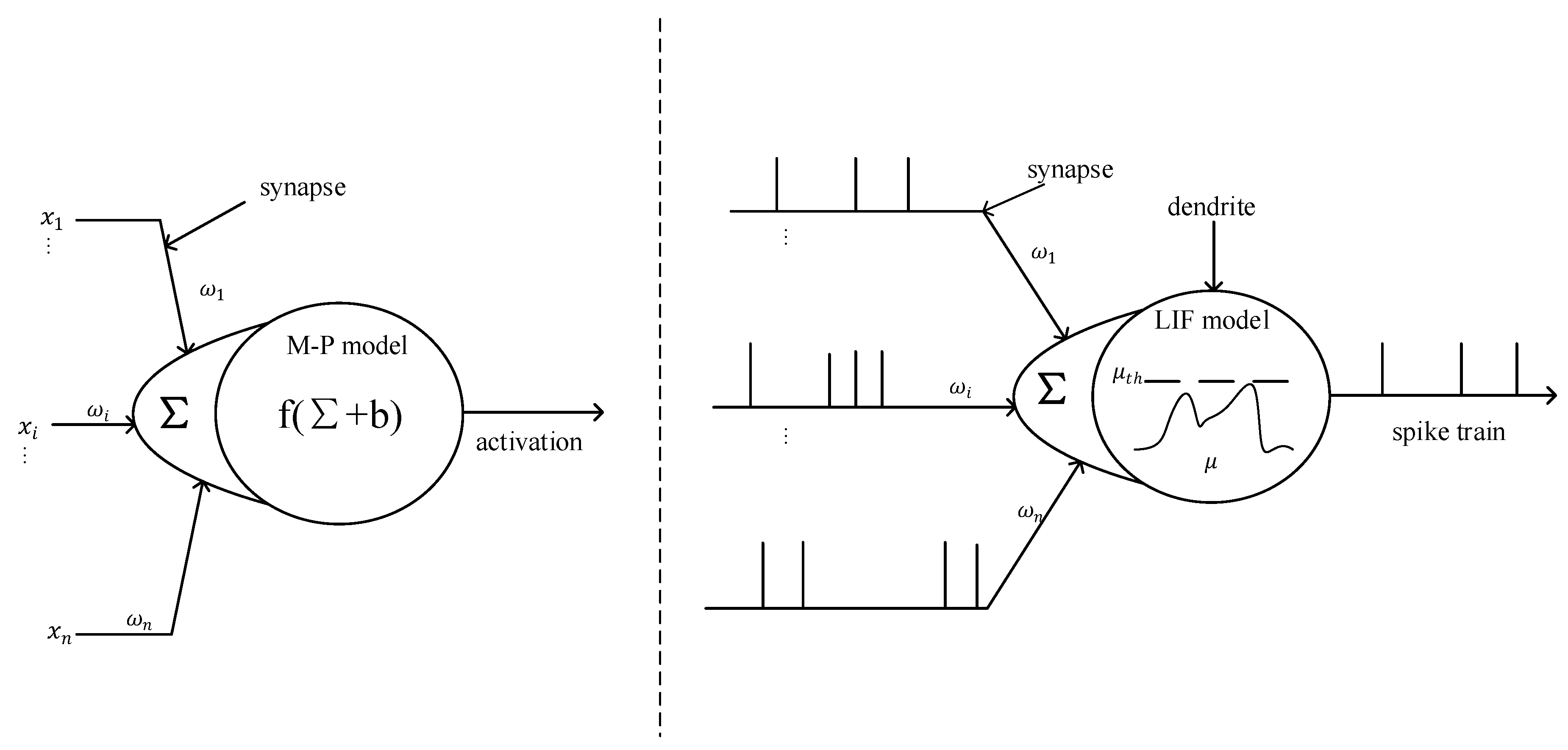
Most current neural networks are based on the McCulloch–Pitts (M-P) model. Its basic theory is to formalize neurons into an activation function composite with the form of a weighted sum, as shown in the left half of Figure 1. Although the M-P model is widely used in the field of deep learning, it is still far from the cell structure of real neurons. In comparison, SNNs use biologically closer spiking neurons as basic computing units to process information non-linearly. Different types of spiking neuron models describe the changes in cell membrane potential and the mechanism of pulse generation at different levels of detail [22].

The M-P model can be explained as follows:

$$y=f(\sum _{i=1}^n{w}_i{x}_i+b)$$

(1)

where $w_i$ represents the weight corresponding to the $i$-th input signal $x_i$. $b$ is a bias term used to adjust the activation threshold of neurons. And $f(\ast )$ is the activation function.

In this study, we used Leaky Integrate and Fire (LIF) as the computing unit. The schematic diagram of its structure is shown in the right half of Figure 1. The biggest difference between M-P and LIF models is the information processing mechanism. The M-P model is based on real value calculation, while LIF processes information based on spiking sequences with time information.

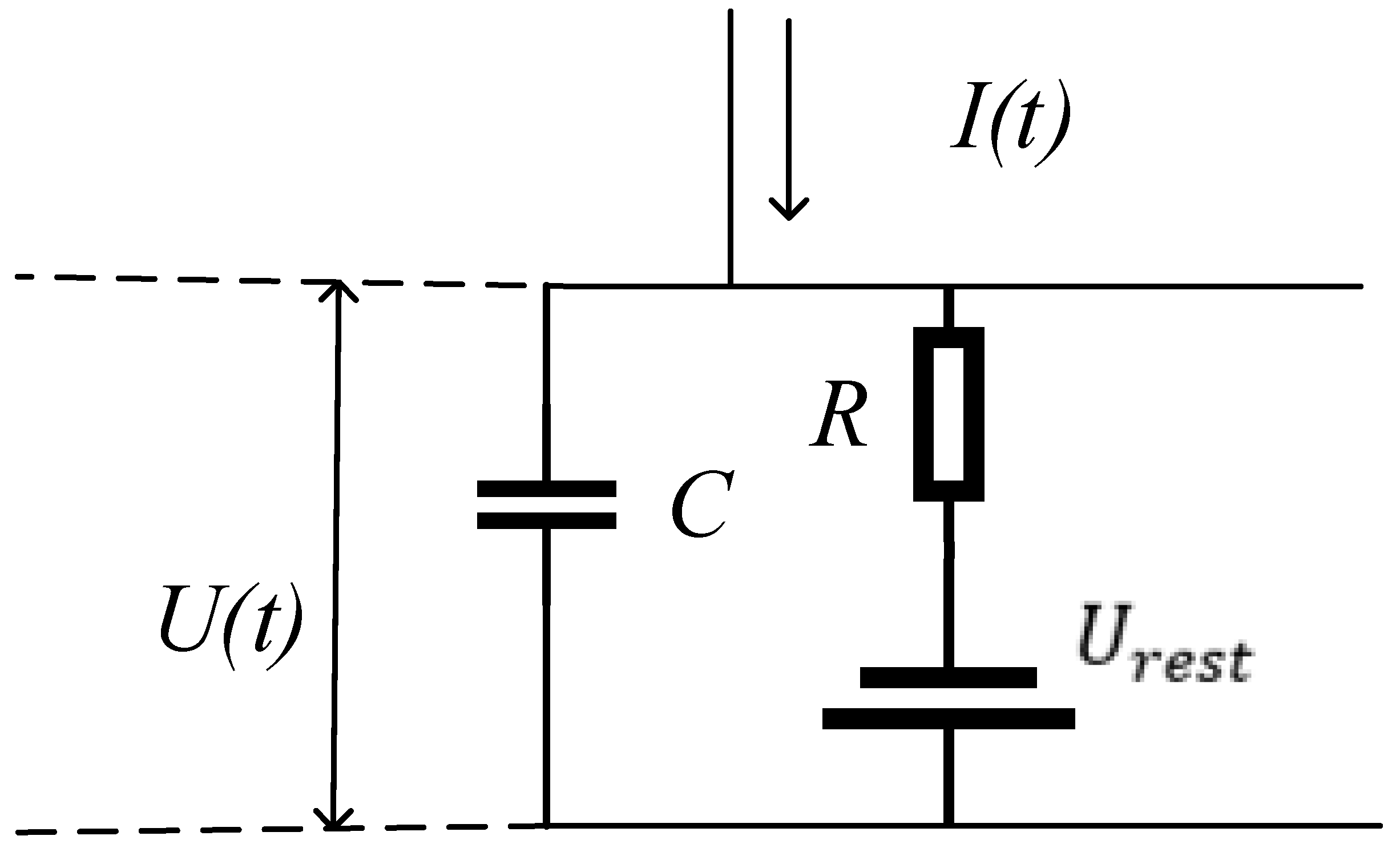
The LIF model is simple but effective when SNNs are used in financial prediction. The integrated firing model (Integrate and Fire, I&F) was proposed by Lapicque et al. in 1907 [23]. Due to the limitations of the conditions at that time, the mechanism of action potential is not clear, so the process of action potential is simplified as follows: when the membrane potential reaches the threshold, the neuron will excite the pulse, and the membrane potential falls back to the resting value, so the I&F neurons do not conform to the biological principle. Theoretically, the dynamic performance of biological neuron membrane potential should have three key characteristics: leakage, accumulation, and threshold excitation. The LIF neuron model is developed on the basis of the I&F model, which not only retains the above three characteristics but also simplifies the generation process of the action potential, which reduces the computational complexity and has better biological interpretability. The LIF model can be explained as follows:

$$\tau {\displaystyle \frac{dU}{dt}}=-\left(U-U_{rest}\right)+R\times I_{in}(t)$$

(2)

$$if U>U_{th}, U\leftarrow U_{reset}$$

(3)

where $\tau$ expresses the membrane time constant of the cell. As the firing time of a neuronal pulse is 1 ms generally, $\tau$ takes a value of 10 ms in most cases, which is larger than the duration of pulse emission. $U_{rest}$ is a constant parameter, which means the resting potential of the fine cell membrane. $I_{in}\left(t\right)$ is the value of input current, and $R$ is the cell membrane impedance. Equation (3) means, once the membrane potential $U$ exceeds the threshold $U_{th}$, it is considered that the neuron has issued a pulse; $U_{reset}$ represents the reset membrane potential value after the neuron generates a pulse.

The equivalent circuit diagram of the LIF model is shown in Figure 2.

While TSF’s data consist of a large number of time steps, LIF cannot maintain information from history data for a long time. To solve this problem, Recurrent LIF (RLIF) adds a feedback loop based on LIF. RLIF builds on the standard RNN, which enables the network to use relationships along several time steps for the prediction of the current time step [24]. Compared to non-recursive loops, the RNN can retain information for a relatively long time step [25]. The activation function of the LIF model in Figure 1 can be formulated as

$${\varphi }_{spk,t}^{\left(l\right)}=\left\{\begin{array}{c}1, U_{\eta ,t}^{\left(l\right)}\ge U_{thr,\eta }^{\left(l\right)} \\ 0, U_{\eta ,t}^{\left(l\right)}<U_{thr,\eta }^{\left(l\right)}\end{array}\right.$$

(4)

RLIF formulation can be described as follows:

$$U_{\eta ,t}^{\left(l\right)}={\beta }_{\eta }^{\left(l\right)}{U}_{\eta ,t-1}^{\left(l\right)}+W_{\eta }^{\left(l\right)}{h}_t^{(l-1)}+V_{\eta }^{\left(l\right)}{h}_{t-1}^{(l-1)}-{\varphi }_{spk,t-1}^{\left(l\right)}{U}_{thr,\eta }^{\left(l\right)}$$

(5)

where $U_{\eta ,t}^{\left(l\right)}$ is the membrane potential of the η-th neural unit at time t, $U_{thr,\eta }^{\left(l\right)}$ denotes the membrane threshold, ${\beta }_{\eta }^{\left(l\right)}$ is the membrane potential decay rate, and $W_{\eta }^{\left(l\right)}{h}_t^{(l-1)}$ is the standard ANN weight multiplied with the preceding layer at the current time step. And $V_{\eta }^{\left(l\right)}$ is the additional recurrent weights.

Finally, it can be used to train the following parameters:

$${\theta }_{RLIF}=\left\{W_{\eta }^{\left(l\right)},V_{\eta }^{\left(l\right)},{\beta }_{\eta }^{\left(l\right)},U_{thr,\eta }^{\left(l\right)}\right\}$$

(6)

2.2. ICS

The Cuckoo Search (CS) algorithm is inspired by the brood parasitism of cuckoo birds, a strategy that enhances offspring survival through nest parasitism [26]. The algorithm is inspired by the specific parasitic feeding behavior of cuckoo bird species, where certain species lay eggs in other birds’ nests and may remove other birds’ eggs to increase the hatching probability of their own eggs. There are three basic types of brood parasitism:

• Some host birds directly conflict with invading cuckoo birds. The host bird has a probability of discovering that the egg is not its own, then the host bird will discard eggs that are not its own or abandon its original nest to build a new one;
• Some species mimic the color of host eggs to reduce the likelihood of eggs being abandoned and improve reproductive ability;
• Some species usually choose a nest where the host bird has just laid eggs. The cuckoo bird’s eggs hatch earlier than the host’s eggs. Once the first cuckoo bird chick hatches, it instinctively and blindly pushes out the host bird’s eggs, increasing the share of food provided by the host.

The conversion relationship between the egg’s position and time is as follows:

$$X_{t+1}=X_t+\alpha ⨂Levy\left(\beta \right)$$

(7)

where $X_t$ is the position at time t, $X_{t+1}$ is the next position after time $t$. And α is the step size scaling factor, and in most questions we can set $\alpha$ as 1, ⨂ is the dot product operator, and Lévy(β) represents the Lévy flight.

Lévy flight is a random walking process, in which the length and direction of the step are determined by the Lévy distribution. The Lévy distribution is a probability distribution with long-tailed distribution characteristics. In the cuckoo algorithm, the Lévy flight strategy is used to update the position of cuckoo individuals in order to search for better solutions.

The step size of Lévy flight is a random walk that follows a heavy-tailed distribution. After multiple walks, the flight step size starting from the original point usually tends to stabilize. The Lévy distribution, named by mathematician Paul Lévy, is a continuous probability distribution. The specific formula is shown in Equation (8).

$$Levy\left(\beta \right)={\displaystyle \frac{u}{{\left|v\right|}^{1/\beta }}}$$

(8)

In Equation (8), $\beta$ usually takes a value between [0, 2], with a value of 1.8 here, then $u$ and $v$ should follow a normal distribution with zero mean and variances defined in Equations (9) and (10).

$${\sigma }_u={\left\{{\displaystyle \frac{\mathsf{\Gamma }(1+\beta )\sin (\beta \pi /2)}{\mathsf{\Gamma }\left(\right(1+\beta )/2)2^{(\beta -1)/2}\beta }}\right\}}^{1/\beta }$$

(9)

$${\sigma }_v=1$$

(10)

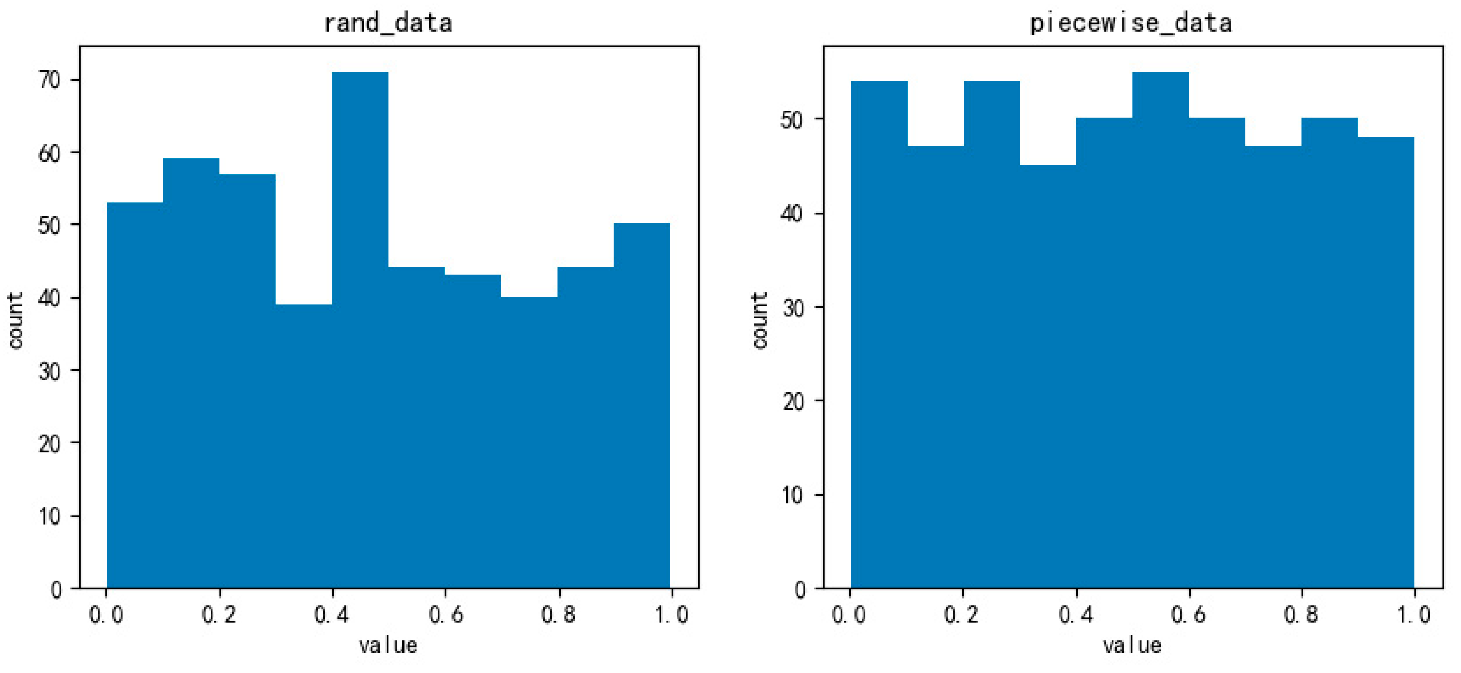
Before the very first search, we need to obtain a position to start. The original cuckoo algorithm initializes the position with a random solution, which is too stochastic to obtain uniformly distributed positions. Therefore, we choose piecewise mapping to obtain a more uniform distribution. The piecewise mapping is as follows:

$$f\left(x\right)=\left\{\begin{array}{c}{\displaystyle \frac{x\left(t\right)}{p}}, 0\le x\left(t\right)<p\\ {\displaystyle \frac{x\left(t\right)-p}{0.5-p}}, p\le x\left(t\right)<0.5\\ {\displaystyle \frac{1-p-x\left(t\right)}{0.5-p}}, 0.5\le x\left(t\right)<1-p\\ {\displaystyle \frac{1-x\left(t\right)}{p}}, 1-p\le x\left(t\right)<1\end{array} \right.$$

(11)

In Equation (11), $p$ is 0~0.5 and $x\left(1\right)$ is a random value. We used 500 random values and cycled the piecewise method the same number of times. The scatter and distribution histograms are shown in Figure 3.

The probability that the host bird discovers the egg is usually a fixed value. It is convenient for calculation but surely does not conform to natural conventions. The probability is modified to calculate through a formula as follows:

$$p=p_{min}+{(p}_{max}-p_{min})\times e^{i_n-i_t}$$

(12)

where $p$ is the final probability, $p_{min}$ is the minimum probability, $p_{max}$ is the maximum probability, $i_n$ is the current iteration round, and $i_t$ is the total iteration rounds. The probability increases with the number of iteration rounds, which is more in line with reality.

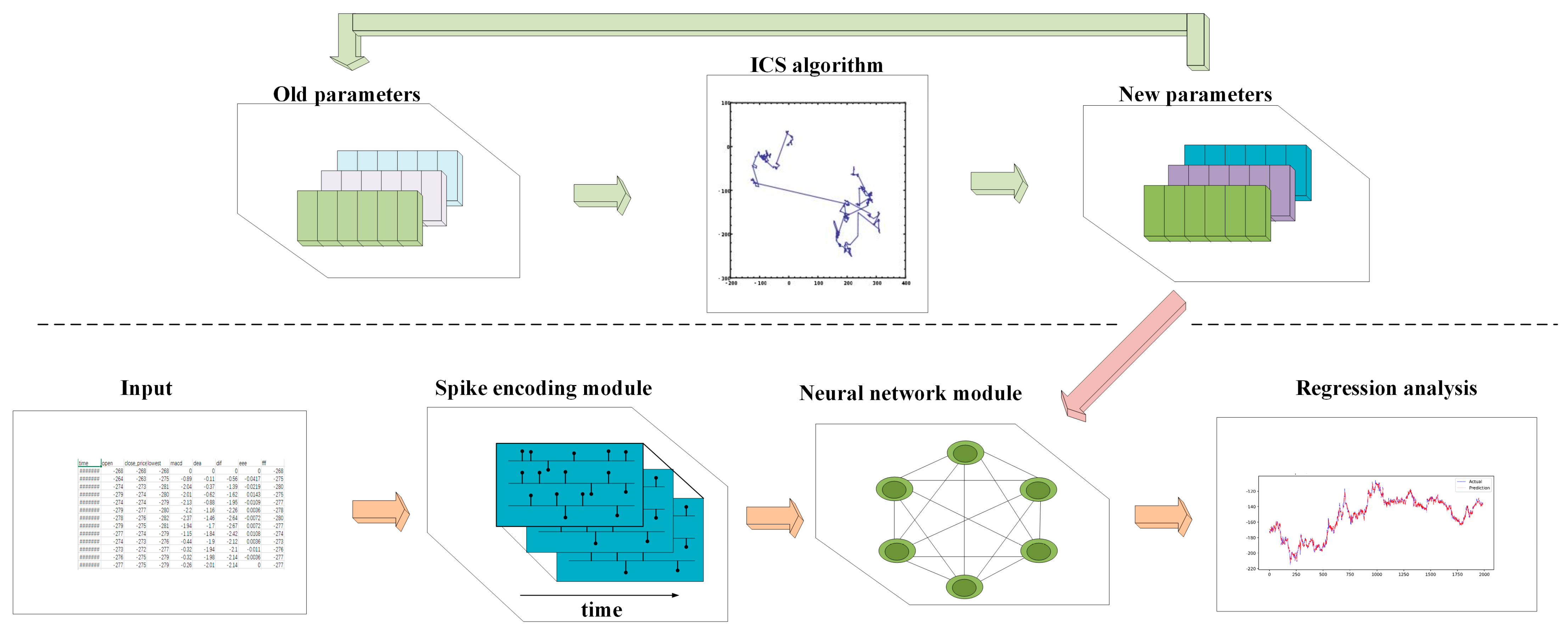
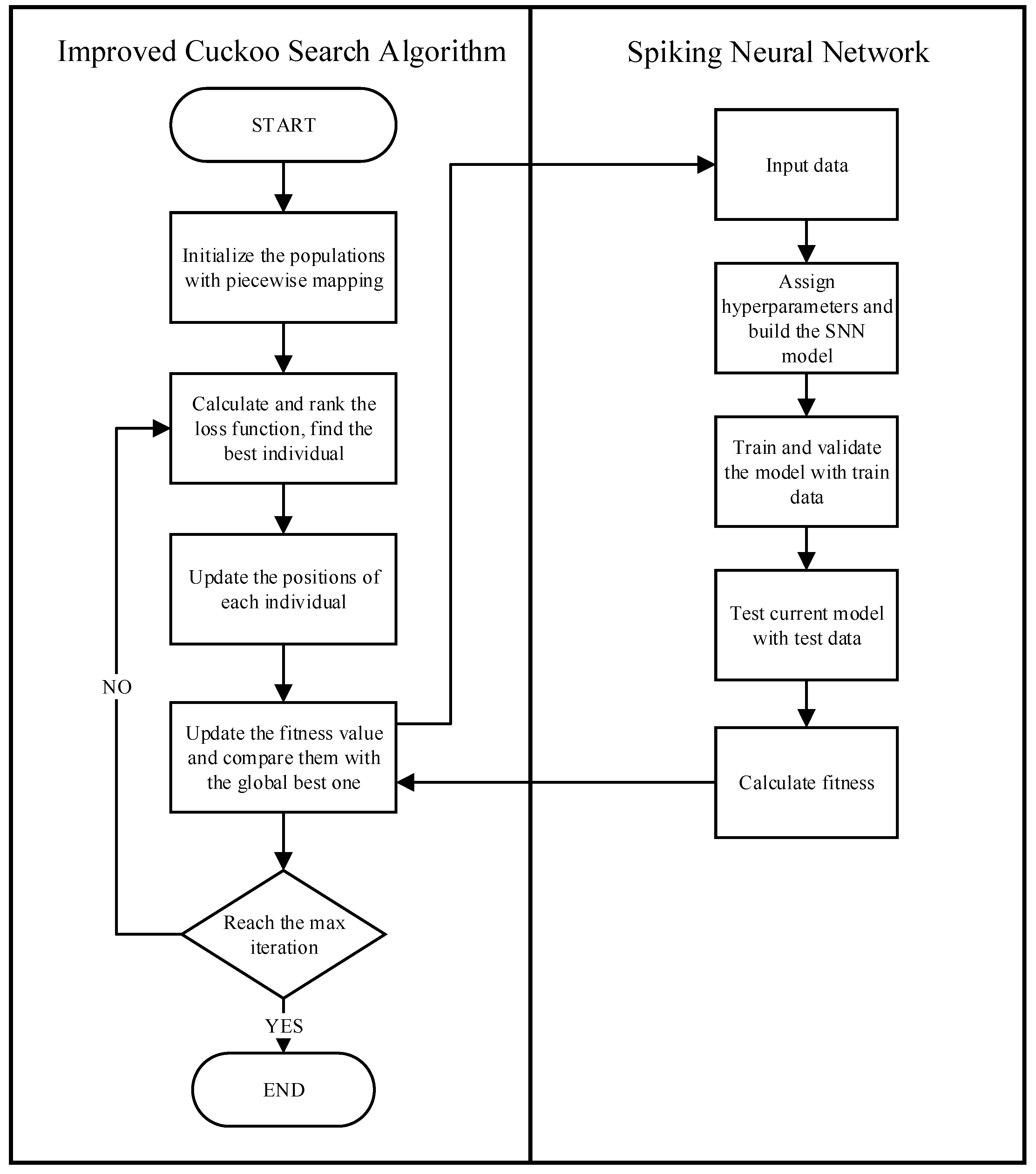
2.3. ICS-SNN

As shown in Figure 4, ICS-SNN is the new model that combines the previous two methods together. ICS is responsible for continuously selecting new hyperparameters, and the SNN needs to incorporate these parameters into the model, then train and validate their effectiveness. There are several hyperparameters which used to be changed manually when SNNs are used as shown in

Table 1. Selected hyperparameters and their Ranges.

Hyperparameter Name	Search Range
Time step	[5, 20]
Neuron number	[500, 2000]
Batch size	[10,000, 20,000]
Scaler scope	[4, 6]
Decay rate	[0.5, 0.8]

.

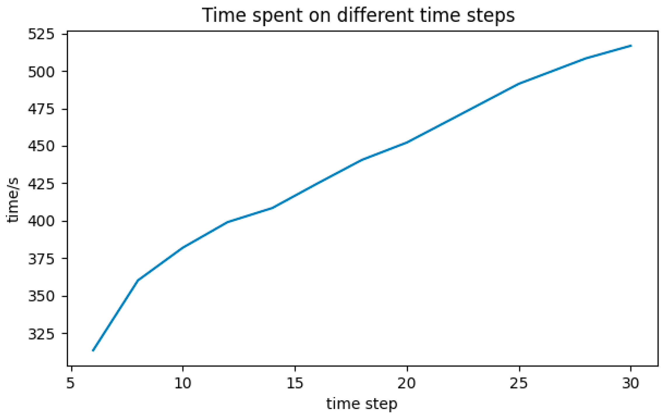
Time step. Time step means how many data are used to predict the price for the next time. If the number is set to be small, it is very likely that the model does not have enough prior knowledge to output the accurate value we expect. In contrast, if it is set to be too big, not only does it require more computing resources but it also takes more time to perform matrix operations. Time spent on different time steps is shown in Figure 5.

Count of Neurons. How to find the correct count of neurons for hidden layers is always a headache problem. A small quantity may result in underfitting, as the network may not learn correctly. However, excessive quantity may lead to overfitting, as learning too much from the network makes it impossible to generalize. Therefore, there must be an appropriate number of neurons to ensure good training.

Scaler Scope. After data normalization, the process of seeking the optimal solution becomes smoother and can converge to the optimal solution more quickly. “MinMaxScaler” is a method of data normalization used to scale data to a specified range. It maps the data to a specified minimum and maximum value by performing a linear transformation on the data.

$$X_{scaled}={\displaystyle \frac{\left(X-X_{min}\right)\times (B-A)}{X_{max}-X_{min}}}+A$$

(13)

where $X$ is one of the values which needs to be normalized, $X_{min}$ and $X_{max}$ are the minimum and maximum values of $X$. $A$ and $B$ are the specified minimum and maximum value we want $X$ to be limited to. Finally, $X_{scaled}$ is the value input in the model.

Batch Size. A small batch size increases computational time and causes severe gradient oscillations, hindering convergence. Conversely, an excessively large batch size reduces gradient diversity across batches, leading to local minima entrapment. The longer it takes to complete each epoch and the smoother the gradient between each iteration, the greater the batch size, which directly affects the mean and variance calculated by batch normalization, making them closer to the true mean and variance of the training set data distribution, thereby improving the regularization effect. Therefore, when computing resources allow, increasing batch size can not only accelerate training speed but also improve accuracy.

Membrane Potential Decay Rate. In the absence of input pulses, the membrane voltage decays over time due to the membrane decay rate.

Threshold. When the membrane potential exceeds the threshold of a neuron, the neuron will generate a pulse. The setting of the threshold is the triggering condition for pulse neurons to generate pulses and, usually, the threshold is a fixed parameter. Choosing an appropriate threshold has a significant impact on the pulse firing of neurons. Too high or too low a threshold may cause neurons to be unable to emit pulses correctly or frequently. And we consider the threshold as a hyperparameter in an attempt to bring great possibilities.

In the past, researchers always relied on experience to change parameters, which resulted in low accuracy, low efficiency, and time-consuming results. The ICS algorithm provides a way for automatically searching for solutions. So, it is natural to combine the ICS and SNNs, and we call it ICS-SNN. The flowchart of ICS-SNN is shown in Figure 6. The max iteration in the figure is not just a fixed value. During each iteration, if the quality of the current solution does not significantly improve, the search process is terminated as a convergence criterion.

2.4. Data Processing

The data used in this study are from Shanghai Futures Exchange. We obtained the original tick file from the Comprehensive Transaction Platform (CTP), then fixed the data as one-minute k-line files.

Due to the rare quotations on the market of unpopular products, the products we chose were Rebar (RB) and Hot Rolled Coil Plate (HC). RB and HC are almost the most popular products in the futures market, and this provides us with sufficient data. Furthermore, RB and HC are both products of black steel, so their price trends are highly fitting, and there is a strong correlation between them, which gives investors abundant arbitrage opportunities. We collected the tick data of RB and HC from 15 July 2020 to 23 March 2023 crossed over 654 days, and transformed the tick data to 1-min Kline data. Then, we subtracted RB’s closing price from HC’s closing price and finally obtained the price difference data.

3. Results

3.1. ADF Test

Before doing the experiment, we need to ensure that is there a cointegration relationship between the two. Firstly, we used the Augmented Dickey–Fuller (ADF) test to see if the two sequences are integrated of order one. The result is shown in

Table 2. ADF test.

Variety	ADF	p-Value	1%
RB	−73.51142	0.0	−3.43037912096488
HC	−62.22528	0.0	−3.430379122521149

.

From the results in

Table 3. Cointegration relationship test.

t-Statistic	p-Value	1%	5%	10%
−6.6336619	6.20974984 × 10−8	−3.89648876	−3.3361572	−3.04446888

, it can be seen that both sequences are integrated of order one. Then, we determine if there is a cointegration relationship between the two sequences.

From the results shown in

Table 4. Description of functions in CEC2019.

No	Description	Dimension	Range	F_min
F1	Storn’s Chebyshev Polynomial Fitting Problem	9	[8192, 8192]	1
F2	Inverse Hilbert Matrix Problem	16	[16,384, 16,384]	1
F3	Lennard-Jones minimum Energy Cluster	18	[4, 4]	1
F4	Rastrigin’s Function	10	[−100, 100]	1
F5	Griewangk’s Function	10	[−100, 100]	1
F6	Weierstrass Function	10	[−100, 100]	1
F7	Modified Schwefel’s Function	10	[−100, 100]	1
F8	Expanded Schaffer’s Function	10	[−100, 100]	1
F9	Happy Function	10	[−100, 100]	1
F10	Ackley Function	10	[−100, 100]	1

, it can be seen that the t-statistic value is less than 1% confidence, so there is a 99% confidence in rejecting the original hypothesis, and the p-value is also relatively small, so there is a cointegration relationship between RB and HC.

3.2. Test Function

To test the universality of ICS, we conducted CEC2019 on ICS. The CEC2019 function set is a highly effective benchmark function for testing the performance of metaheuristic algorithms. In CEC2019, the F1–F3 function has different dimensional values and ranges, while the F4–F10 function is a 10-dimension minimization problem. Due to the fact that many of the CEC2019 test functions are multi-modal, they are very challenging. CEC2019 problems are shown in

Table 5. Model parameters and package version and computer hardware.

Name	Value
GPU	RTX4060Ti
CPU	Intel Core i5 13600KF
CUDA	12.5
CuDNN	11.2
SnnTorch	0.8.1
Datasize	10,000
Train ratio	0.8

.

As shown in Figure 7, ICS performed better than CS in almost every function in CEC2019. The test results not only prove the generality, effectiveness, and performance advantages of the newly proposed ICS algorithm but they also demonstrate its potential and value in dealing with complex problems.

3.3. Metrics

To quantify the difference between predicted results and actual values, we need to choose proper loss functions. An excellent loss function not only needs to help researchers clearly understand the performance of the model but also needs to help to improve the model parameters. In machine learning, we want the predicted values to be infinitely close to the true values, so we need to minimize the difference. The choice of loss function is crucial in this process. In specific projects, some loss functions calculate a difference gradient that decreases quickly, while others decrease slowly.

In this study, we use the following metrics to evaluate the performance of the model: Mean Absolute Error (MAE), Mean Squared Error (MSE), Mean Absolute Percentage Error (MAPE), and Coefficient of Determination (R²). Their formulas are as follows:

$$MAE={\displaystyle \frac{1}{n}}\sum _{i=1}^n\left|{\widehat{y}}_i-y_i\right|$$

(14)

$$MSE={\displaystyle \frac{1}{n}}\sum _{i=1}^n{\left({\widehat{y}}_i-y_i\right)}^2$$

(15)

$$MAPE={\displaystyle \frac{100\%}{n}}\sum _{i=1}^n\left|{\displaystyle \frac{{\widehat{y}}_i-y_i}{y_i}}\right|$$

(16)

$$R^2=1-{\displaystyle \frac{{\sum }_i{\left({\widehat{y}}_i-y_i\right)}^2}{{\sum }_i{\left({\overline{y}}_i-y_i\right)}^2}}$$

(17)

where ${\widehat{y}}_i$ means the predicted value, $y_i$ means the true value, and $n$ is the number of samples. The smaller the values of MSE, MSE, and MAPE, the better our model performance. As for theR², the closer the value is to 1, the better performance will be. MAE is used to measure absolute error, MSE is more sensitive to large errors, MAPE facilitates understanding the relative error size, and R² reflects the model’s ability to explain variability.

3.4. Comparison Experiment

The specific Python version used in this study is 3.9.18, and the versions of other software and hardware are shown in

Table 6. Evaluation results of each model.

Model Name	MAE	MSE	MAPE	R2
ICS-SNN	2.3571	10.4675	0.0156	0.9822
CS-SNN	2.4709	11.2242	0.0163	0.9812
SNN	2.7351	13.2958	0.0184	0.9790
LSTM	2.6428	13.2309	0.0173	0.9779
BP	2.8884	16.0640	0.0192	0.9731
MLP	3.0191	16.9058	0.0202	0.9717

. Given the dataset size exceeding 180,000 samples, processing all data would impose prohibitive computational time and memory demands. Therefore, a subset of the data was selected for experimentation.

To demonstrate the improved model’s performance more intuitively, we conduct several different usual methods at the same time: LSTM, BP, and Multi-layer Perceptron (MLP). The results of metrics are shown in Figure 8.

4. Discussion

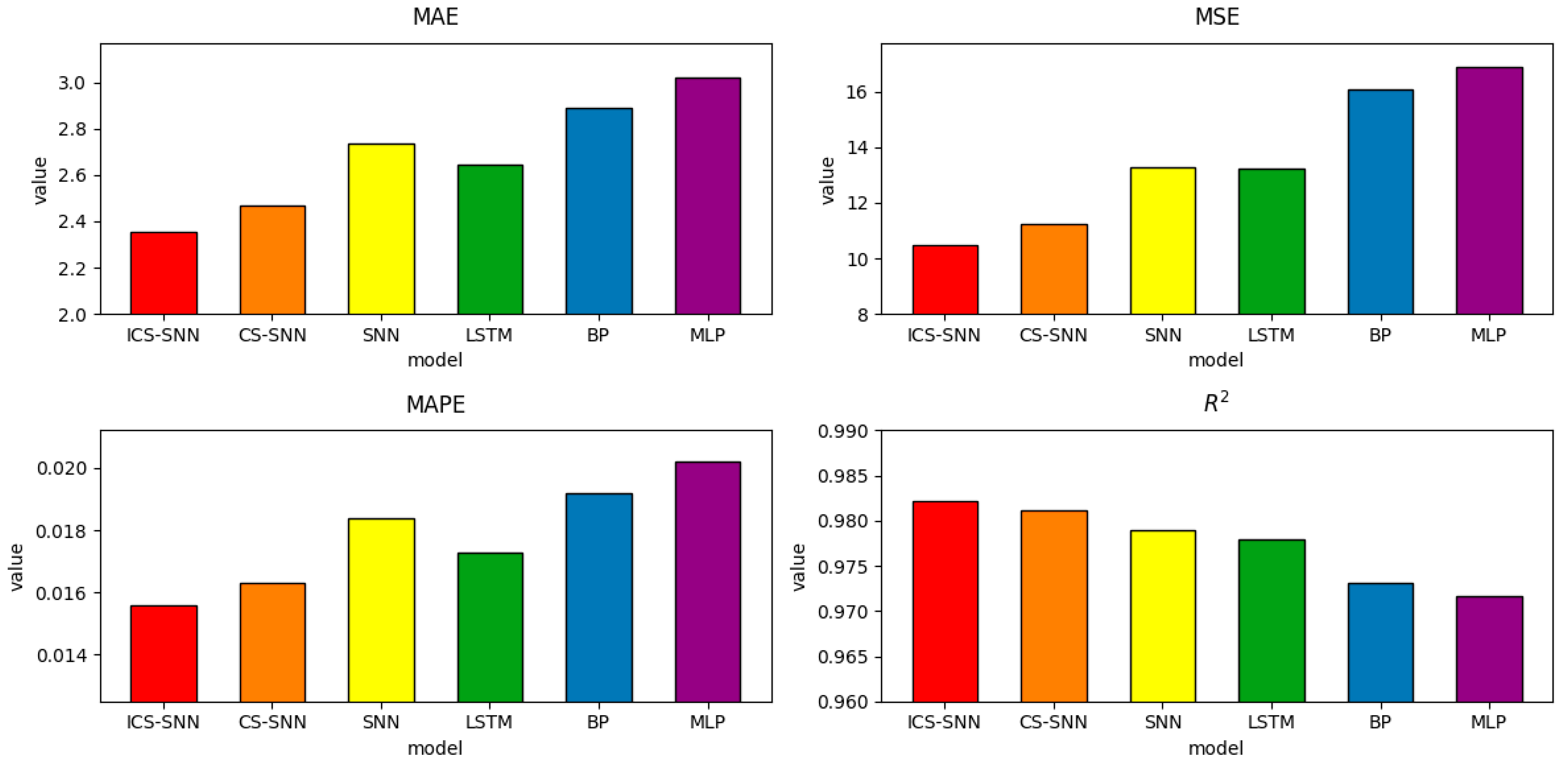
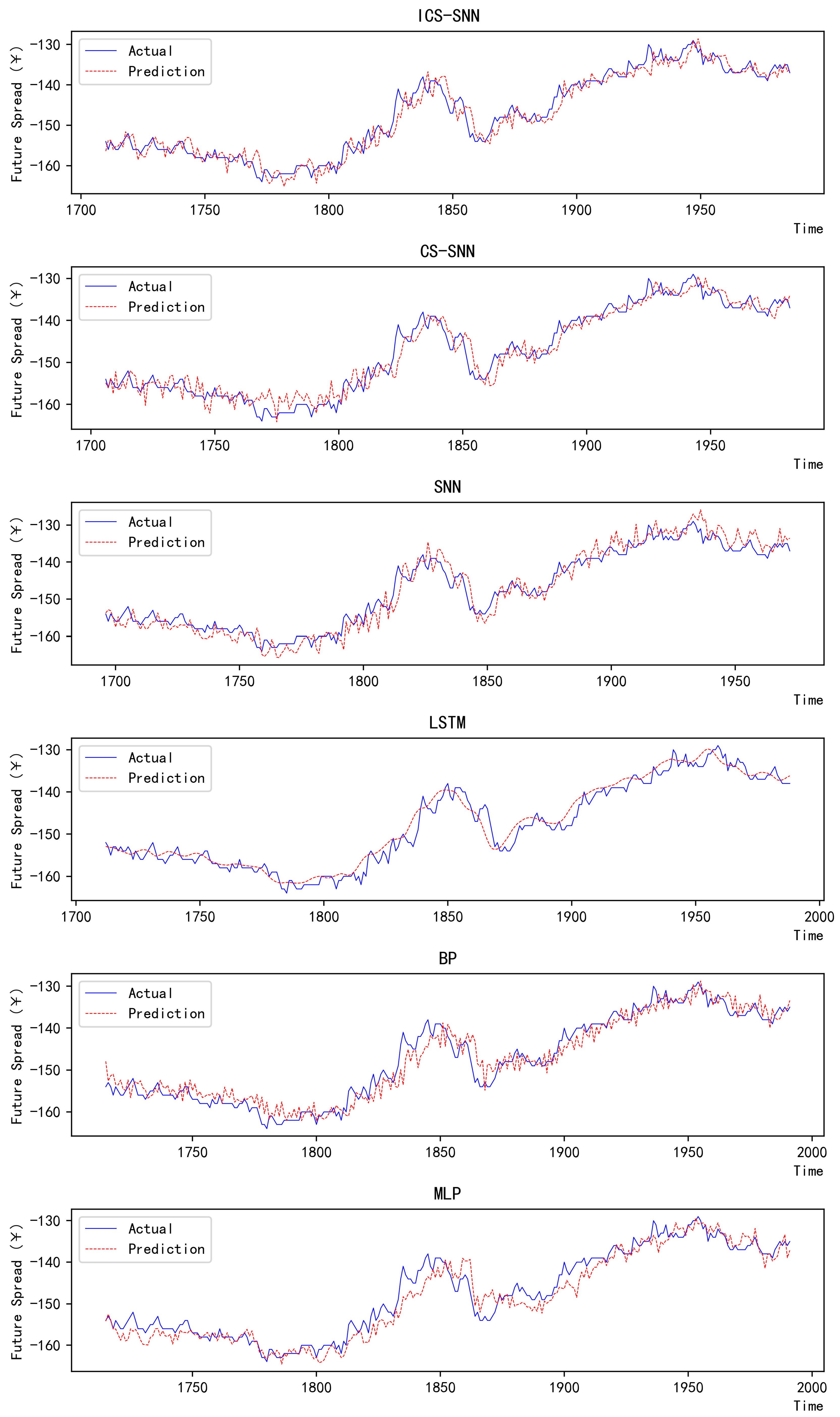
As the results show in Table 6 and Figure 8, MLP, as the first proposed model among the above models, has MAE, MSE, MAPE, and $R^2$ values of 3.0191, 16.9058, 0.0202, and 0.9717. Despite its simplicity—comprising only a few linear layers—MLP achieves reasonable performance in long-sequence modeling due to its straightforward architecture. And it is the most time-saving model among them.

BP is currently one of the most widely used neural network models. Its learning rule is to use the steepest descent method, which continuously adjusts the weights and thresholds of the network through BP to minimize the sum of squared errors of the network. Compared to MLP, BP has a better result in our experiments, and the values of the four metrics are 2.8884, 16.0640, 0.0192, and 0.9731.

Due to the unique design structure, LSTM is suitable for processing and predicting important events with very long intervals and delays in time series. Compared to the previous two models, its metrics were significantly better, being 2.6428, 13.2309, 0.0173, and 0.9779.

The hyperparameters of the SNN are chosen according to the following rules: with twice the number of iterations of ICS-SNN, adjust the hyperparameters based on experience, and then select the hyperparameter with the smallest metrics. The SNN model with manually tuned hyperparameters achieves MAE, MSE, MAPE, and R² values of 2.7351, 13.2958, 0.0184, and 0.9790, respectively. Although LSTM excels in capturing long-term dependencies, the ICS-SNN model surpasses it by leveraging optimized hyperparameters and temporal dynamics inherent to spiking neurons. The SNN has manually adjusted parameters, which means there is a long and tedious training process. Most numbers in people’s lives do not exceed two decimal places, so when researchers need to change the hyperparameter, they prefer to choose integers and numbers with no more than two decimal places. But the optimal solution is obviously randomly distributed, so there is a long way to go if we adjust the hyperparameters manually. Without hyperparameter optimization, SNNs demonstrate inferior performance compared to LSTM, highlighting the necessity of automated parameter tuning.

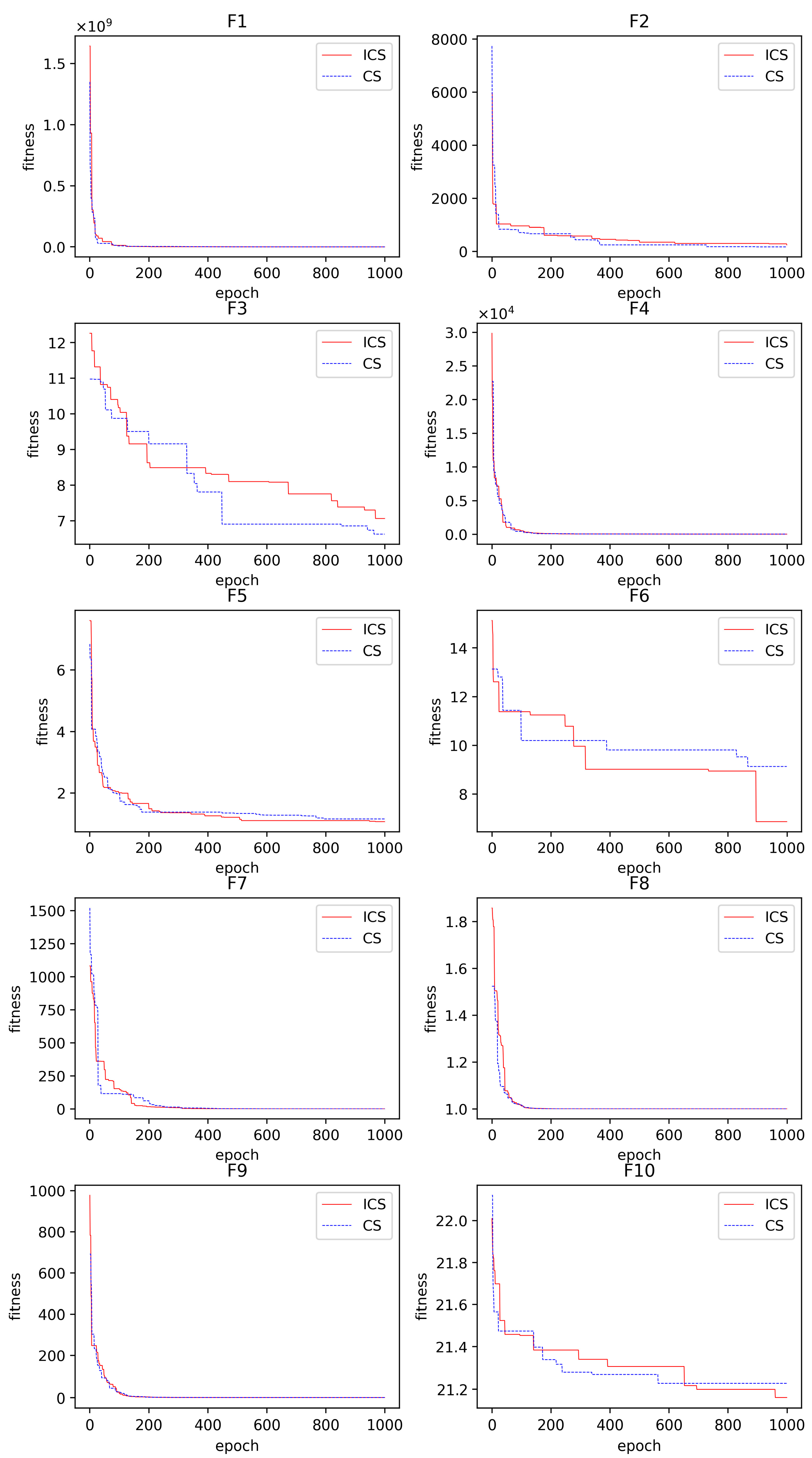
In order to see the improvement effect of ICS clearly, we conducted the CS-SNN experiments at the same time. The values of the four metrics are 2.4709, 11.2242, 0.0163, and 0.9812. The traditional CS algorithm can help the SNN achieve a small improvement. By automatically transforming hyperparameters, a greater chance of approaching the optimal solution is obtained.

The piecewise mapping in ICS ensures a more uniform initial population distribution, reducing the risk of local optima. Additionally, the adaptive discovery probability mimics natural cuckoo behavior, balancing exploration and exploitation. ICS-SNN obtains values of the four metrics of 2.3571, 10.4675, 0.0156, and 0.9822. Meanwhile, compared with SNN, ICS-SNN reduced MAE by 13.82%, MSE by 21.27%, and MAPE by 15.21%, and R^2 increased from 0.9790 to 0.9822. The final hyperparameter values of ICS-SNN, CS-SNN, and SNN are shown in

Table 7. The final hyperparameter values of ICS-SNN, CS-SNN, and SNN.

Model Name	Time Step	Neuron Number	Batch Size	Scaler Scope	Decay Rate	Threshold
ICS-SNN	11	952	1000	4.4328	0.5078	0.8413
CS-SNN	15	1809	1845	4.4615	0.6208	0.9459
SNN	25	1050	1500	5.0	0.55	1.0

. These hyperparameters work together on the results. The results obtained by individually modifying one parameter and simultaneously modifying multiple parameters may have significant differences.

Figure 9 is the pictorial result of 300 data to the reciprocal of actual and predicted values. It can be clearly seen from the figure that the two lines of ICS-SNN are closer together, which means its experimental results are the best among the six models.

Considering that the ICS-SNN model enhances its global search capability by introducing an ICS algorithm and uses RLIF to better process time series data, theoretically the model should be able to capture short-term market dynamics more effectively. Based on the 1-min K-line data we used, it is expected that the optimal prediction range of ICS-SNN may be concentrated within a few minutes to a few hours. In terms of long-term forecasting, although ICS-SNN performs well, the accuracy of predictions may decrease due to the complex factors affecting the financial market, especially unforeseeable macro events over a long time span.

Although the ICS-SNN model proposed in this study performed well in experimental environments, it still faces several challenges when applied in practical financial markets. Firstly, transaction costs directly affect the profitability of the strategy, especially in high-frequency trading scenarios where even small costs can accumulate into significant burdens. Secondly, liquidity constraints in the market may result in some predictions being unable to be executed, especially on low-liquidity assets. Finally, the issue of market delays cannot be ignored, as any delay may result in missing the best trading opportunity. Therefore, future research needs to focus more on how to overcome these practical obstacles to enhance the practical application value of the model.

5. Conclusions

This study proposes an ICS algorithm to help choose proper hyperparameters for SNNs in time series prediction.

Due to the simple structure, BP and MLP models’ results are the worst relatively. LSTM performs better than the original SNN, which demonstrates its powerful generalization ability. But when the hyperparameters are set correctly, the SNN can achieve effects comparable to LSTM. By changing the population initialization method, and improving the probability of host birds discovering eggs, we improved the efficiency of the cuckoo search algorithm. Then, this study also shows that SNNs have great potential in time series forecasting. And the ICS can help complete parameter selection automatically. The proposed algorithm significantly reduces researchers’ manual effort while maintaining high prediction accuracy. Extensive comparative experiments validate that the ICS-SNN model significantly reduces prediction errors (e.g., MSE) while maintaining computational efficiency.