Abstract
Laplacian controllability and observability of a consensus network is a widely considered topic in the area of multi-agent systems, complex networks, and large-scale systems. In this paper, this problem is addressed when the communication among nodes is described through a starlike tree topology. After a brief description of the mathematical setting of the problem adopted in a wide number of multi-agent systems engineering applications, some novel results are drawn based on node positions within the network only. The resulting methods are graphical and thus effective and exempt from numerical errors, and the final algorithm is provided to perform the analysis by machine computation. Several examples are provided to show the effectiveness of the algorithm proposed.
1. Introduction
In the last decades, the recent advancements of technology pushed a notable thrust of research into the area of complex systems made of an interconnection of locally interacting devices [1]. Within this framework, a significant research field is devoted to the ability of a node to drive the evolution of the team, thus giving rise to the topic of network controllability [2]. Network controllability has been largely investigated in the last decade, providing exciting and unexpected novel insights, motivated by a better understanding of complex self-organized systems operating and functioning [2].
A different yet related key property within the above framework of complex systems made of an interconnection of locally interacting devices is the ability of a single node or a small subset of nodes to infer global information of the network through an appropriate elaboration of local data, which is referred to as network observability [3]. Based on this concept of systems theory applied to complex networks, many fundamental algorithms have been designed to achieve a higher level of security and robustness such as, for example, monitoring the eventuality of edge faults or disconnections, compensating the detrimental effects of faults and errors on the global performances, or the ability of selecting sensor positioning within the network nodes to obtain the best global performances in network estimation problems [3].
Surprisingly, these two properties are strongly related from a mathematical perspective. Indeed, they are dual problems in the framework of systems theory [4], and they coincide in the case of a symmetric dynamical matrix. In the framework of multi-agent systems, this condition is a common feature when dealing with unweighted bidirectional communication, so that it is often verified.
For this reason, they are usually studied together, for the twofold goal of a deeper understanding of the functioning of complex networks of self-organized locally interacting nodes on one hand and design ability on the necessary sensors and actuators (in terms of number and positioning) to obtain some prescribed performance on the other [5,6]. Moreover, the above analysis allows us to gain a strong insight into the mechanism of controlling remote nodes, and many results can be extended, separately, for the analysis of controllability and observability of multiagent systems connected through a directed communication graph.
A common mathematical tool to properly analyze and understand complex network behavior and its features is the crossfield between systems theory and graph theory. Considering both of the above-mentioned structural properties, the spectrum and the eigenstructure of some graph-related matrices (such as the adjacency matrix or the Laplacian matrix) are the fundamental mathematical backbones [7,8], so that graph topology and its connection with spectral graph features has also been thouroghly investigated [5].
1.1. Literature Review
Controllability and observability are topics of interest to a broad community, and they have been studied over the years using several different tools, which has led to different approaches and results. In this Section, we review the main methodologies available in the literature for the analysis and design of controllability and observability of a network. In general, it is worth mentioning that this topic has been widely discussed in recent years, and the interested reader may also refer to the survey papers [9,10]. A careful and thorough overview of the approaches for the analysis of observability of network systems is [11].
One milestone paper that gave rise to the ideas of most of the further literature and approaches on this topic is [12]. In this paper, the authors introduce and motivate the controllability property of a multi-agent system, and they derive some basic fundamental results using several different approaches that have been largely investigated over the years.
One main direction stemming from this paper is the use of equitable partitions to detect uncontrollable graph topologies [13,14]. However, this method is proved to be only sufficient (and thus it provides only necessary conditions for controllability and observability). Moreover, the investigation of the existence of equitable partitions in large graphs may be difficult.
Other research directions exploring several different facets of controllability are the so-called structural controllability, namely the controllability analysis for almost all edge weights [15], and gramian-based controllability, where energy-based analysis is adopted to study the impact of control [16,17].
In paper [18], a brand new approach was introduced for the class of path and cycle graphs, considering the position of the control/measured nodes within the network, and necessary and sufficient conditions were derived based on simple modular algebra. This approach stimulated several reserch activities; in [19], the results of [18] were increasingly deepened and fully exploited.
The approach of [20] is based on the definition of minimal perfect critical set. This method is adequate to capture the minimum set of leaders for the controllability of undirected graphs, and it is applied to two different classes of bipartite networks, namely deterministic scale-free networks and Cayley trees.
In paper [21], path graphs and star graphs are considered, and the idea exploited is to also use second-order neighbors to improve controllability properties.
In order to summarize the above scientific literature on the topic of interest, we briefly report the different approaches and their limitations in Table 1.

Table 1.
Scientific literature summary.
1.2. Paper Contribution
In this paper, we extend the results of [18] to a wider class of graphs, namely the class of tree graphs having one node of degree larger than two, which are also known as starlike graphs [22,23] or spider graphs [24]. It is worth noting that, despite their simple and special topology, such a class of graphs has been recently very considered also among mathematicians for their interesting peculiar properties [22,25,26,27].
The contribution of this paper is to extend the results of [18] to gain a deeper insight into the more general case of acyclic graphs. More in detail, the contribution of this paper with respect to the above literature is threefold. First, we provide a complete characterization of node selection, in terms of minimal number and appropriate location within the network, of the class of starlike graphs. The main result is in terms of length of some sub-paths, so that the use of such results does not suffer from numerical errors when the number of participants grows, as opposed to most of the available results. As a second result, we provide deeper insights into the multiplicity of Laplacian eigenvalues of tree graphs, which is still an open problem within the mathematics community. Last, but not least, the third contribution is to achieve design ability in the construction of networks by connecting ’atom’ subgraphs and node selection to guarantee that the structural properties of network controllability and observability are ensured to hold.
Laplacian spectrum and eigenvector structure of tree graphs have been recently explored by the author also in [28,29]. We believe that the results achieved in this paper can be directly applied to several multi-agent systems and robotic network applications, as those provided for example in Section 2, and moreover they concur to have a thorough additional insight into the spectral properties of a Laplacian matrix of tree graphs.
In Table 2, we summarize the notation adopted along the paper.
Table 2.
Notation.
2. Problem Setting and Preliminary Results
In this Section, we introduce and then properly state the problem addressed in this paper.
Several distributed algorithms for multi-agent systems and robotic networks are designed according to the abstract mathematical framework described in the following, which we refer to as nearest-neighbor distributed averaging multi-agent system. Consider a set of N agents, each holding a continuous time scalar variable for each node with an update rule as Two neighbor agents are able to communicate between themselves and exchange their values (namely node i receives from node j and vice versa), and each node i sets its own input accoding to the agreed protocol:
Under this protocol, the evolution of the overall dynamics can be effectively described through an overall vector built as whose time update is compactly expressed by
denoting the topology of communication among agents.
Assume now that a subset of nodes , injecting an additional input to the agreed Protocol (1) with the intent of controlling the team evolution [12]. In this setting, the resulting system dynamics takes the following form:
with and . In the following, we refer to as the control nodes, or equivalently leader nodes.
Analogously, consider the case when it is desired to monitor the system evolution of (2), and the value of a subset of nodes is collected with the goal of reconstructing the whole system evolution. In such scenario, nodes are called observation nodes or measured nodes, and their values are exploited for supervision and surveillance of the whole system. In this case, the overall system dynamics is expressed by
with .
The above framework is widely adopted in several modern engineering applications in the area of distributed control systems and robotic networks [31,32,33].
Considering the above Setting (3), one main analysis is focused on the states that can be achieved through a suitable choice of , which are called controllable or reachable states and they constitute a subspace of of the state space called reachable subspace, denoted by . The reachable subspace can be obtained computing the image of the reachability matrix:
and if has full rank, System (3) is called completely controllable. In regard to the state estimation framework based on the knowledge of some measured nodes described by Equation (4), the system-theoretic analysis based on the intial state values that produce an identically zero measured vector, which are called unobservable states. The set of unobservable states is a subspace of that can be computed as the kernel of the observability matrix:
Remark 1.
Some multi-agent processes are better described by discrete updates of a local quantity, namely , where is called coupling factor and it should be chosen sufficiently small to keep the system stable [33], and analogously, in this case, one obtains the following system evolution:
with and B defined as in (3) in the case of control problems, oranalogously in the case of observability. However, it is possible to prove, and it is left to the reader, that the reachability analyses for (3) and (7) are equivalent, and the same holds for observability. For this reason, for the sake of coinciseness, we refer without loss of generality to (3) and (4).
2.1. Recent Engineering Applications
The above framework is adopted in several modern technological applications such as, for example, those reported below.
- Multi-robot systems and robotic networks [32]. The multi-agent setting (3) allows robot units of a team to coordinate and perform global actions without relying on a central supervisory device. Common global tasks are robot rendezvous (agents meeting at a common location), deployment (agents spreading out to cover an area), and formation control (agents keeping a predifined formation).
- Security and intrusion detection in cyber-physical systems, such as fault-tolerant distributed algorithm [34] and cyber-physical security [35]. In [34], controllability of (3) is the assumption to achieve almost sure resilient consensus. In [35], it is shown that observability, together with the absence of systems zeros, is required to achieve security.
- Wireless Sensor Networks. The multi-agent setting is employed to address fundamental issues in wireless sensor networks, such as synchronization [36], or averaging algorithms [37].
- Automotive Networking and UAV formation control. The above multi-agent setting is widely employed to achieve formation control through distributed algorithms in vehicle networks and UAVs [38,39,40].
- Electrical Power Systems. With the evolution of the electric grid toward a smart grid, the multi-agent setting is widely adopted to tackle new emerging challenges such as load balancing, fault detection and isolation, demand response, and others [41,42]. Cyber-physical attacks in power networks using the above models are studied in [43].
2.2. Problem Statement
Inspired by the applications discussed in the previous paragraph, we are now ready to state the problem that we address in the rest of this paper. However, considering the discussion in the previous Section 1.1 regarding paper contributions, we provide two problem statements that are equivalent between themselves, considering the two facets (mathematical/engineering) of the same investigation. Here, we offer the genuine statement as it is presented in [12]. After a brief discussion on the spectral methods for the analysis of reachability and observability, we rephrase the problem in a mathematical fashion, which is related to the eigenstructure investigation afforded in [22,23,24,25,26,27,28,29,30,31,32,33,34,35,36,37,38,39,40,41,42,43,44].
Problem Statement 1.
Considering the significance of the above properties in the analysis of dynamical systems, several results and technical tools have been developed to obtain an accurate and thorough investigation of a dynamical system. Among the others, the Popov–Belevich–Hautus polynomial approach is one of the most adopted methods for its effectiveness [4]. Its use in the context of Laplacian-based multi-agent system provides fundamental tools for such analysis.
In view of the investigation based on spectral methods reported in Appendix A.1 the previous Problem Statement can be equivalently rephrased in terms of zero pattern of each eigenvactor, thus translating the problem in a more mathematical fashion. More precisely, the controllability and observability condition is equivalent to solving the following problem.
Problem Statement 2.
Given a starlike tree graph , we provide a complete characterization of the zero-nonzero pattern of each eigenvector of the Laplacian matrix of , together with the multiplicity for each .
3. Laplacian Controllability and Observability of Starlike Graphs
In this Section, we derive a set of results which constitute the complete theoretical characterizaton of node selection for controllability and observability for the class of starlike tree graphs.
It is worth mentioning that the Laplacian eigentructure of starlike graphs has been widely studied also by mathematicians in the recent years for their peculiar features. For example, contrary to path graphs, which always have simple Laplacian eigenvalues, in starlike graphs Laplacian eigenvalue multiplicity may range from 1 to . Consider the two starlike graphs in Figure 1. Graph depicted in Figure 1a has , so that , and at least three nodes must be selected to achieve reachability. Conversely, graph in Figure 1b has , and hence all eigenvalues are simple. Considering the problem of interest, the minimum number of nodes necessary to achieve complete controllability and observability in case of Figure 1a is three in the first case (and hence more than half of the nodes constituting the whole network), while in the case of Figure 1b, it is possible to have complete reachability and observability by properly selecting only one node. We show later that the differences between the two graphs are even more evident; indeed, in Figure 1a, such nodes must be chosen joudiciously, while in Figure 1b reachability and observability is achieved by choosing any node of the network.
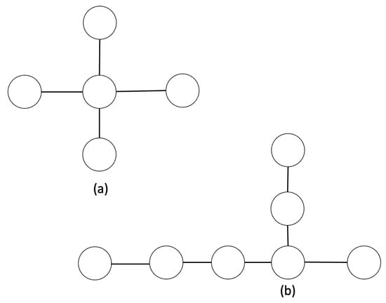
Figure 1.
Examples showing large differences in eigenvalue multiplicities. Graph (a) has and it is controllable by selecting at least three leaf nodes, Graph (b) has all simple eigenvalues and it is controllable by any single node.
3.1. Starlike Trees with Simple Eigenvalues—Preliminary Results
We start the analysis focusing on starlike graphs having simple eigenvalues only. It is worth mentioning that for trees, integer Laplacian eigenvalues larger than one are necessarily simple [45]. In contrast to this, Laplacian eigenvalue is often present in the tree Laplacian spectrum, and its occurrence and multiplicity have been longly studied by mathematicians [46].
In the following sections of the paper, we adopt the labeling described next. The central node, namely the only node having degree larger than two, is usually denoted by subindex c and it is put as first entry of vector . Then, , are the values of nodes starting from the neighbor of the central node to the pendant node of Branch 1. The other branches are labeled sequentially and they follow the same ordering logic.
Considering this labeling, the general form of a starlike graph is
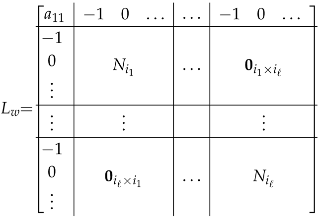 where is the number of branches starting from the central node. Matrices are some fundamental structured matrices for the forthcoming analysis, and they are defined and characterized as follows.
We refer to an external branch of p nodes as the path with one grounded external node, with grounded Laplacian matrix:
and to an internal branch of q nodes as
Figure 2 shows an example of an external branch of two nodes (upper side of the Figure 2) and one internal branch of two nodes. The associated grounded Laplacians are
and
The grounded nodes are graphically denoted with a double circle.
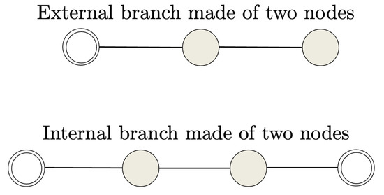
Figure 2.
Example of external branch (above) and internal branch (below). They constitute the basic elements of the proposed graph reduction technique proposed in this paper. Grey nodes are related to nonzero eigenvector components, white double-circled nodes are associated to zero eigenvector components.
Laplacian spectrum of path graphs, of the two class of matrices , , and their relations are reported in Appendix A.2.
Considering again the example depicted in Figure 1, it is easy to compute from (A7) and from (A8) and . Moreover, it is left to the reader to verify that are also the eigenvalues of using Equation (A5) for and and finally that the eigenvalues of are indeed coicident with those of (but the zero eigenvalue).
A first simple yet important result follows. It is focused on an eigenvector condition that ensures controllability/observability from any node, namely having a nonzero value in each entry. It turns out a special condition on eigenvalues, namely that only eigenvalues associated to subpaths of the branches can be unreachable.
3.2. Starlike Eigenvalues Associated with Nowhere Zero Eigenvactors
One interesting and surprising result follows. It basically states that loss of reachability and observability may occur only for those eigenvalues characterizing the grounded Laplacians of the constitutive branch paths. It implies that integer eigenvalues different from one have nowhere zero eigenvectors, and hence they can be controlled by any node.
Proposition 1.
We let be the spectrum of a star graph , and define , where, for each branch, . Any eigenvalue belonging to the set (where − stands for set difference) is always reachable and observable from any node.
Proof.
We compute an eigenvector with one zero component. Consider the eigenvalue equation built on a Laplacian matrix as (8) and an eigenvector having zero in any position, namely
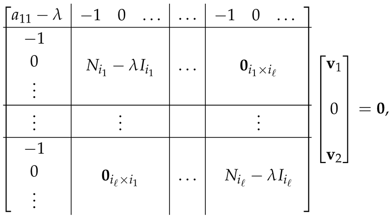 where with , and both and are nonzero. Exploiting (13), one has
where is the starlike graph obtained by removing the subpath of length from the sth branch. Last equation implies that, in such a case of eigenvector with one zero component, must be necessarily also an eigenvalue of , and by property of Proposition A2, must be also eigenvalue of . Since the ordering of the branches is generic, this proof applies to any branch, and the statement follows. □
where with , and both and are nonzero. Exploiting (13), one has
where is the starlike graph obtained by removing the subpath of length from the sth branch. Last equation implies that, in such a case of eigenvector with one zero component, must be necessarily also an eigenvalue of , and by property of Proposition A2, must be also eigenvalue of . Since the ordering of the branches is generic, this proof applies to any branch, and the statement follows. □
4. Zero-Nonzero Pattern of Eigenvectors Associated to
As per the previous result, we start the investigation by considering subpaths of incresing dimension. In this Section, we thoroughly discuss the case . The corresponding matrix is the scalar value , so that its only eigenvalue is .
It is worth noting that the eigenstructure of for tree graphs is widely considered in the literature from the seminal work of [45] to our days [47], and it is still a debated topic.
In the following, we provide a description of the two different conditions that make a Laplacian eigenvalue of a star-like graph .
The first stage is the reduction in the star-like graph to its core, namely a subgraph obtained by reducing the branches to a ’core’ of few nodes by reducing from the pendant node each branch as described analitically in Appendix B, or graphically, as depicted in Figure 3. Figure 4 shows an example of reduction to a core.
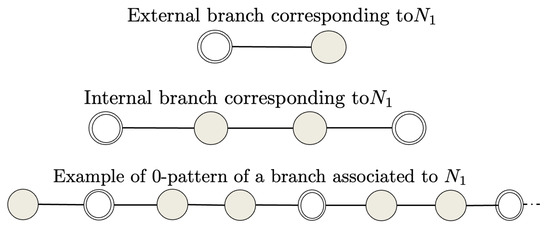
Figure 3.
Zero pattern associated to . The upper and middle branches constitute the basic elements of the proposed graph reduction technique in case of (external and internal, respectively); the lowest is an example of zero-nonzero pattern of eigenvector starting from one leaf, put on the left. Grey nodes are related to nonzero eigenvector components, double-circled white nodes are associated to zero eigenvector components.
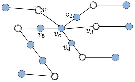
Figure 4.
Example of a graph reduction to a core related to , related to . The core graph is the subgraph made of .
We now focus on a generic core to find conditions under which the considered Laplacian admits as eigenvalue, or eventually not. A thorough investigation by simulation on all possible core structures provided two different topology conditions coherent with at the central node, which are briefly described in the following. We denote by , ,… the values afforded by the neighbors of , ,… at the opposite position with respect to applying the reduction technique described in Appendix B. The two conditions consistent with at the central node are as follows:
- (R1)
- If any of the branch reductions show , then at least one other should show analogously , othewise is not an eigenvalue of . This is the case when . In this case, we denote by r the number of branches whose reduction satisfies , .
- (R2)
- If all , then the eigenvalue condition (see, e.g., Equation (A9)) evaluated at the central node has solution if and only if only one and all the other , for any . In this case, the solution is , and whenever the above condition holds, in this case always.
To provide an example, we come back to the graph depicted in Figure 4. It is possible to see that node evaluation matches the condition , so we fall in (R2). However, in this case, two nodes have (namely and ), so that (R2) is not satisfied, and this means that is not an eigenvalue of . Indeed, in this case, it is possible to verify that the eigenvalue equation computed at the central node does not hold.
Figure 5 shows some graphs with few differences from Figure 4, namely and , but they both have in their spectrum and different multiplicity. Consider Figure 5a; in this case, Condition (R2) is fully met. As for Figure 5b, it matches Condition with , so that . The two branches with white nodes satisfy the eigenvalue equation for zero node values only.
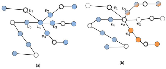
Figure 5.
Example of starlike graphs whose reduction leads to a core that falls into, respectively, Cases R1 (a) and R2 (b).
Node Selection for Reachability and Observability of
Considering all the above analysis and results, and specifically the eigenspace dimension and zero/nonzero structure, it is now easy to deduce the node selection rule to achieve reachability and observability in the case of .
For the above reason, the following procedure is more suited in the case of complex graphs, with hundreds or more nodes. In the following procedure, we denote the eigenvector of by the symbol (in general, denotes the eigenvector associated to ).
In the next Section, stemming from the experience on , we easily develop an algorithm for a general and we derive an overall algorithm with Algorithm 1 as one of its blocks.
| Algorithm 1 Node selection for controllability and observability. Case . |
|
5. Zero-Nonzero Pattern of Eigenvectors Associated to Any of
Interestingly, the above conditions on can be extended in the general case of any .
We start this generalization by an example regarding ; then, we describe the general procedure that extends conditions (R1)–(R2) to the general case of of .
Consider the two graphs depicted in Figure 6. They represent the generalization to of the two graphs discussed in Figure 5, and they are related, respectively, to Conditions (R1) and (R2) for , namely . They are obtained by replacing the branches characterizing (see Figure 3) with those of (Figure 7) and by adding one neighbor node to each branch around the central node .
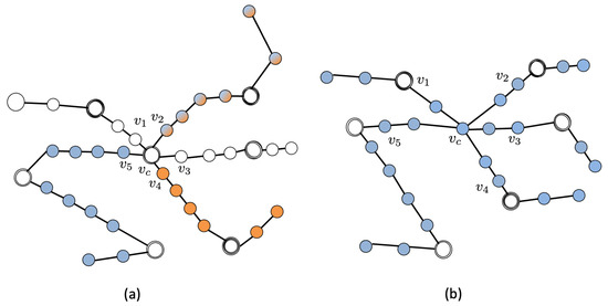
Figure 6.
Example of extension of Cases R1 (a) and R2 (b) for eigenvalues of , with .
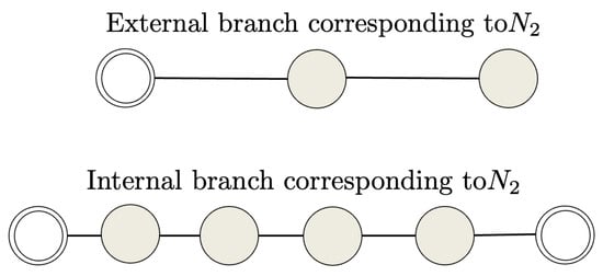
Figure 7.
External and internal branches associated to . They constitute the basic elements of the proposed graph reduction technique in case of . Grey nodes are related to nonzero eigenvector components, double-circled white nodes are associated to zero eigenvector components.
Starting from the above consideration, we are now ready to generalize rules (R1)–(R2) as follows.
We let , . As a first step, we reduce the graph to the core based on the basic elements depicted in Figure 8. Then, is an eigenvalue of the considered starlike graph if one of the following two conditions hold:
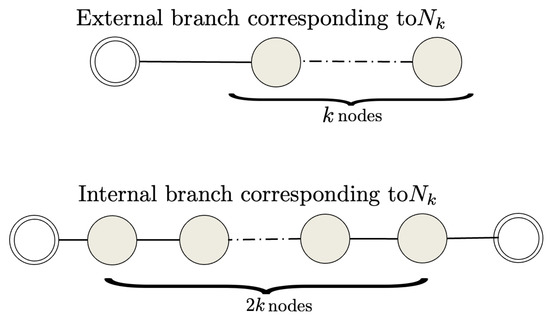
Figure 8.
External and internal branches associated to . They are the basic elements of the proposed graph reduction technique in case of . Grey nodes are related to nonzero eigenvector components, double-circled white nodes are associated to zero eigenvector components.
- (R1)
- The reduction related to of at least two branches provides . If r denotes the number of branches whose reduction satisfies , (), then has multiplicity .
- (R2)
- After reducing the graph, the core is made of branches all of length k but only one of length . In this case, and .
However, eigenvectors related to Condition (R2) can be found only if , so that its search is limited to the length of the smallest branch; conversely, eigenvectors as in (R2) can be found until there are two possible branches, and its search must be performed up to the largest-but-one branch. In this latter case, ordering the branches such that for , when , then the eigenvector components relative to the branches ,…, are necessarily zero.
This allows us to state a generalization of Algorithm 1 to any k. In the following, we state Algorithm 2 that allows us to get the for , being the shortest branch, and then we provide Algorithm 3, which is the adaption of Algorithm 1 for the remaining branches for .
| Algorithm 2 Node selection for controllability and observability. Case , . |
|
When , only one case is possible, and the algorithm is simplified as follows.
| Algorithm 3 Node selection for controllability and observability. Case ,. |
|
The above algorithms must be exploited together, sequentially, as shown in the flow chart in Figure 9. Indeed, the set of control/observation nodes needed to achieve controllability and observability is the union of the set of control/observation nodes of each eigenvalue so that, for ,
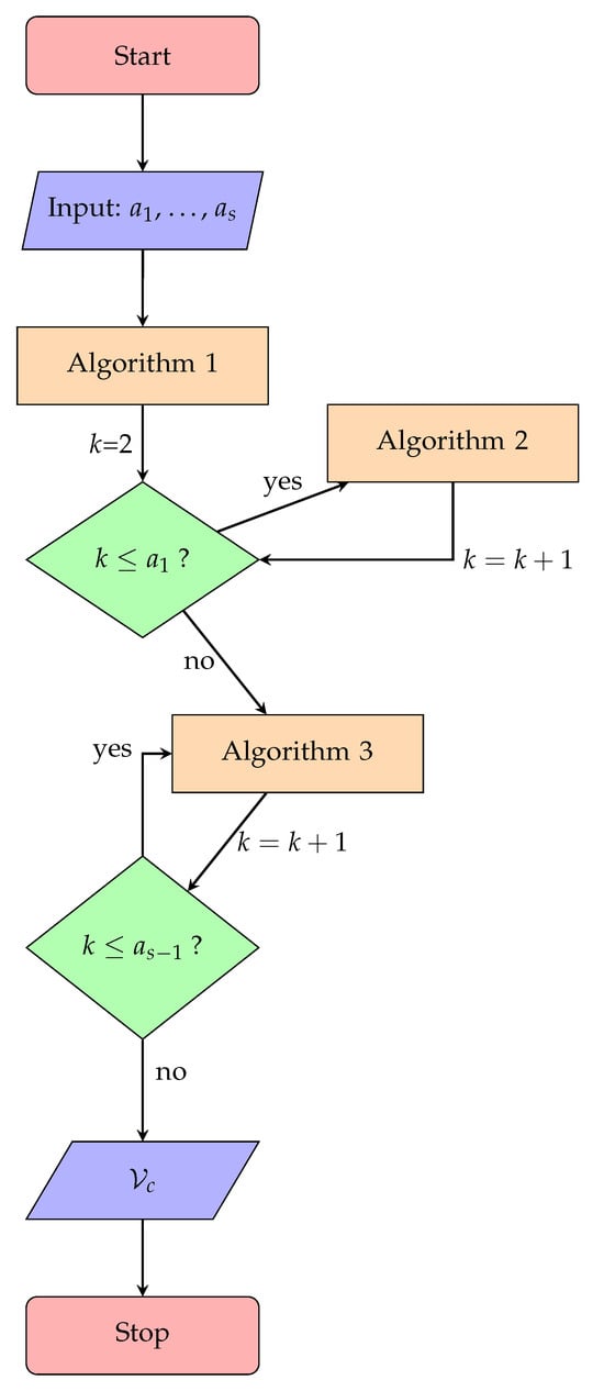
Figure 9.
Flowchart describing the overall algorithm, merging Algorithms 1–3.
Discussion on the Main Features of the Proposed Algorithm
One main peculiarity of the node selection preocedure that follows is that it does not require any theoretical knowledge in dynamical systems or spectral graph theory. It can be effectively used by non-experts in the field of control theory, whenever this property is required to achieve a high performance (e.g., security algorithms).
A second fundamental advantage of the following procedure is that it is purely graphical so that it does never incur numerical errors, as opposite to most algorithms in this field. Consider that Matrices (5)/(6) have the structure of Vandermonde matrices, so that numerical errors arise starting from relatively small dimensions (less than 10), and the computation based on (5)/(6) can be effective only for networks of few nodes. Also, investigations through the PBH criterion, namely Equation (A1)/(A2), require rank evaluations so that they are adequate for graphs up to 20–30 nodes.
6. An Illustrative Example
In this Section, we practice with the overall algorithm through an illustrative example, which also puts in evidence the effectiveness of the proposed approach when dealing with large graphs and hence in the framework of complex networks.
Consider the starlike tree graph depicted in Figure 10, which is made of 6 branches and 37 nodes, and it corresponds to . Nodes are labeled according to the convention adoptedalong the paper, namely the center is labeled as Node 1 and then the branches are numbered from the center to the leaves. They are ordered starting from the shortest to the longest one.
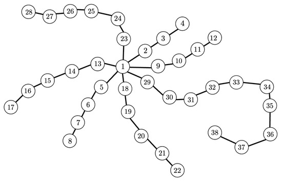
Figure 10.
Sketch of the starlike graph considered in the illustrative example.
In the following, we discuss the graphical result of the algorithm, as shown in Figure 11. Colored nodes are related to nonzero eigenvector components obtained by making all the possible reductions, namely for , and for each applying Algorithms 1, 2, or 3. The color pink is associated to reductions in , light green to , and purple to . All other possible reductions do not match either (R1) or (R2), so the related eigenvalues are not eigenvalues of .
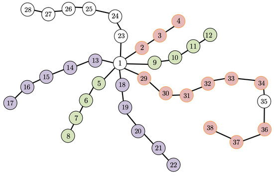
Figure 11.
Graphical result of the algorithm applied to the starlike graph in Figure 10.
In the following, we report the multiplicity of the eigenvalues of , , together with the set of control/observation nodes that are selected according to Algorithms 2 and 3.
while all the other for are not eigenvalues of .
Considering that the above sets are disjoint, a set of control/observation nodes to achieve controllability must contain one node for each of the above set, and an example of a minimal set is .
7. Conclusions
In this paper, the Laplacian controllability and observability of a consensus network with a starlike tree topology is considered and thoroughly analyzed. First, the problem setting is introduced, together with the description of some modern engineering applications that motivate the analysis, and the problem statement is then provided. Next, a thorough investigation of the zero-nonzero pattern of Laplacian eigenvectors is performed, starting from and then extending the criterion to any . Some novel results are drawn based on node positions within the network only. Based on these results, three algorithms are provided to solve three basic partial problems, and the overall algorithm is explained through a block diagram. The resulting methods are graphical and thus effective and exempt from numerical errors, and a final algorithm is provided to perform the analysis by machine computation, showing numerical robustness and the important feature of dealing with large scale networks and complex systems.
The results achieved so far and described thoroughly in this paper are promising, and the proposed approach can be extended to other, more general topology classes.
Funding
This research received no external funding.
Data Availability Statement
The datasets generated for this study are available on request from the corresponding author.
Conflicts of Interest
The author declares no conflicts of interest.
Appendix A. Spectral Methods for Controllability and Observability Analysis
Appendix A.1. Popov–Belevich–Hautus (PBH) Method
The Popov–Belevich–Hautus polynomial approach for controllability and observability analysis is one of the most adopted methods for its effectiveness [4]. Its use in the context of Laplacian-based multi-agent system provides fundamental tools for such analysis.
Proposition A1.
We now specialize this criterion considering some peculiarities of (3) and (4). Considering that the Laplacian matrix is symmetric, all its eigenvalues are real and semi-simple, so that for any [30].
Condition (A1) is violated if there exist a nonzero vector such that
and this is equivalent to say that
In turn, this means that there should exist an eigenvector with zero value along all the components corresponding to the control nodes. Whenever this condition holds, we call , an unreachable eigenvalue and eigenvector. Complete system reachability requires that such eigenvectors do not exist.
Remark A1
(Minimal set of control nodes for complete controllability). From the above discussion, the number of control/measured nodes must be larger or at least equal to the maximum multiplicity of eigenvectors . Moreover, for the second condition of (A3), it is fundamental to understand the zero-nonzero pattern of each eigenvector.
It is possible to derive an analogous condition for observability, requiring that
Namely, there should exist an eigenvector with zero components along the observation nodes. Also, in this case, when this condition holds, , are called unobservable eigenvalue and eigenvector, and complete system observability requires that such eigenvectors do not exist.
Clearly, in the case of observability, analogous considerations hold. However, considering again the symmetry of matrix , a system is reachable through a set of control nodes if and only if it is observable from the same set of measured nodes, and for this reason we deduce that the controllability problem and the observability problem are indeed equivalent for systems evolving with Laplacian dynamics, as (3) and (4).
Appendix A.2. Laplacian Spectrum of Path Graphs, of the Two Class of Matrices Ni, Mj, and Their Relations
In the following, we characterize the Laplacian spectrum of path graphs, of the two class of matrices , , and their relations. Laplacian spectrum and eigenstructure of path graphs have been widely considered and studied. Here, we briefly offer the formulas that characterize it for the sake of completeness. We let be a Path graph, namely we assume that and . The complete set of eigenvalues of the Laplacian of can be written as
and associated eigenvectors
Considering the two class of matrices and , their eigenvalues and eigenvectors are, respectively, [18]
and
For the sake of clarity of the rest of the paper, we remark that there are some relations among the eigenvalues and eigenvectors of , , and .
Proposition A2.
For any , , the following relations hold:
Proof.
In regard to , through standard determinant computation using the Laplace formula, it is possible to obtain
so that plus the zero eigenvalue. As for , by comparing (A7) with (A5), it is possible to prove by direct computation that all the eigenvalues of are contained in the spectrum of , and it is possible to obtain them by selecting from (A5) the values corresponding to the odd values, from 1 to , of (A5). □
Appendix B. Graph Reduction to the Core Graph
Consider the Laplacian eigenvalue equation applied to each node, namely:
where is the degree of node i and the ith component of an eigenvector associated to (also called valuation of an eigenvector affording [45]).
Applying Equation (A9) with to the first branch, starting from one pendant node and moving to the center according to the usual labeling, one has
and this amounts to saying that the eigenvector associated to must satisfy the evaluation , with being a nonzero value, thus showing the zero value in positions as depicted in Figure 3.
References
- Herrera, M.; Pérez-Hernández, M.; Kumar Parlikad, A.; Izquierdo, J. Multi-agent systems and complex networks: Review and applications in systems engineering. Processes 2020, 8, 312. [Google Scholar] [CrossRef]
- Liu, Y.Y.; Slotine, J.J.; Barabási, A.L. Controllability of complex networks. Nature 2011, 473, 167–173. [Google Scholar] [CrossRef]
- Liu, Y.Y.; Slotine, J.J.; Barabási, A.L. Observability of complex systems. Proc. Natl. Acad. Sci. USA 2013, 110, 2460–2465. [Google Scholar] [CrossRef]
- Antsaklis, P.J.; Michel, A. Linear Systems; Birkhauser: Basel, Switzerland, 1997. [Google Scholar]
- Leitold, D.; Vathy-Fogarassy, Á.; Abonyi, J. Controllability and observability in complex networks–the effect of connection types. Sci. Rep. 2017, 7, 151. [Google Scholar] [CrossRef]
- Doostmohammadian, M.; Rabiee, H.R. On the observability and controllability of large-scale IoT networks: Reducing number of unmatched nodes via link addition. IEEE Control Syst. Lett. 2020, 5, 1747–1752. [Google Scholar] [CrossRef]
- Yan, G.; Tsekenis, G.; Barzel, B.; Slotine, J.J.; Liu, Y.Y.; Barabási, A.L. Spectrum of controlling and observing complex networks. Nat. Phys. 2015, 11, 779–786. [Google Scholar] [CrossRef]
- Stigter, J.; Joubert, D.; Molenaar, J. Observability of complex systems: Finding the gap. Sci. Rep. 2017, 7, 16566. [Google Scholar] [CrossRef]
- Knorn, S.; Chen, Z.; Middleton, R.H. Overview: Collective control of multiagent systems. IEEE Trans. Control Netw. Syst. 2015, 3, 334–347. [Google Scholar] [CrossRef]
- Chen, F.; Ren, W. On the control of multi-agent systems: A survey. Found. Trends® Syst. Control 2019, 6, 339–499. [Google Scholar] [CrossRef]
- Montanari, A.N.; Aguirre, L.A. Observability of network systems: A critical review of recent results. J. Control. Autom. Electr. Syst. 2020, 31, 1348–1374. [Google Scholar] [CrossRef]
- Rahmani, A.; Ji, M.; Mesbahi, M.; Egerstedt, M. Controllability of multi-agent systems from a graph-theoretic perspective. SIAM J. Control Optim. 2009, 48, 162–186. [Google Scholar] [CrossRef]
- Martini, S.; Egerstedt, M.; Bicchi, A. Controllability analysis of multi-agent systems using relaxed equitable partitions. Int. J. Syst. Control Commun. 2010, 2, 100–121. [Google Scholar] [CrossRef]
- Aguilar, C.O.; Gharesifard, B. Almost equitable partitions and new necessary conditions for network controllability. Automatica 2017, 80, 25–31. [Google Scholar] [CrossRef]
- Mousavi, S.S.; Haeri, M.; Mesbahi, M. On the structural and strong structural controllability of undirected networks. IEEE Trans. Autom. Control 2017, 63, 2234–2241. [Google Scholar] [CrossRef]
- Pasqualetti, F.; Zampieri, S.; Bullo, F. Controllability metrics, limitations and algorithms for complex networks. IEEE Trans. Control Netw. Syst. 2014, 1, 40–52. [Google Scholar] [CrossRef]
- Pasqualetti, F.; Zhao, S.; Favaretto, C.; Zampieri, S. Fragility limits performance in complex networks. Sci. Rep. 2020, 10, 1774. [Google Scholar] [CrossRef] [PubMed]
- Parlangeli, G.; Notarstefano, G. On the reachability and observability of path and cycle graphs. IEEE Trans. Autom. Control 2011, 57, 743–748. [Google Scholar] [CrossRef]
- Liu, X.; Ji, Z. Controllability of multiagent systems based on path and cycle graphs. Int. J. Robust Nonlinear Control 2018, 28, 296–309. [Google Scholar] [CrossRef]
- Dai, L. Minimum leader selection for controllability of undirected graphs with leader–follower framework. IET Control Theory Appl. 2023, 17, 505–515. [Google Scholar] [CrossRef]
- Chao, Y.; Ji, Z. Necessary and sufficient conditions for multi-agent controllability of path and star topologies by exploring the information of second-order neighbours. IMA J. Math. Control Inf. 2021, 38, 1–14. [Google Scholar] [CrossRef]
- Lepović, M.; Gutman, I. No starlike trees are cospectral. Discret. Math. 2002, 242, 291–296. [Google Scholar] [CrossRef]
- Nakatsukasa, Y.; Saito, N.; Woei, E. Mysteries around the graph Laplacian eigenvalue 4. Linear Algebra Its Appl. 2013, 438, 3231–3246. [Google Scholar] [CrossRef]
- Weisstein, E.W. Spider Graph. MathWorld–A Wolfram Web Resource. 2025. Available online: https://mathworld.wolfram.com/SpiderGraph.html (accessed on 1 March 2025).
- Akbari, S.; van Dam, E.; Fakharan, M. Trees with a large Laplacian eigenvalue multiplicity. Linear Algebra Its Appl. 2020, 586, 262–273. [Google Scholar] [CrossRef]
- Pei-Duo, Y.; Tan, C.W. Unraveling the Viral Spread of Misinformation: Maximum-Likelihood Estimation and Starlike Tree Approximation in Markovian Spreading Models. IEEE Trans. Signal Process. 2025, 73, 446–461. [Google Scholar]
- Yu, P.D.; Zheng, L.; Tan, C.W. Contagion source detection by maximum likelihood estimation and starlike graph approximation. In Proceedings of the 2024 58th Annual Conference on Information Sciences and Systems (CISS), Princeton, NJ, USA, 13–15 March 2024; pp. 1–6. [Google Scholar]
- Parlangeli, G. Laplacian Eigenvalue Allocation Through Asymmetric Weights in Acyclic Leader-Follower Networks. IEEE Access 2023, 11, 126409–126419. [Google Scholar] [CrossRef]
- Parlangeli, G. A Distributed Algorithm for Reaching Average Consensus in Unbalanced Tree Networks. Electronics 2024, 13, 4114. [Google Scholar] [CrossRef]
- Horn, R.; Johnson, C. Matrix Analysis; Cambridge University Press: Cambridge, UK, 2012. [Google Scholar]
- Mesbahi, M.; Egerstedt, M. Graph Theoretic Methods in Multiagent Networks; Princeton University Press: Princeton, NJ, USA, 2010. [Google Scholar]
- Bullo, F.; Cortés, J.; Martínez, S. Distributed Control of Robotic Networks; Applied Mathematics Series; Princeton University Press: Princeton, NJ, USA, 2009. [Google Scholar]
- Bullo, F. Lectures on Network Systems, 1.6 ed.; Kindle Direct Publishing: Seattle, WA, USA, 2022. [Google Scholar]
- Shang, Y. Resilient vector consensus over random dynamic networks under mobile malicious attacks. Comput. J. 2024, 67, 1076–1086. [Google Scholar] [CrossRef]
- Pasqualetti, F.; Dorfler, F.; Bullo, F. Control-theoretic methods for cyberphysical security: Geometric principles for optimal cross-layer resilient control systems. Control Syst. IEEE 2015, 35, 110–127. [Google Scholar] [CrossRef]
- Swain, A.R.; Hansdah, R. A model for the classification and survey of clock synchronization protocols in WSNs. Ad Hoc Netw. 2015, 27, 219–241. [Google Scholar] [CrossRef]
- Oliveira, L.M.; Rodrigues, J.J. Wireless Sensor Networks: A Survey on Environmental Monitoring. J. Commun. 2011, 6, 143–151. [Google Scholar] [CrossRef]
- Khan, S.; Hussain, I.; Khattak, M.I. Consensus based formation control of multiple UAVs. J. Inf. Commun. Technol. Robot. Appl. 2020, 11, 31–37. [Google Scholar]
- Meng, Q.; Kasis, A.; Polycarpou, M.M. Integrated Attitude-Position Formation Control of Multiple Vehicles on SE(3) With Individual Objectives. IEEE Trans. Aerosp. Electron. Syst. 2025. [Google Scholar] [CrossRef]
- Liang, X.; Ge, S.S.; Li, D. Coordinated tracking control of multi agent systems with full-state constraints. J. Frankl. Inst. 2023, 360, 12030–12054. [Google Scholar] [CrossRef]
- Farhangi, H. The path of the smart grid. IEEE Power Energy Mag. 2009, 8, 18–28. [Google Scholar] [CrossRef]
- Molzahn, D.K.; Dörfler, F.; Sandberg, H.; Low, S.H.; Chakrabarti, S.; Baldick, R.; Lavaei, J. A survey of distributed optimization and control algorithms for electric power systems. IEEE Trans. Smart Grid 2017, 8, 2941–2962. [Google Scholar] [CrossRef]
- Pasqualetti, F.; Dörfler, F.; Bullo, F. Cyber-physical attacks in power networks: Models, fundamental limitations and monitor design. In Proceedings of the IEEE Conference on Decision and Control and European Control Conference, Orlando, FL, USA, 12–15 December 2011; pp. 2195–2201. [Google Scholar]
- Saito, N.; Woei, E. Tree simplification and the ‘plateaux’phenomenon of graph Laplacian eigenvalues. Linear Algebra Its Appl. 2015, 481, 263–279. [Google Scholar] [CrossRef]
- Grone, R.; Merris, R.; Sunder, V.S. The Laplacian spectrum of a graph. SIAM J. Matrix Anal. Appl. 1990, 11, 218–238. [Google Scholar] [CrossRef]
- Barik, S.; Lal, A.; Pati, S. On trees with Laplacian eigenvalue one. Linear Multilinear Algebra 2008, 56, 597–610. [Google Scholar] [CrossRef]
- Wang, Z.; Chen, Q.Q.; Guo, J.M.; Li, X.M. A relation between multiplicity of 1 as a Laplacian eigenvalue and induced matching numbers in trees. Discret. Math. 2025, 348, 114401. [Google Scholar] [CrossRef]
Disclaimer/Publisher’s Note: The statements, opinions and data contained in all publications are solely those of the individual author(s) and contributor(s) and not of MDPI and/or the editor(s). MDPI and/or the editor(s) disclaim responsibility for any injury to people or property resulting from any ideas, methods, instructions or products referred to in the content. |
© 2025 by the author. Licensee MDPI, Basel, Switzerland. This article is an open access article distributed under the terms and conditions of the Creative Commons Attribution (CC BY) license (https://creativecommons.org/licenses/by/4.0/).