Utilizing a Bounding Procedure Based on Simulated Annealing to Effectively Locate the Bounds for the Parameters of Radial Basis Function Networks

Abstract

Radial basis function (RBF) networks are an established parametric machine learning tool which has been extensively utilized in data classification and data fitting problems. These specific machine learning tools have been applied in various scientific areas, such as problems in physics, chemistry, and medicine, with excellent results. A two-step technique is usually used to adjust the parameters of these models, which is in most cases extremely effective. However, it does not effectively explore the value space of the network parameters and often results in parameter stability problems. In this paper, the use of a bounding technique that explores the value space of the parameters of these networks using intervals generated by a procedure based on the Simulated Annealing method is recommended. After finding a promising range of values for the network parameters, a genetic algorithm is applied within this range of values to more effectively adjust its parameters. The new method was applied on a wide range of classification and regression datasets from the relevant literature and the results are reported in the current manuscript.

1. Introduction

A wide range of practical problems can be considered as classification or regression problems. Such problems occur in areas such as physics [1,2], astronomy [3,4], chemistry [5,6], medicine [7,8], economics [9,10], etc. A machine learning tool commonly used to tackle such problems is the radial basis function (RBF) network, expressed as the following function:

$$R\left(\overrightarrow{x}\right)=\sum _{i=1}^k{w}_i\varphi \left(∥\overrightarrow{x}-\overrightarrow{c_i}∥\right)$$

(1)

In this equation, the following definitions are used for the symbols:

• The vector $\overrightarrow{x}$ represents the input pattern with d number of features.
• The parameter k stands for the number of weights of the network. These weights are represented by the values $w_i,i=1,\dots ,k$.
• The vectors $\overrightarrow{c_i},i=1,\dots ,k$ represent the so-called centers of the network.
• The function $\varphi \left(x\right)$ commonly is a Gaussian function with the following definition:

  $$\varphi \left(x\right)=exp\left(-{\displaystyle \frac{{\left(x-c\right)}^2}{{\sigma }^2}}\right)$$

  (2)

A typical plot of the Gaussian function for $c=0,\sigma =1$ is depicted in Figure 1. From this graph it is deduced that the Gaussian RBF decreases regarding the distance from c. The parameters c and $\sigma$ can be estimated using the K-Means algorithm, introduced by MacQueen [11]. The training error of an RBF network is defined as

$$E\left(R\left(\overrightarrow{x}\right)\right)=\sum _{i=1}^M{\left(R\left(\overrightarrow{x_i}\right)-y_i\right)}^2$$

(3)

where $\left(\overrightarrow{x_i},y_i\right),i=1,\dots ,M$ represents the training set of the objective problem and the values $y_i$ are the expected outputs for every pattern $\overrightarrow{x_i}$.

RBF networks have been incorporated in various cases, such as face recognition [12], solutions of differential equations [13,14], stock prediction [15], robotics [16,17], network security [18,19], etc.

Due to the widespread use of these networks, several papers have been presented in recent years that study their basic characteristics. For example, Benoudjit et al. [20] presented a discussion on kernel widths in RBF networks. Similarly, Oyang et al. [21] presented a novel method for the estimation of the kernel density. Moreover, Ros et al. [22] proposed an automatic method for the initialization of the parameters of RBF networks. Furthermore, a variety of pruning techniques have also been proposed [23,24], used to efficiently reduce the number of processing units of RBF networks in order to avoid the overfitting problem. Also, for the effective training of RBF networks a variety of methods has been proposed in the recent literature, such as the incorporation of genetic algorithms [25,26], usage of the Particle Swarm Optimization (PSO) method [27,28], the usage of methods based on Differential Evolution [29], etc. Furthermore, since there has been an extremely large spread of parallel programming techniques in recent decades, publications have also appeared that exploit such techniques for the efficient and fast training of the above networks [30,31].

In most cases, RBF networks are trained using a two-stage technique. In the first stage, the centers and variances are estimated using the K-means technique. In the second stage, a linear system is solved to find the weights of the Gaussian units. Although the above procedure is extremely fast, it cannot effectively explore the value space for the network parameters and in many cases numerical stability problems occur when solving the linear system. This paper proposes a three-stage method for the efficient training of RBF networks. In the first stage, an initial estimate of the centers and fluctuations of the RBF network is made using the K-means technique. Subsequently, an interval generation method based on Simulated Annealing [32] is used to efficiently identify the optimal interval of network parameter values. The creation of the value interval is performed within a value interval that is based on the initial estimate of the network parameters made in the first phase of the method. In the last phase of the proposed technique, a genetic algorithm is used to train the parameters of the machine learning model within the optimal value interval resulting from the second stage of the method.

The rest of this article is divided as follows: In Section 2 the proposed method is presented in detail; in Section 3 the used datasets as well as the conducted experiments are presented; and finally, in Section 4 some conclusions are discussed as well as some guidelines for improvements of the current work.

2. Method Description

In this section, a detailed presentation of the three phases of the proposed technique is made using appropriate algorithms.

2.1. The First Phase of the Proposed Method

A typical diagram of an RBF network is depicted in Figure 2. Every RBF network with k weights has the following sets of parameters:

• A series of vectors $\overrightarrow{c_i},i=1,\dots ,k$ that represent the centers of the network. Each center has d values.
• Each Gaussian unit has an additional parameter ${\sigma }_i$ that corresponds to the variance of this unit.
• The set of output weights $\overrightarrow{w}$ with k values.

Provided that the input vector $\overrightarrow{x}$ has d values, the total number of parameters of an RBF network is calculated as

$$n=(d+2)\times k$$

(4)

For the determination of initial values for the centers and variances, the K-means algorithm is utilized here and it is presented in Algorithm 1.

Algorithm 1 Description of the K-means algorithm.

Initialization (a) The input of the algorithm is the points $x_i,i=1,\dots ,M$ belonging to the train set of the objective problem, (b) Define as k the number of centers. (c) Set $S_j=\left\{\right\}$, $j=1,\dots ,k$. Repeat (a) For each point $x_i,i=1,\dots ,M$ do i. Set $j^{*}={\mathrm{argmin}}_{m=1}^k\left\{D\left(x_i,c_m\right)\right\}$. The index $j^{*}$ denotes the nearest center for point $x_i$. The function $D(x,y)$ represents the Euclidean distance. ii. Set $S_{j^{*}}=S_{j^{*}}\cup \left\{x_i\right\}$. iii. End For (b) For every center $c_j,j=1\dots k$ do i. Set $M_j$ as the number of points in $S_j$ ii. Update the center $c_j$ with the following equation: $$c_j={\displaystyle \frac{1}{M_j}}\sum _{x_i\in S_j}{x}_i$$ (c) End For The algorithm terminates when $c_j$ no longer changes The output of the algorithm are the $\overrightarrow{c_i},i=1,\dots ,k$ centers and the corresponding variances ${\sigma }_i,i=1,\dots ,k$

When this process is finished, the vector $\overrightarrow{z}$ with the calculated parameters is formed using the function calculateZ(), described in Algorithm 2.

Algorithm 2 The algorithm used for the calculation of the initial set of parameters for the RBF network.

Function calculateZ($\overrightarrow{c},\overrightarrow{\sigma },w_0)$ Inputs: The initial calculated values for centers $\overrightarrow{c},$ the initial values for variances $\overrightarrow{\sigma }$ and a positive value $w_0$. Set $l=1$ For $i=1,\dots ,k$ do (a) For $j=1,\dots ,d$ do i. Set $z_l=c_{i,j}$ ii. Set $l=l+1$ (b) End For End For For $i=1,\dots ,k$ do (a) Set $z_l={\sigma }_i$ (b) Set $l=l+1$ End For For $i=1,\dots ,k$ do (a) Set $z_l=w_0$, where $w_0$ a positive double precision number. (b) Set $l=l+1$ End For Return the vector $\overrightarrow{z}$. End function

The layout of the vector $\overrightarrow{z}$ is outlined in Figure 3. In this layout, the initial values of the centers are entered at the beginning of the vector, then the initial values for the variances are entered, and finally the initial values for the network weights.

2.2. The Second Phase of the Proposed Method

In the second phase of the algorithm, the value interval for the network parameters is constructed using a technique based on Simulated Annealing. Simulated Annealing is an optimization procedure used in a variety of cases, such as resource allocation [33], portfolio problems [34], energy problems [35], biology [36], etc. The algorithm starts from a large value of a factor called temperature, which is gradually decreased. For large values of temperature, the algorithm performs a wide exploration of the search space, and at low values it focuses around some minimum of the objective function. The Simulated Annealing variant used here minimizes interval functions denoted as

$$f\left(x\right)=\left[f_{\min }\left(x\right),f_{\max }\left(x\right)\right]$$

(5)

Also, in order to compare two intervals $a=\left[a_1,a_2\right]$ and $b=\left[b_1,b_2\right]$, the operator $D(a,b)$ is incorporated with the following definition:

$$D(a,b)=\left\{\begin{array}{cc}\mathrm{TRUE},\hfill & a_1<b_1\mathrm{OR}\left(a_1=b_1\mathrm{AND}{a}_2<b_2\right)\hfill \\ \mathrm{FALSE},\hfill & \mathrm{otherwise}\hfill \end{array}\right.$$

(6)

The method used below assumes that there are value intervals for the network parameters. The main steps of the method used in the second phase are shown as a procedure in Algorithm 3. The calculation of the functional values for such value intervals is performed using Algorithm 4.

The algorithm starts from an initial value interval, which is based on the result of the first phase of the overall process. At each iteration it generates random value intervals that are close to the current value interval. If a value interval with a smaller functional value than the current one is presented, it is accepted; otherwise it will be accepted with a probability that is high for large temperature values and decreases significantly as the temperature value drops. This means that the algorithm makes a wide exploration of the search space for high temperature values and centers around some minimum as the temperature value decreases.

Algorithm 3 The main steps of the proposed Simulated Annealing variant.

Function simanMethod $\left(\overrightarrow{z},F,T_0,r_T,N_{\mathrm{eps}},a\right)$ Inputs: The vector $\overrightarrow{z}$ with the initial set of parameters, the limit factor $F>1$, the initial temperature $T_0$, the reduction factor for temperature $r_T,r_T>0,r_T<1$, the number of samples taken at every iteration denoted as $N_{\mathrm{eps}}$ and $a>0$ the perturbation factor. Construct the bound vectors $L^{*},R^{*}$ using the vector $\overrightarrow{z}$ of the first phase as follows: $$\begin{array}{ccccc}{L}_i^{*}& =& -F\times z_i& ,& i=1,\dots ,n\\ R_i^{*}& =& F\times z_i& ,& i=1,\dots ,n\end{array}$$ The parameter F is a positive number greater than 1 and is used as a limiting factor for the network parameters. Set $k=0$ Set $x_b=\left[L^{*},R^{*}\right],y_b=\mathrm{fitness}\left(L^{*},R^{*},N_s\right)$. This function utilizes the function fitness() outlined in Algorithm 4. Set $x_c=x_b,y_c=y_b$ For $i=1,\dots ,N_{\mathrm{eps}}$ do (a) Produce a random sample $x_t=\left(L_t,R_t\right)$ using the procedure of Algorithm 5 using as inputs to the function the interval $x_c=\left[L_c,R_c\right]$ and the double precision number a. (b) Set $y_t=\mathrm{fitness}\left(L_t,R_t,N_s\right)$ which calls the function provided in Algorithm 4. (c) If $D\left(y_t,y_c\right)=\mathrm{TRUE}$ then Set $x_c=x_t,y_c=y_t$ (d) Else Set $x_c=x_t$ with probability $min\left\{1,exp\left(-{\displaystyle \frac{f_t-f_c}{T_k}}\right)\right\}$ (e) End if (f) If $D\left(x_c,x_b\right)=\mathrm{TRUE}$ then Set $x_b=x_c,y_b=y_c$ End For Set $T_{k+1}=T_k{r}_T$ Set $k=k+1$. If $T_k\le ϵ$ stop and return $x_b=\left[L_b,R_b\right]$ as the best located interval of bounds. Go to step 5. End function

Algorithm 4 The algorithm used to calculate the function value for intervals of parameters.

function fitness $\left(L,R,N_s\right)$ Create the set $T=\left\{r_1,r_2,\dots ,r_{N_s}\right\}$ with $N_s$ random samples in $\left[L,R\right]$. Set $E_{\min }=\infty ,E_{\max }=-\infty$ For $i=1,\dots ,N_s$ do (a) Create the RBF network $R_i\left(\overrightarrow{x}\right)$ using as parameter set the corresponding sample $r_i\in T$. (b) Calculate the training error $f_{R_i}={\sum }_{j=1}^M{\left(R_i\left(\overrightarrow{x_j}\right)-y_j\right)}^2$ for the training set of the objective problem. (c) If $f_{R_i}\le E_{\min }$ then $E_{\min }=f_{R_i}$ (d) If $f_{R_i}\ge E_{\max }$ then $E_{\max }=f_{R_i}$ End For Return the interval $\left[E_{\min },E_{\max }\right]$. End function

Algorithm 5 The sampling function used in the Simulated Annealing algorithm.

Function sample $\left(L,R,a\right)$ For $i=1,\dots ,n$ do (a) Set $m=L_i+{\displaystyle \frac{R_i-L_i}{2}}$ (b) Set $L_i^x=L_i+a{r}_1\left(m-L_i\right)$, where $r_1\in [0,1]$ a random value. (c) Set $R_i^x=R_i-a{r}_2\left(R_i-m\right)$, where $r_2\in [0,1]$ a random value. End For Return $x=\left[L^x,R^x\right]$ the located interval. End function

2.3. The Final Phase of the Proposed Method

In the last phase of the proposed procedure, a genetic algorithm is executed to train the RBF network. The training is performed within the optimal value interval identified in the previous phase of the proposed procedure. The main steps of the proposed genetic algorithm are shown in Algorithm 6.

Algorithm 6 The final phase of the proposed method.

Procedure finalPhase $\left(N_c,N_g,p_s,p_m,\left[L_b,R_b\right]\right)$ Inputs: Number of chromosomes $N_c,$ number of generations $N_g$, selection rate $p_s$, mutation rate $p_m$, the bounds the bounds $\left[L_b,R_b\right]$ of previous phase. Initialize the chromosomes $g_i,i=1,\dots ,N_c$ as random vectors inside the bounds $\left[L_b,R_b\right]$ of the second phase of the suggested algorithm. Set $k=0$ For $i=1,\dots ,N_c$ do (a) Create the RBF network $R_i\left(\overrightarrow{x}\right)$ using as parameters the chromosome $g_i$. (b) Calculate the corresponding fitness value $f_i={\sum }_{j=1}^M{\left(R_i\left(\overrightarrow{x_j}\right)-y_j\right)}^2$ End For Selection procedure. The $p_s\times N_c$ best chromosomes with the lowest fitness values are copied intact to the next generation. The remaining chromosomes will be replaced by new chromosomes produced in crossover and mutation procedure. Crossover procedure. During the application of crossover, pairs of chromosomes are chosen from the current population with tournament selection. For every pair $(z,w)$ of parents two new chromosomes $\tilde{z}$ and $\tilde{w}$ are will be produced using the following equations: $$\begin{array}{ccc}\hfill \widetilde{z_i}& =& a_i{z}_i+\left(1-a_i\right)w_i\hfill \\ \hfill \widetilde{w_i}& =& a_i{w}_i+\left(1-a_i\right)z_i\hfill \end{array}$$ (7) where $i=1,\dots ,n$ and $a_i$ are randomly selected values with $a_i\in [-0.5,1.5]$ [37]. Mutation procedure. For every element of each chromosome a random number $r\in [0,1]$ is produced. This element will be altered randomly when $r\le p_m$. Set $k=k+1$ If $k<N_g$ then go to step 3. Obtain the best chromosome $g_b$ from the genetic population, with the lowest fitness value. Create the corresponding RBF network $R_b\left(\overrightarrow{x}\right)$ Apply $R_b\left(\overrightarrow{x}\right)$ to the corresponding test set and measure the associated test error and Terminate. End procedure

3. Experiments

A series of classification and regression datasets from various websites was incorporated to test the proposed method and to measure its reliability. The datasets used in the conducted experiments were downloaded from the following online databases:

• The UCI database: https://archive.ics.uci.edu/ (accessed on 26 March 2025) [38]
• The Keel website: https://sci2s.ugr.es/keel/datasets.php (accessed on 26 March 2025) [39].
• The Statlib URL: https://lib.stat.cmu.edu/datasets/ (accessed on 26 March 2025).

3.1. Experimental Datasets

In the conducted experiments, the following classification datasets were used:

• The Alcohol dataset, used in various experiments regarding alcohol consumption [40].
• The Appendicitis dataset [41].
• The Australian dataset, used in various bank transactions [42].
• The Balance dataset, used in a series of psychological experiments [43].
• The Circular dataset, which is an artificial dataset.
• The Cleveland dataset, which is a medical dataset [44,45].
• The Dermatology dataset, obtained from various dermatology problems [46].
• The Hayes-Roth dataset [47].
• The Heart dataset, which is a medical dataset regarding heart diseases [48].
• The HeartAttack dataset, used in the prediction of heart attacks.
• The HouseVotes dataset, that contains data from congressional voting in the USA [49].
• The Ionosphere dataset, obtained from various experiments in the ionosphere [50,51].
• The Liverdisorder dataset, which is a medical dataset [52,53].
• The Lymography dataset [54].
• The Mammographic dataset, which is a medical dataset [55].
• The Parkinsons dataset, used for the detection of Parkinson’s disease [56,57].
• The Phoneme datasets, obtained from various sound experiments.
• The Pima dataset, a medical dataset used in the diabetes studies [58].
• The Popfailures dataset, related to measurements from climate model simulations [59].
• The Regions2 dataset, which is a medical dataset [60].
• The Saheart dataset, which is a medical dataset about heart disease [61].
• The Segment dataset, related to issues regarding image processing [62].
• The Sonar dataset, related to sonar signals [63].
• The Spiral dataset, which is an artificial dataset.
• The StatHeart dataset, a medical dataset related to heart disease.
• The Student dataset, derived from various experiments in schools [64].
• The Transfusion dataset [65].
• The WDBC dataset, which is a medical dataset about the detection of cancer [66].
• The Wine dataset, related to the detection of the quality of wines [67,68].
• The EEG dataset, which is obtained from various EEG measurements [69,70]. The cases Z_F_S, Z_O_N_F_S, ZO_NF_S, and ZONF_S were used from this dataset.
• The ZOO dataset, used for animal classification [71].

Moreover, the following regression datasets were obtained for the conducted experiments:

• The Abalone dataset, that contains data related to the age of abalones [72].
• The Airfoil dataset, obtained from NASA [73].
• The Auto dataset, used to estimate the fuel consumption in cars.
• The Baseball dataset, related to the estimation of the salary of baseball players.
• The BK dataset, used for the prediction of points in basketball games [74].
• The BL dataset, used in some electricity experiments.
• The Concrete dataset, derived from civil engineering [75].
• The Dee dataset, used for the estimation of the price of electricity.
• The Housing dataset, used to estimate the price of houses [76].
• The Friedman database [77].
• The FA dataset, which is related to fat measurements.
• The FY dataset, that contains data regarding fruit flies.
• The HO dataset, that was derived from the STATLIB repository.
• The Laser dataset, used in various laser experiments.
• The MB dataset, derived from smoothing methods in statistics.
• The Mortgage dataset, that contains economic measurements.
• The NT dataset [78].
• The Plastic dataset, that contains measurements from experiments conducted related to pressure in plastics.
• The PY dataset [79].
• The PL dataset, downloaded from the STATLIB repository.
• The Quake dataset, related to the estimation of the strength of earthquakes.
• The SN dataset, that contains measurements about trellising and pruning.
• The Stock dataset, which is an economic dataset about the prediction of the price of stocks.
• The Treasury dataset, which contains economic measurements.

3.2. Experimental Results

The code used in the experiments was implemented in the C++ programming language and a machine equipped with 128 GB RAM running Debian Linux was utilized in the conducted experiments. The code was written with the assistance of the freely available GlobalOptimus optimization environment, that can be downloaded from https://github.com/itsoulos/GlobalOptimus (accessed on 12 April 2025). Each experiment was executed 30 times and the average classification error was measured for the classification datasets and the average regression error was measured for the regression datasets. The classification error was computed using the following equation:

$$E_C\left(R\left(x\right)\right)=100\times {\displaystyle \frac{{\sum }_{i=1}^K\left(\mathrm{class}\left(R\left(x_i\right)\right)-y_i\right)}{K}}$$

(8)

where the set $T=\left\{x_i,y_i\right\},i=1,\dots ,K$ stands for the test set of the current problem and $R\left(x\right)$ is the RBF model. The regression error was calculated through the following equation:

$$E_R\left(R\left(x\right)\right)={\displaystyle \frac{{\sum }_{i=1}^K{\left(R\left(x_i\right)-y_i\right)}^2}{K}}$$

(9)

The values for the parameters of the proposed method are mentioned in

Table 1. The values for the experimental parameters.

Parameter	Meaning	Value
$w_0$	Initial values for the weights	100.0
F	Scale factor used in the initialization	10.0
$T_0$	Initial temperature	${10}^6$
$ϵ$	Small value used in comparisons	${10}^{-6}$
a	Perturbation factor	0.001
$N_s$	Number of samples used in the fitness calculation	100
$N_{eps}$	Number of samples taken in Simulated Annealing	100
$N_c$	Number of chromosomes	500
$N_g$	Maximum number of allowed generations	200
$p_s$	Selection rate	0.1
$p_m$	Mutation rate	0.05

. The selection of values for the experimental parameters was performed in such a way that there was a compromise between the speed and reliability of the proposed methodology. In the following tables, that describe the experimental results, the following notation is used:

• The column Dataset represents the name of the objective problem.
• The column BFGS denotes the application of the BFGS optimization method [80] in the training of a neural network [81,82] with 10 processing nodes.
• The column ADAM stands for the incorporation of the ADAM optimizer [83] to train an artificial neural network with 10 processing nodes.
• The column NEAT represents the usage of the NEAT method (NeuroEvolution of Augmenting Topologies) [84].
• The column RBF-KMEANS stands for the usage of the original two-phase method to train an RBF network with 10 processing nodes.
• The column GENRBF represents the incorporation of the method proposed in [85] to train an RBF network with 10 processing nodes.
• The column Proposed denotes the usage of the proposed method to train an RBF network with 10 processing nodes.
• The row Average represents the average classification or regression error.
• The row W-average denotes the average classification error for all datasets and for each method. In this average, each individual classification error was multiplied by the number of patterns for the corresponding dataset.

The results from the application of the previously mentioned machine learning methods to the classification datasets are depicted in

Table 2. Experimental results for the classification datasets using the series of machine learning methods adopted here. The numbers in cells represent average classification error as measured on the corresponding test set.

Dataset	BFGS	ADAM	NEAT	RBF-KMEANS	GENRBF	Proposed
Alcohol	41.50%	57.78%	66.80%	49.38%	52.45%	31.28%
Appendicitis	18.00%	16.50%	17.20%	12.23%	16.83%	15.27%
Australian	38.13%	35.65%	31.98%	34.89%	41.79%	21.00%
Balance	8.64%	7.87%	23.14%	33.42%	38.02%	12.95%
Cleveland	77.55%	67.55%	53.44%	67.10%	67.47%	50.82%
Circular	6.08%	19.95%	35.18%	5.98%	21.43%	4.19%
Dermatology	52.92%	26.14%	32.43%	62.34%	61.46%	36.13%
Hayes-Roth	37.33%	59.70%	50.15%	64.36%	63.46%	33.54%
Heart	39.44%	38.53%	39.27%	31.20%	28.44%	15.33%
HeartAttack	46.67%	45.55%	32.34%	29.00%	40.48%	18.52%
HouseVotes	7.13%	7.48%	10.89%	6.13%	11.99%	3.74%
Ionosphere	15.29%	16.64%	19.67%	16.22%	19.83%	7.39%
Liverdisorder	42.59%	41.53%	30.67%	30.84%	36.97%	27.92%
Lymography	35.43%	29.26%	33.70%	25.50%	29.33%	20.64%
Mammographic	17.24%	46.25%	22.85%	21.38%	30.41%	17.21%
Parkinsons	27.58%	24.06%	18.56%	17.41%	33.81%	15.35%
Phoneme	15.58%	29.43%	22.34%	23.32%	26.29%	16.62%
Pima	35.59%	34.85%	34.51%	25.78%	27.83%	23.59%
Popfailures	5.24%	5.18%	7.05%	7.04%	7.08%	4.80%
Regions2	36.28%	29.85%	33.23%	38.29%	39.98%	25.54%
Saheart	37.48%	34.04%	34.51%	32.19%	33.90%	29.64%
Segment	68.97%	49.75%	66.72%	59.68%	54.25%	40.83%
Sonar	25.85%	30.33%	34.10%	27.90%	37.13%	18.25%
Spiral	47.99%	48.90%	50.22%	44.87%	50.02%	22.52%
StatHeart	39.65%	44.04%	44.36%	31.36%	42.94%	19.52%
Student	7.14%	5.13%	10.20%	5.49%	33.26%	5.11%
Transfusion	25.84%	25.68%	24.87%	26.41%	25.67%	24.59%
Wdbc	29.91%	35.35%	12.88%	7.27%	8.82%	5.00%
Wine	59.71%	29.40%	25.43%	31.41%	31.47%	7.71%
Z_F_S	39.37%	47.81%	38.41%	13.16%	23.37%	3.16%
Z_O_N_F_S	65.67%	78.79%	77.08%	48.70%	68.40%	46.77%
ZO_NF_S	43.04%	47.43%	43.75%	9.02%	22.18%	3.63%
ZONF_S	15.62%	11.99%	5.44%	4.03%	17.41%	1.79%
ZOO	10.70%	14.13%	20.27%	21.93%	33.50%	4.50%
Average	32.98%	33.60%	32.46%	28.39%	34.64%	18.67%
W-average	32.01%	34.97%	34.32%	30.13%	34.73%	20.21%

, and for the regression datasets the results are presented in

Table 3. Experimental results for regression datasets. Numbers in cells represent average regression error as calculated on the corresponding test set.

Dataset	BFGS	ADAM	NEAT	RBF-KMEANS	GENRBF	Proposed
Abalone	5.69	4.30	9.88	7.37	9.98	5.10
Airfoil	0.003	0.005	0.067	0.27	0.121	0.004
Auto	60.97	70.84	56.06	17.87	16.78	9.68
Baseball	119.63	77.90	100.39	93.02	98.91	86.19
BK	0.28	0.03	0.15	0.02	0.023	0.153
BL	2.55	0.28	0.05	0.013	0.005	0.0002
Concrete	0.066	0.078	0.081	0.011	0.015	0.006
Dee	2.36	0.630	1.512	0.17	0.25	0.16
Housing	97.38	80.20	56.49	57.68	95.69	18.70
Friedman	1.26	22.90	19.35	7.23	16.24	1.45
FA	0.426	0.11	0.19	0.015	0.15	0.019
FY	0.22	0.038	0.08	0.041	0.041	0.077
HO	0.62	0.035	0.169	0.03	0.076	0.01
Laser	0.015	0.03	0.084	0.03	0.075	0.003
MB	0.129	0.06	0.061	2.16	0.41	5.49
Mortgage	8.23	9.24	14.11	1.45	1.92	0.14
NT	0.129	0.12	0.33	8.14	0.02	0.007
PL	0.29	0.117	0.098	2.12	0.155	0.023
Plastic	20.32	11.71	20.77	8.62	25.91	2.29
PY	0.578	0.09	0.075	0.012	0.029	0.019
Quake	0.42	0.06	0.298	0.07	0.79	0.036
SN	0.40	0.026	0.174	0.027	0.027	0.024
Stock	302.43	180.89	12.23	12.23	25.18	1.53
Treasury	9.91	11.16	15.52	2.02	1.89	0.51
Average	26.43	19.62	12.84	9.19	12.28	5.48

.

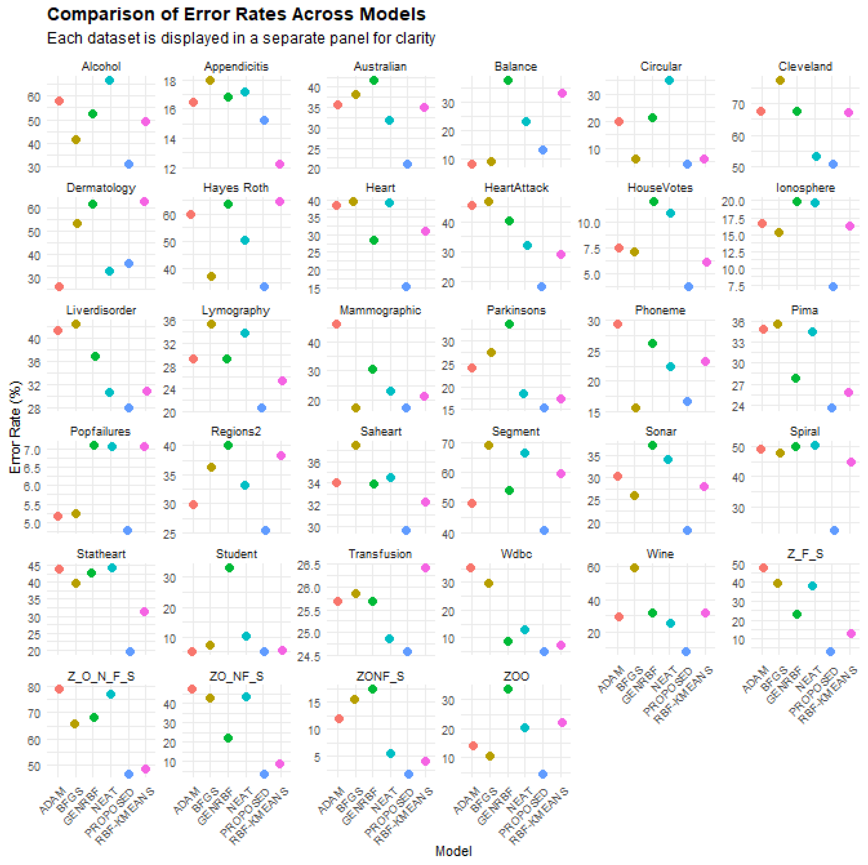
Table 2 presents the error rates of the various machine learning models (BFGS, ADAM, NEAT, RBF-KMEANS, GENRBF, proposed) on the different classification datasets. Each row corresponds to a dataset, while each column represents the error rate of a specific model. These values indicate the percentage of incorrect predictions, with lower values reflecting better performance. The last row of the table includes the average error rates for each model. Statistical analysis of the data reveals significant insights. The proposed model exhibits the lowest average error rate (18.67%) compared to the other models, establishing it as the optimal choice based on the table. Conversely, the other models demonstrate higher average error rates, with GENRBF showing the highest average error (34.64%). Additionally, significant variations in error rates across datasets are observed. For instance, on the “Circular” and “ZONF_S” datasets, the proposed model outperforms others, with very low error rates (4.19% and 1.79%, respectively). Conversely, on datasets like “Cleveland”, the NEAT model shows a lower error rate (53.44%) compared to the proposed model (50.82%). Notably, in certain datasets, the performance of the proposed model is significantly inferior to other models. For example, on the “Alcohol” and “Z_F_S” datasets, the proposed model exhibits much higher error rates compared to other models. This indicates that while the proposed model generally has the lowest average error rate, its performance may not be consistent across all datasets. In conclusion, the proposed model emerges as the best general choice for minimizing error rates, though its evaluation depends on the characteristics of each dataset. The performance differences among models highlight the need for careful model selection depending on the application.

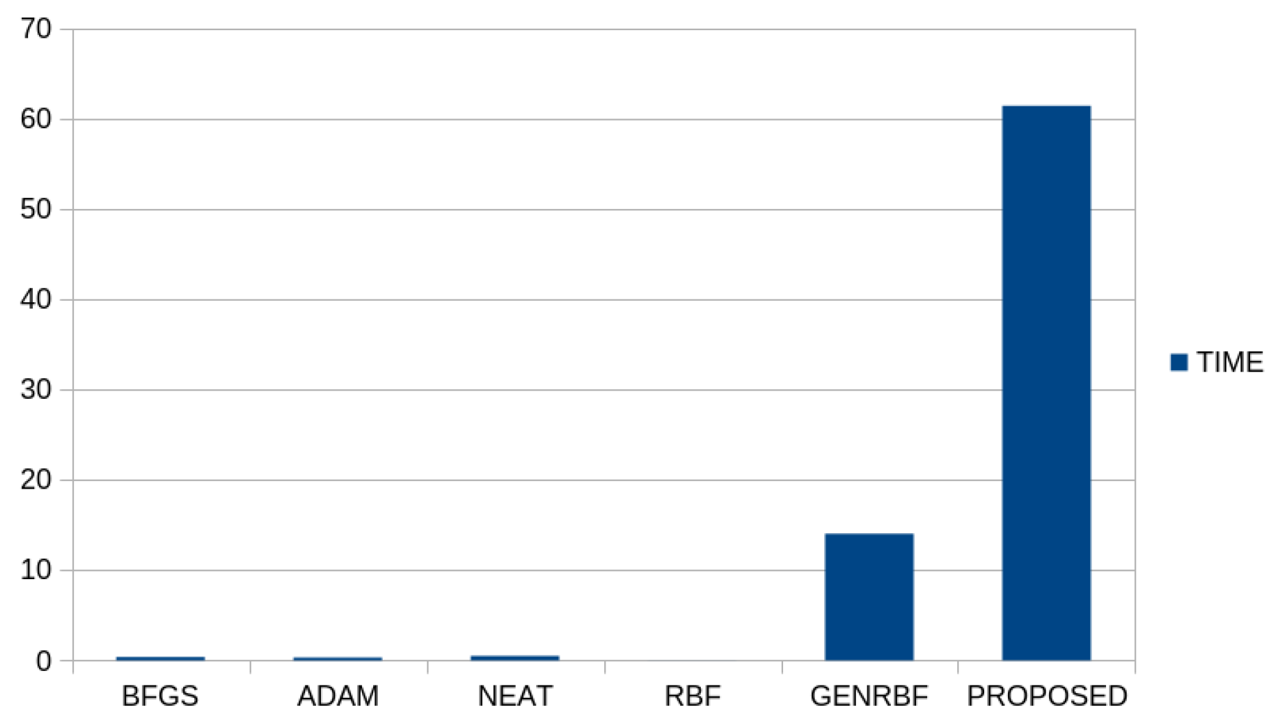
Also, the average execution time for each machine learning technique that was applied to the classification datasets is depicted in Figure 4.

As expected, the proposed technique requires significantly more execution time than all the other techniques in the set, since it consists of the serial execution of global optimization techniques. Moreover, the method entitled GENRBF also required a significant amount of time with respect to other simpler methods in the set. The additional time required by the proposed technique can of course be significantly reduced by the use of parallel processing techniques in its various stages, such as, for example, the use of parallel Simulated Annealing techniques [86]. Moreover, Figure 5 depicts a comparison of the error rates across the models for all classification datasets involved in the conducted experiments.

Table 3 displays the absolute error values resulting from the application of the various machine learning models (BFGS, ADAM, NEAT, RBF-KMEANS, GENRBF, proposed) on the regression datasets. Each row corresponds to a dataset, while each column shows the error of a specific model. The last row records the average error for each model. Lower error values indicate better model performance. The analysis shows that the proposed model has the lowest average error (5.48), making it the most efficient choice among the available models. The second-best model is RBF-KMEANS, with an average error of 9.19, while other models, such as BFGS (26.43) and ADAM (19.62), exhibit significantly higher error values. The performance of the proposed model is particularly impressive on datasets such as BL, where its error is nearly negligible (0.0002), and Mortgage, where it has a very low error (0.14) compared to other models. On datasets like Stock and Plastic, where errors are high across all models, the proposed model still outperforms the other models, with error values of 1.53 and 2.29, respectively. However, there are instances where the performance difference of the proposed model relative to others is small or even unfavorable. For example, on the Laser dataset, the ADAM model has an error of 0.03, slightly higher than the proposed model’s 0.003, while on the HO dataset, the proposed model performs better (0.01), but the RBF-KMEANS model is comparably close (0.03). In summary, the proposed model achieves the lowest average error and the most consistent performance across most datasets, making it an ideal choice for regression problems. Nonetheless, certain models, such as RBF-KMEANS, may demonstrate competitive performance in specific cases, suggesting that model selection depends on the unique characteristics of each dataset.

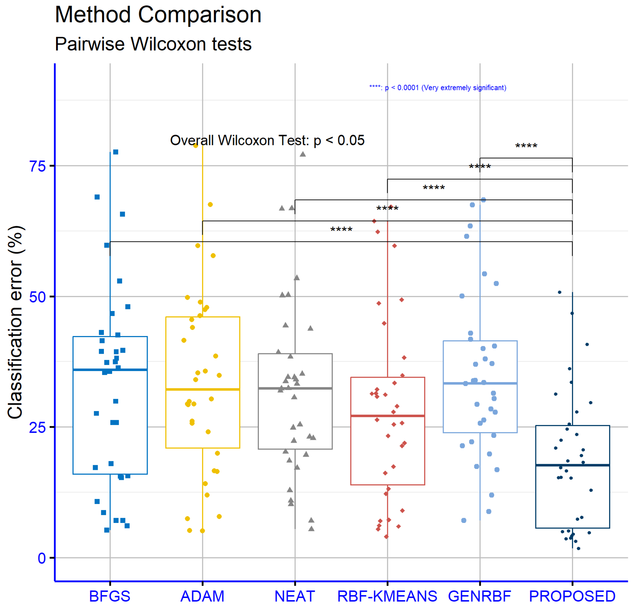
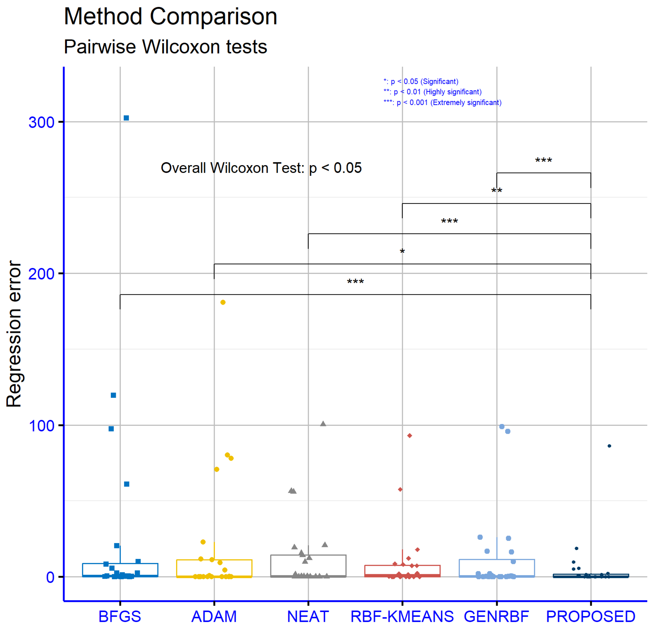
An analysis of significance levels for the classification datasets, as illustrated in Figure 6, reveals that the proposed model statistically significantly outperforms all other models in every comparison pair. Specifically, the p-values indicate strong statistical differences: Proposed vs. BFGS $\left(p={10}^{-8}\right)$, proposed vs. ADAM $\left(p=6.2\times {10}^{-8}\right)$, proposed vs. NEAT $\left(p=2.9\times {10}^{-9}\right)$, proposed vs. RBF-KMEANS $\left(p=1.2\times {10}^{-6}\right)$, and proposed vs. GENRBF $\left(p=1.2\times {10}^{-10}\right)$. These values suggest that the proposed model is significantly better than the others with high reliability.

In Figure 7, which concerns the regression datasets, a similar pattern is observed, though the p-values are generally higher compared to the classification datasets. The proposed model demonstrates statistically significant superiority over the other models in all comparison pairs: Proposed vs. BFGS ($p=0.00011$), proposed vs. ADAM ($p=0.015$), proposed vs. NEAT ($p=0.00016$), proposed vs RBF-KMEANS ($p=0.0016$), and proposed vs. GENRBF ($p=0.00049$). Although the significance is not as strong as in the classification datasets, the proposed model’s superiority remains clear.

3.3. Experiments on the Perturbation Factor a

In order to determine the stability of the proposed technique, another experiment was performed in which the perturbation factor a, presented in the second stage of the proposed technique, took a series of different values.

Table 4. Experimental results for the classification datasets using a series of values for perturbation factor a.

Dataset	$\mathit{a}=0.001$	$\mathit{a}=0.005$	$\mathit{a}=0.01$
Alcohol	31.28%	30.88%	31.77%
Appendicitis	15.27%	15.77%	15.57%
Australian	21.00%	21.03%	20.77%
Balance	12.95%	13.13%	13.29%
Cleveland	50.82%	50.64%	51.11%
Circular	4.19%	4.01%	4.08%
Dermatology	36.13%	36.81%	36.67%
Hayes-Roth	33.54%	33.44%	34.10%
Heart	15.33%	15.15%	15.22%
HeartAttack	18.52%	18.80%	18.88%
HouseVotes	3.74%	3.60%	4.12%
Ionosphere	7.39%	7.38%	7.29%
Liverdisorder	27.92%	28.27%	28.49%
Lymography	20.64%	20.57%	30.33%
Mammographic	17.21%	17.15%	17.14%
Parkinsons	15.35%	14.35%	15.23%
Phoneme	16.62%	16.74%	16.00%
Pima	23.59%	24.09%	23.99%
Popfailures	4.80%	4.82%	4.86%
Regions2	25.54%	25.62%	25.75%
Saheart	29.64%	29.93%	29.22%
Segment	40.83%	41.41%	41.96%
Sonar	18.25%	17.80%	17.83%
Spiral	22.52%	22.00%	22.27%
StatHeart	19.52%	19.35%	19.58%
Student	5.11%	5.03%	5.25%
Transfusion	24.59%	24.70%	24.64%
Wdbc	5.00%	5.05%	5.07%
Wine	7.71%	7.88%	7.90%
Z_F_S	3.16%	3.66%	2.79%
Z_O_N_F_S	46.77%	46.83%	47.06%
ZO_NF_S	3.63%	3.63%	3.63%
ZONF_S	1.79%	1.81%	1.74%
ZOO	4.50%	6.87%	4.60%
Average	18.67%	18.77%	19.06%

presents the error rates of the proposed machine learning model for three different values of the perturbation factor a (0.001, 0.005, 0.01) across various classification datasets. Each row represents a dataset, and the values indicate the model’s error rate for each value of a. The last row includes the average error rate for each value of a. Analysis of the data shows that the smallest value of a (0.001) achieves the lowest average error rate (18.67%), while the largest value (0.01) results in the highest average (19.06%). This suggests that the model generally performs better with smaller values of a, although the difference in averages is minimal. At the dataset level, there are cases where the model’s performance is significantly affected by changes in the parameter. For instance, on the “Lymography” dataset, increasing a from 0.001 to 0.01 leads to a significant increase in the error rate, from 20.64% to 30.33%. A similar trend is observed on the “ZOO” dataset, where the error rate rises from 4.50% to 6.87% for $a=0.005$, but decreases again to 4.60% for $a=0.01$. On the other hand, on datasets like “ZO_NF_S”, the error remains unchanged at 3.63%, regardless of changes in a. Datasets such as “Z_F_S” and “ZONF_S” exhibit nonlinear behavior. On “Z_F_S”, the error rate significantly decreases from 3.16% to 2.79% as a increases from 0.001 to 0.01, while on “ZONF_S”, a similar decrease is observed from 1.79% to 1.74%. In conclusion, the analysis indicates that the perturbation factor a has a notable impact on the performance of the proposed model. Smaller values of a are generally associated with better performance; however, the optimal value may depend on the characteristics of each dataset. Instances where error rates increase or decrease nonlinearly with changes in “a” suggest the need for further investigation into the tuning of “a” for specific applications.

Table 5. Experimental results for regression datasets using different values for parameter a.

Dataset	$\mathit{a}=0.001$	$\mathit{a}=0.005$	$\mathit{a}=0.01$
Abalone	5.10	5.12	5.10
Airfoil	0.004	0.004	0.004
Auto	9.68	9.80	9.89
Baseball	86.19	77.46	81.97
BK	0.153	0.043	0.11
BL	0.0002	0.0002	0.0003
Concrete	0.006	0.006	0.006
Dee	0.16	0.16	0.16
Housing	18.70	18.73	19.20
Friedman	1.45	1.44	1.45
FA	0.019	0.09	0.07
FY	0.077	0.12	0.076
HO	0.01	0.01	0.01
Laser	0.003	0.003	0.003
MB	5.49	0.56	0.48
Mortgage	0.14	0.12	0.13
NT	0.007	0.007	0.007
PL	0.023	0.023	0.023
Plastic	2.29	2.29	2.29
PY	0.019	0.019	0.017
Quake	0.036	0.036	0.036
SN	0.024	0.025	0.024
Stock	1.53	1.52	1.52
Treasury	0.51	0.54	0.47
Average	5.48	4.92	5.13

displays the absolute error values of the proposed machine learning model across various regression datasets for three different values of the perturbation factor a (0.001, 0.005, 0.01). Data analysis reveals that the parameter $a=0.005$ yields the lowest average error (4.92), while the values $a=0.001$ and $a=0.01$ result in slightly higher averages (5.48 and 5.13, respectively). This difference indicates that 0.005 is generally the most suitable value for the model, ensuring better performance in most cases. At the dataset level, the impact of a varies. Some datasets, such as “Airfoil”, “Concrete”, “Dee”, “HO”, “Laser”, “NT”, “PL”, “Plastic”, and “Quake”, show no change in error with variations in a as the error values remain constant. In contrast, other datasets exhibit significant variations. For example, on the “Baseball” dataset, the error decreases from 86.19 for $a=0.001$ to 77.46 for $a=0.005$ then increases again to 81.97 for $a=0.01$. Similarly, on the “MB” dataset, the error drastically decreases from 5.49 for $a=0.001$ to 0.56 for $a=0.005$ and further to 0.48 for $a=0.01$. On datasets like “FA” and “FY”, the error increases as a changes from 0.001 to 0.005, then decreases again for $a=0.01$. On the “Treasury” dataset, the error shows a slight decline as a increases. In conclusion, the parameter a has a significant impact on the model’s performance on certain datasets, while on others, its effect is negligible. The lowest average error observed for $a=0.005$ suggests that this value is generally optimal for the model, though further tuning may be required for specific datasets. Cases with high variability in errors highlight the need for deeper analysis and optimization of the a parameter based on the characteristics of each dataset.

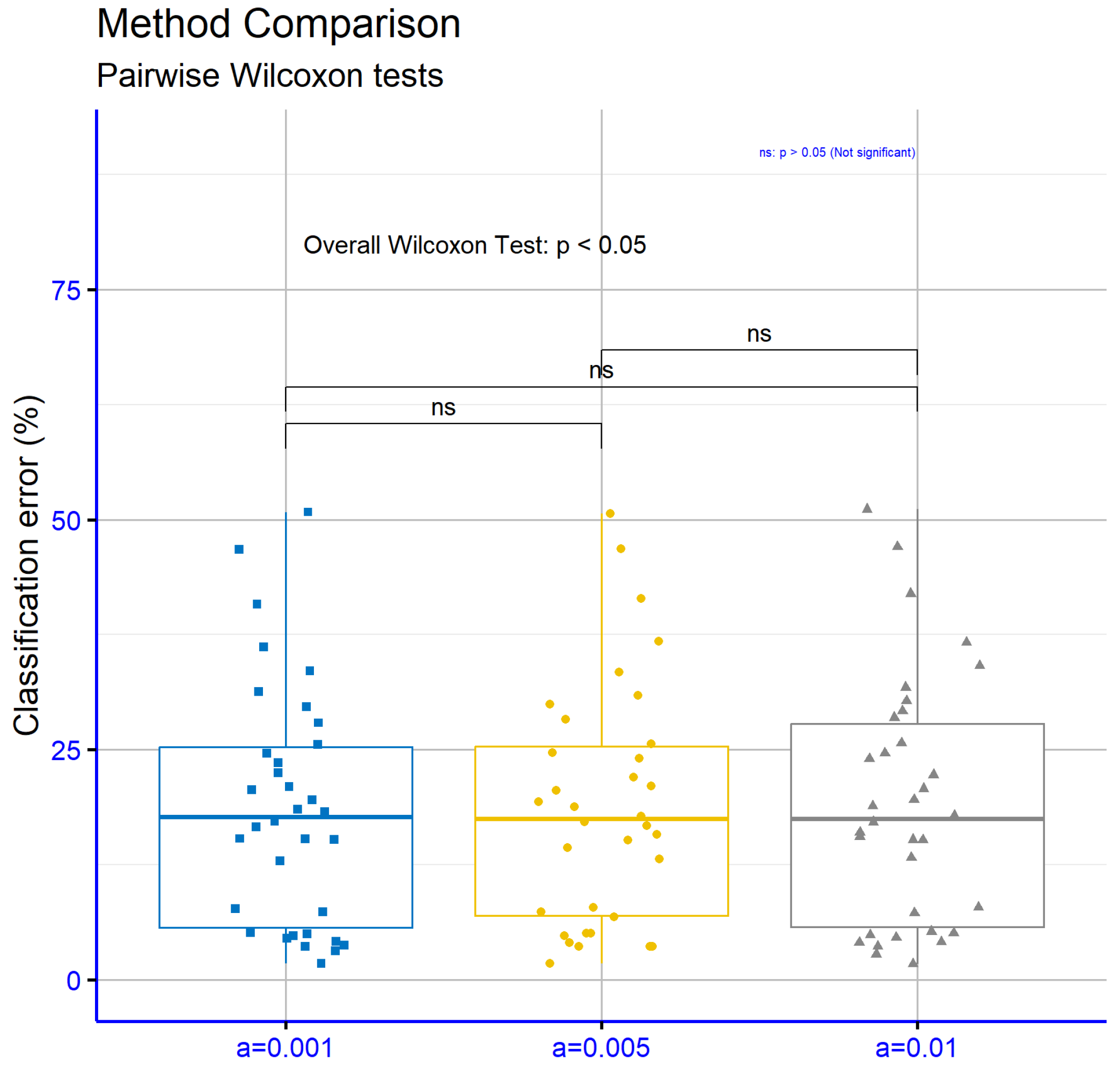
Figure 8 compares different values of the parameter a for the classification datasets. The p-values for the comparisons $a=0.001$ vs. $a=0.005$ ($p=0.36$), $a=0.001$ vs. $a=0.01$ ($p=0.071$), and $a=0.005$ vs. $a=0.01$ ($p=0.17$) indicate that the differences between the parameter values are not statistically significant. This suggests that varying the parameter a within this range does not substantially affect the model’s performance on these datasets.

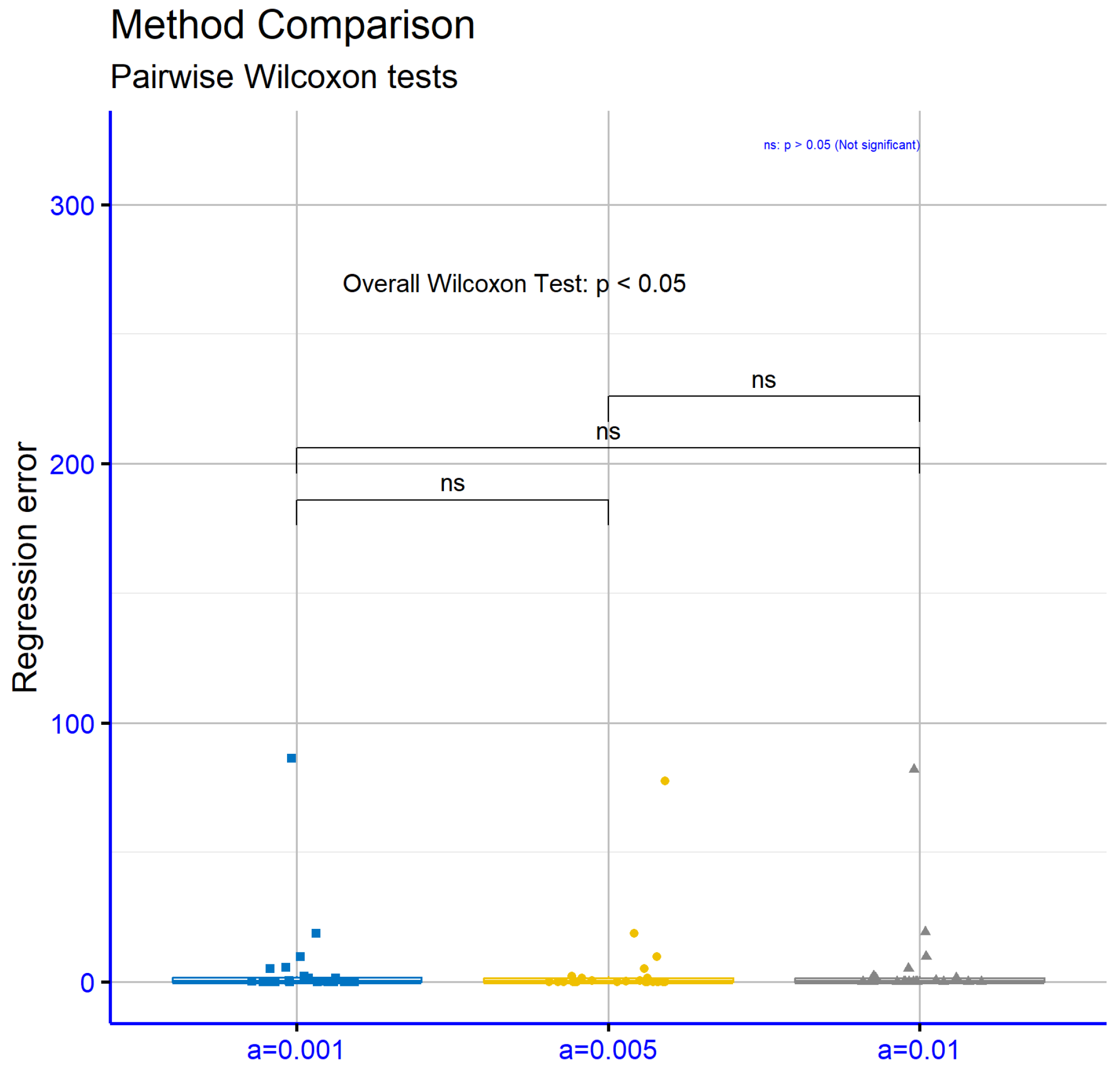
Figure 9 presents corresponding comparisons for the regression datasets, where a similar result is observed. The p-values for the comparisons $a=0.001$ vs. $a=0.005$ ($p=0.75$), $a=0.001$ vs. $a=0.01$ ($p=0.41$), and $a=0.005$ vs. $a=0.01$ ($p=0.94$) indicate the absence of statistically significant differences. This shows that the choice of parameter a does not significantly influence the model’s performance on the regression datasets.

3.4. Experiments on the Parameter F

Another experiment was conducted using the initialization factor F.

Table 6. Experimental results for the classification datasets using a series of values for parameter F.

Dataset	$\mathit{F}=1.5$	$\mathit{F}=3.0$	$\mathit{F}=5.0$	$\mathit{F}=10.0$
Alcohol	25.66%	29.16%	26.14%	31.28%
Appendicitis	16.30%	14.57%	15.50%	15.27%
Australian	23.53%	22.27%	20.81%	21.00%
Balance	15.12%	13.32%	12.68%	12.95%
Cleveland	51.81%	51.41%	50.70%	50.82%
Circular	4.75%	4.15%	4.52%	4.19%
Dermatology	36.69%	36.48%	36.39%	36.13%
Hayes-Roth	46.18%	35.54%	34.18%	33.54%
Heart	16.68%	15.93%	15.68%	15.33%
HeartAttack	27.39%	20.38%	19.03%	18.52%
HouseVotes	3.80%	3.35%	3.85%	3.74%
Ionosphere	12.92%	8.27%	7.41%	7.39%
Liverdisorder	30.48%	29.27%	28.48%	27.92%
Lymography	29.89%	22.41%	21.93%	20.64%
Mammographic	18.00%	17.17%	16.96%	17.21%
Parkinsons	18.25%	17.18%	15.90%	15.35%
Phoneme	17.27%	15.88%	15.90%	16.62%
Pima	24.54%	24.17%	24.05%	23.59%
Popfailures	7.07%	5.35%	5.01%	4.80%
Regions2	26.07%	26.02%	25.78%	25.54%
Saheart	29.75%	28.91%	29.42%	29.64%
Segment	35.81%	36.84%	38.93%	40.83%
Sonar	24.68%	19.25%	16.98%	18.25%
Spiral	13.28%	15.25%	17.88%	22.52%
StatHeart	19.98%	19.58%	19.63%	19.52%
Student	6.14%	6.30%	5.92%	5.11%
Transfusion	25.45%	25.23%	25.19%	24.59%
Wdbc	4.94%	4.92%	4.90%	5.00%
Wine	10.90%	9.37%	8.51%	7.71%
Z_F_S	4.13%	3.73%	3.67%	3.16%
Z_O_N_F_S	46.00%	45.61%	46.57%	46.77%
ZO_NF_S	3.67%	4.19%	3.16%	3.63%
ZONF_S	2.59%	2.37%	2.06%	1.79%
ZOO	11.17%	8.10%	8.00%	4.50%
Average	20.32%	18.88%	18.58%	18.67%

presents the percentage error rates of the proposed machine learning model across various classification datasets for four different values of the parameter F (1.5, 3.0, 5.0, 10.0). Analyzing the data reveals that the parameter F influences the model’s performance, but this effect varies by dataset. The lowest average error rate is observed for $F=5.0$ (18.58%), indicating that this value is generally optimal. For the other values, slightly higher average error rates are noted: 18.88% for $F=3.0$; 18.67% for $F=10.0$; and the highest rate, 20.32%, for $F=1.5$. Examining individual datasets, it is evident that for many of them, increasing F improves performance, as reflected in reduced error rates. Examples include the “Ionosphere”, “Wine”, and “ZONF_S” datasets, where error rates decrease as F increases. On “Ionosphere”, the error rate drops from 12.92% for $F=1.5$ to 7.39% for $F=10.0$. On “Wine”, the error rate decreases from 10.90% for $F=1.5$ to 7.71% for $F=10.0$. Similarly, on “ZONF_S”, the error rate steadily decreases from 2.59% for $F=1.5$ to 1.79% for $F=10.0$. However, there are cases where increasing F does not lead to improvement or results in higher error rates. For example, on the “Segment” dataset, the error rate rises from 35.81% for $F=1.5$ to 40.83% for $F=10.0$. On the “Spiral” dataset, the error rate consistently increases from 13.28% for $F=1.5$ to 22.52% for $F=10.0$. A similar trend is observed on the “Z_O_N_F_S” dataset, where the error rate rises from 46.00% for $F=1.5$ to 46.77% for $F=10.0$. Overall, the parameter F significantly affects the model’s performance, and the optimal value appears to be $F=5.0$, as evidenced by the lowest average error rate. However, the exact impact depends on the characteristics of each dataset, emphasizing the need to fine-tune the parameter value for specific datasets to achieve optimal performance.

Table 7. Experimental results for regression datasets using different values for parameter F.

Dataset	$\mathit{F}=1.5$	$\mathit{F}=3.0$	$\mathit{F}=5.0$	$\mathit{F}=10.0$
Abalone	6.39	5.79	5.57	5.10
Airfoil	0.004	0.004	0.004	0.004
Auto	9.83	9.69	9.67	9.68
Baseball	84.27	83.01	84.57	86.19
BK	0.275	0.048	0.071	0.153
BL	0.41	0.0005	0.0003	0.0002
Concrete	0.006	0.006	0.006	0.006
Dee	0.16	0.16	0.16	0.16
Housing	16.75	17.82	18.07	18.70
Friedman	6.59	3.85	1.67	1.45
FA	0.054	0.03	0.053	0.019
FY	0.216	0.246	0.332	0.077
HO	0.01	0.01	0.01	0.01
Laser	0.022	0.011	0.005	0.003
MB	0.116	0.135	0.307	5.49
Mortgage	0.56	0.59	0.36	0.14
NT	0.007	0.007	0.007	0.007
PL	0.024	0.023	0.023	0.023
Plastic	2.37	2.33	2.31	2.29
PY	2.33	0.049	0.022	0.019
Quake	0.036	0.036	0.036	0.036
SN	0.028	0.04	0.025	0.024
Stock	1.45	1.51	1.49	1.53
Treasury	0.50	0.59	0.43	0.51
Average	5.52	5.25	5.22	5.48

provides the absolute error values of the proposed machine learning model across various regression datasets for four different values of the parameter F (1.5, 3.0, 5.0, 10.0). The data analysis shows that the parameter F affects the model’s performance differently depending on the dataset. The average errors indicate that $F=5.0$ yields the lowest overall error (5.22), followed by $F=3.0$, with an average of 5.25. Higher averages are observed for $F=1.5$ (5.52) and $F=10.0$ (5.48), suggesting that deviating from $F=5.0$ tends to increase error in some cases. Examining the datasets, it is evident that in several cases, increasing F improves performance, reducing error rates. For example, on the “Abalone” dataset, the error decreases from 6.39 for $F=1.5$ to 5.10 for $F=10.0$. Similarly, on the “Friedman” dataset, the error significantly decreases from 6.59 for $F=1.5$ to 1.45 for $F=10.0$. On the “Laser” dataset, the error decreases progressively from 0.022 for $F=1.5$ to 0.003 for $F=10.0$. Conversely, there are datasets where the effect of F is nonlinear or increases the error rate. For instance, on the “Housing” dataset, the error rises from 16.75 for $F=1.5$ to 18.70 for $F=10.0$. On the “MB” dataset, there is a sharp increase in error from 0.116 for $F=1.5$ to 5.49 for $F=10.0$, indicating that F significantly impacts model performance for this dataset. In summary, the parameter F has varying effects on the model’s performance across different datasets. While the average indicates that $F=5.0$ is the optimal choice, precise optimization of the parameter should be dataset-specific. Additionally, extreme parameter values may lead to significant performance degradation in certain datasets, as seen in examples like “MB” and “Housing”.

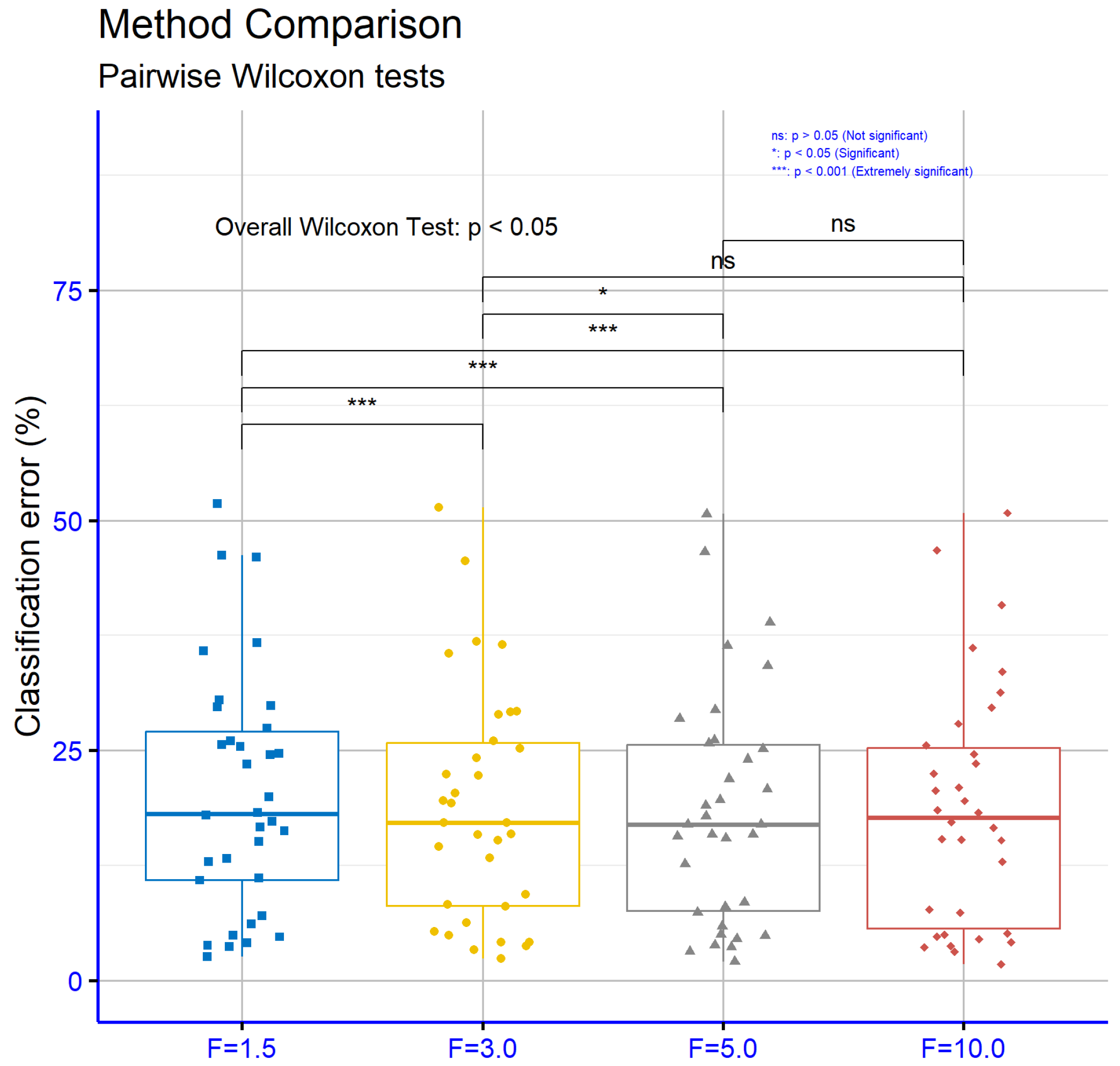
In Figure 10, which compares different values of the parameter F for the classification datasets, several statistically significant differences are observed. The p-values for the comparisons $F=1.5$ vs. $F=3.0$ ($p=0.00019$), $F=1.5$ vs. $F=5.0$ ($p=0.00012$), and $F=1.5$ vs. $F=10.0$ ($p=0.00069$) indicate a strong difference in the model’s performance. In contrast, the values for the comparisons $F=3.0$ vs. $F=5.0$ ($p=0.027$), $F=3.0$ vs. $F=10.0$ ($p=0.062$), and $F=5.0$ vs. $F=10.0$ ($p=0.23$) show that the differences between larger values of the parameter F are less significant.

Figure 11 examines comparisons of the parameter F for the regression datasets and shows no statistically significant differences. The p-values for the comparisons $F=1.5$ vs. $F=3.0$ ($p=0.18$), $F=1.5$ vs. $F=5.0$ ($p=0.15$), $F=1.5$ vs. $F=10.0$ ($p=0.21$), $F=3.0$ vs. $F=5.0$ ($p=0.7$), $F=3.0$ vs. $F=10.0$ ($p=0.54$), and $F=5.0$ vs. $F=10.0$ ($p=0.89$) indicate that variations in the value of the parameter F do not significantly affect the model’s performance on the regression datasets. This may suggest greater stability of the model to changes in this parameter compared to the classification datasets.

3.5. Experiments on Number of Generations

In order to evaluate the convergence of the genetic algorithm, an additional experiment was conducted where the number of generations was altered from 25 to 200. The experimental results using the proposed method for the classification datasets are depicted in

Table 8. Experimental results using the proposed method and a series of numbers of generations for the classification datasets.

Dataset	${\mathit{N}}_{\mathit{g}}=25$	${\mathit{N}}_{\mathit{g}}=50$	${\mathit{N}}_{\mathit{g}}=100$	${\mathit{N}}_{\mathit{g}}=200$
Alcohol	38.19%	34.98%	32.45%	31.28%
Appendicitis	15.53%	15.40%	16.00%	15.27%
Australian	23.92%	23.77%	22.56%	21.00%
Balance	19.08%	16.71%	13.57%	12.95%
Cleveland	51.08%	50.85%	51.26%	50.82%
Circular	4.76%	4.94%	5.13%	4.19%
Dermatology	36.12%	36.17%	35.81%	36.13%
Hayes-Roth	37.85%	35.56%	33.56%	33.54%
Heart	15.58%	15.62%	15.52%	15.33%
HeartAttack	20.28%	19.14%	18.89%	18.52%
HouseVotes	3.46%	3.81%	3.78%	3.74%
Ionosphere	9.16%	8.23%	7.95%	7.39%
Liverdisorder	27.77%	28.23%	28.26%	27.92%
Lymography	19.62%	20.26%	20.62%	20.64%
Mammographic	16.99%	16.90%	16.92%	17.21%
Parkinsons	14.58%	14.51%	13.76%	15.35%
Phoneme	17.29%	17.45%	17.21%	16.62%
Pima	23.83%	24.09%	23.87%	23.59%
Popfailures	4.93%	4.61%	4.70%	4.80%
Regions2	25.65%	25.74%	25.60%	25.54%
Saheart	28.50%	29.23%	29.07%	29.64%
Segment	41.81%	42.77%	43.65%	40.83%
Sonar	21.77%	20.45%	19.60%	18.25%
Spiral	31.82%	28.09%	26.07%	22.52%
StatHeart	20.05%	20.09%	19.93%	19.52%
Student	4.43%	4.62%	5.21%	5.11%
Transfusion	24.82%	24.72%	24.39%	24.59%
Wdbc	4.97%	5.10%	5.25%	5.00%
Wine	7.80%	7.37%	7.69%	7.71%
Z_F_S	3.52%	3.55%	3.59%	3.16%
Z_O_N_F_S	49.56%	48.04%	47.77%	46.77%
ZO_NF_S	4.19%	3.97%	3.77%	3.63%
ZONF_S	2.22%	1.92%	2.00%	1.79%
ZOO	8.57%	8.40%	7.60%	4.50%
Average	19.99%	19.57%	19.21%	18.67%

and for the regression datasets in

Table 9. Experimental results using the proposed method and a series of numbers of generations for the regression datasets.

Dataset	${\mathit{N}}_{\mathit{g}}=25$	${\mathit{N}}_{\mathit{g}}=50$	${\mathit{N}}_{\mathit{g}}=100$	${\mathit{N}}_{\mathit{g}}=200$
Abalone	6.08	5.74	5.65	5.10
Airfoil	0.004	0.004	0.004	0.004
Auto	10.37	9.71	9.60	9.68
Baseball	89.23	90.91	81.42	86.19
BK	0.028	0.032	0.10	0.153
BL	0.001	0.0003	0.0006	0.0002
Concrete	0.007	0.007	0.006	0.006
Dee	0.16	0.16	0.17	0.16
Housing	17.72	18.00	18.23	18.70
Friedman	3.22	2.41	1.81	1.45
FA	0.025	0.051	0.05	0.019
FY	0.078	0.29	0.17	0.077
HO	0.009	0.009	0.009	0.01
Laser	0.004	0.003	0.003	0.003
MB	0.15	0.37	0.27	5.49
Mortgage	0.29	0.23	0.48	0.14
NT	0.006	0.006	0.007	0.007
PL	0.02	0.018	0.016	0.023
Plastic	2.33	2.32	2.22	2.29
PY	0.02	0.018	0.016	0.019
Quake	0.036	0.036	0.036	0.036
SN	0.026	0.025	0.025	0.024
Stock	2.29	1.96	1.98	1.53
Treasury	0.82	0.75	0.75	0.51
Average	5.54	5.55	5.13	5.48

.

In Table 8, the experimental results indicate a general trend of decreasing error rates as the number of generations $N_g$ increases from 25 to 200. This reduction suggests that increasing $N_g$ improves the performance of the genetic algorithm, as it allows the model to better approximate the optimal solution. For most datasets, the lowest error rate is observed when $N_g=200$. For instance, on the “Alcohol” dataset, the error rate decreased from 38.19% to 31.28%, while a significant reduction was also observed in the “Sonar” dataset, from 21.77% to 18.25%. Similar reductions were noted on several other datasets, such as “Spiral” (31.82% to 22.52%) and “ZO_NF_S” (4.19% to 3.63%). However, there are datasets like “Mammographic” and “Lymography” where the changes are minor and not consistently positive, indicating that increasing the number of generations does not always have a dramatic impact on performance. The overall average error rate across all datasets steadily decreases, from 19.99% when $N_g=25$ to 18.67% when $N_g=200$. This confirms the general trend of the genetic algorithm converging towards improved solutions with more generations. The statistical analysis of the results demonstrates that increasing the number of generations is effective in the majority of cases, enhancing the accuracy of the proposed method on classification datasets. Nonetheless, the performance improvement appears to also depend on the specific characteristics of each dataset as well as the inherent properties of the method.

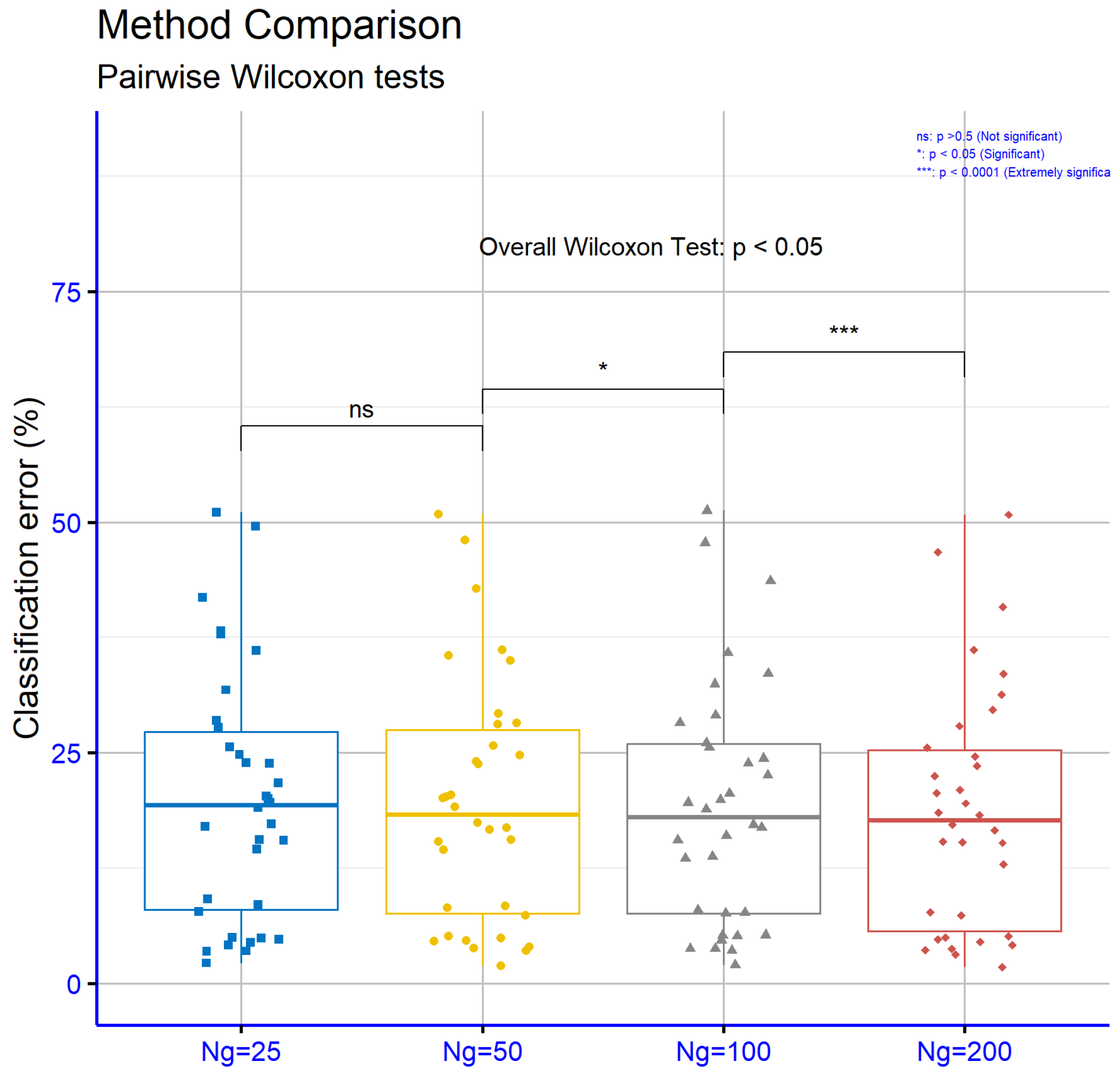
Figure 12 presents the significance levels p for the experiments conducted on the classification datasets with various models. The results indicate that the difference between $N_g=25$ and $N_g=50$ is not statistically significant, as p is 0.12. In contrast, the transition from $N_g=50$ to $N_g=100$ is marginally significant, with p = 0.048, suggesting that the increase in generations begins to influence model performance. Finally, the difference between $N_g=100$ and $N_g=200$ shows high statistical significance, with p = 0.00083, confirming that the increase in the number of generations significantly contributes to performance improvement.

In Table 9, the experimental findings suggest that the convergence behavior of the genetic algorithm on regression datasets shows varied patterns as the number of generations $N_g$ increases from 25 to 200. Specifically, a reduction in error values is observed on several datasets, while on others, errors either increase or remain stable. For instance, on the “Abalone” dataset, the error decreases steadily from 6.08 at $N_g=25$ to 5.10 at $N_g=200$, indicating improved performance. On the “Friedman” dataset, there is a significant reduction from 3.22 to 1.45, demonstrating a clear trend of convergence toward optimal solutions. Similar reductions are observed on “Stock” (2.29 to 1.53) and “Treasury” (0.82 to 0.51). However, there are datasets such as “Auto”, where the reduction is negligible, and the error slightly increases from 9.60 at $N_g=100$ to 9.68 at $N_g=200$. Furthermore, on the “Housing” dataset, a gradual increase in error is observed, from 17.72 to 18.70, suggesting that the increased number of generations did not improve performance. On the “MB” dataset, the error rises significantly, from 0.15 at $N_g$ = 25 to 5.49 at $N_g=200$, indicating potential instability of the method on this specific dataset. The average across all datasets shows a nonlinear pattern, with values fluctuating. The average error decreases from 5.54 at $N_g$ = 25 to 5.13 at $N_g=100$, but then increases to 5.48 at $N-=200$. This indicates that increasing the number of generations does not always lead to consistent improvement in performance across regression datasets. In conclusion, the statistical analysis reveals that increasing the number of generations $N_g$ can improve the performance of the genetic algorithm on certain datasets; however, its impact is not always consistent. The outcome depends on the specific characteristics of each dataset as well as the inherent properties of the method.

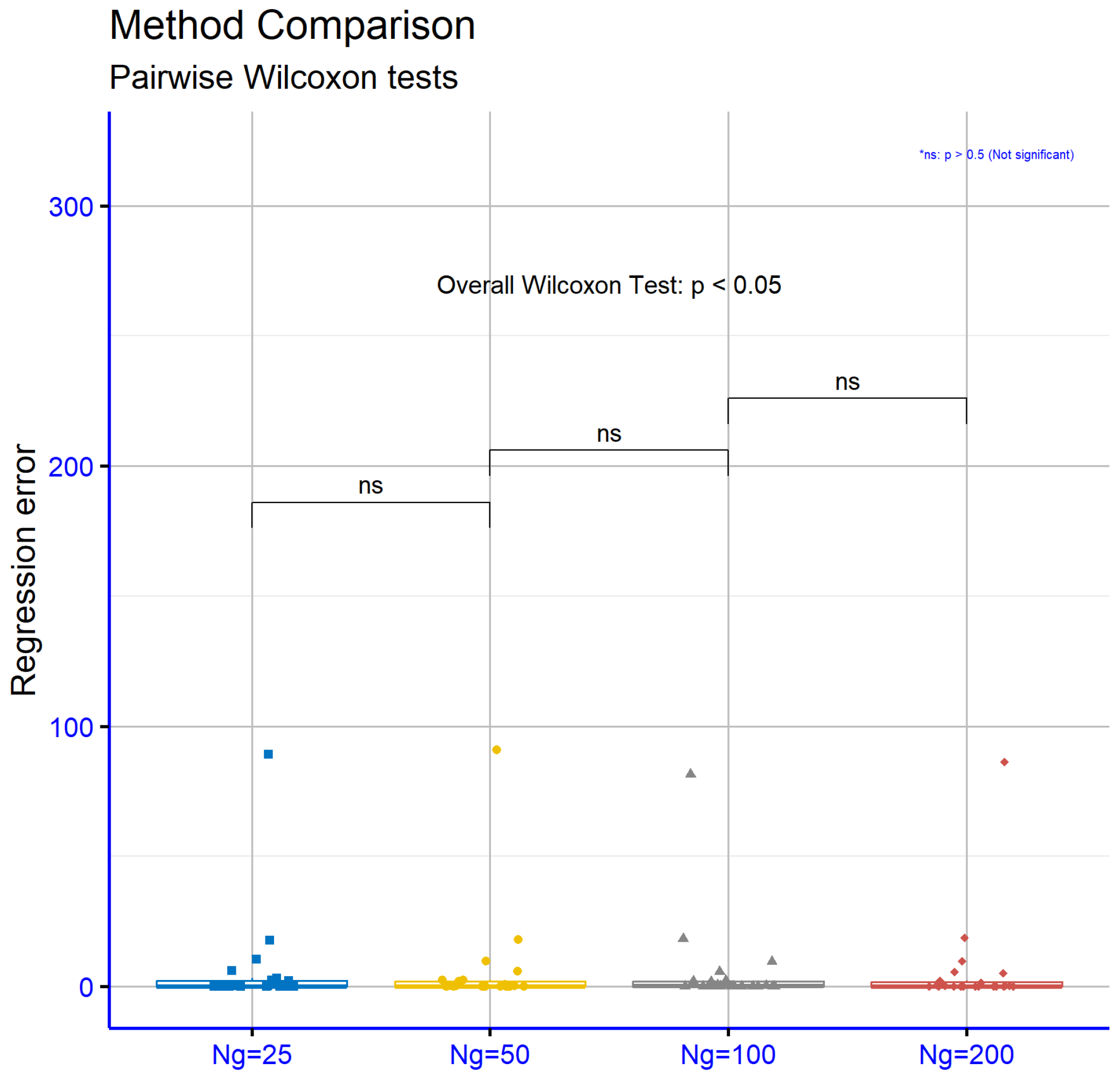
Figure 13 pertains to the regression datasets and shows that the performance differences between consecutive $N_g$ values are not statistically significant. Specifically, for $N_g=25$ versus $N_g=50$, p is 0.46, for $N_g=50$ versus $N_g=100$, p is 0.27, and for $N_g=100$ versus $N_g=200$, p is 0.9. These results suggest that increasing the number of generations in regression datasets does not lead to significant performance changes, indicating that the characteristics of these datasets may limit the effectiveness of the approach.

4. Conclusions

The article focuses on optimizing the parameter tuning process in radial basis function networks through a multidimensional and innovative approach that combines techniques such as Simulated Annealing and genetic algorithms. The proposed method surpasses traditional two-stage approaches, where parameters are typically determined using fixed processes like K-means clustering followed by a split between training and validation phases. Instead, the article introduces a three-phase process. In the first phase, initial parameter estimation is performed using K-means, ensuring a stable starting point. In the second phase, the application of Simulated Annealing provides an advanced mechanism for exploring the parameter space, avoiding local minima and examining a broader range of potential values. Finally, the third phase integrates genetic algorithms, enabling the optimization of parameters based on the model’s actual performance. This process ensures a comprehensive and adaptive approach, reducing the likelihood of overfitting and numerical instability. The novelty of the method lies not only in the three-phase process but also in the model’s ability to adapt to datasets with diverse characteristics, such as those involving complex nonlinear relationships or multidimensional dependencies. The experimental results demonstrate the method’s superiority compared to traditional techniques, such as BFGS, ADAM, NEAT, and RBF-KMEANS, achieving improvements in terms of average error rates across both classification and regression datasets.

The article’s conclusions clearly highlight the superiority of the proposed method. In classification datasets, the method achieves lower average error rates, particularly when the parameters a and F are optimally configured. For instance, in classification datasets, the parameter F significantly influences performance, with $F=5.0$ proving to be the most effective value in many cases. On datasets such as “Ionosphere” and “Wine”, dramatic reductions in error rates are observed as the value of F increases, emphasizing the importance of selecting this parameter correctly. Similarly, on the regression datasets, the proposed model demonstrates exceptional performance, with notable examples including datasets like “Abalone” and “Friedman”, where the error decreases significantly compared to traditional techniques. The “MB” dataset is particularly interesting, as the use of Simulated Annealing contributes to a substantial performance improvement, avoiding errors commonly encountered in traditional approaches. Despite the generally positive results, there are cases where the method’s performance is suboptimal, such as on the “Segment” dataset, indicating that the method is not universally generalizable without adjustment to the characteristics of each dataset. The need for further research on the parameters a and F is evident, as these parameters critically impact performance across numerous datasets.

For the future, the article proposes numerous directions for further exploration and development. Initially, applying the method to more diverse data categories, such as time series, image data, or even genetic data, could broaden its application scope. Additionally, the dynamic adjustment of the parameters a and F during training, using reinforcement learning techniques, could further enhance performance by eliminating the need for manual tuning. Furthermore, integrating the method into deep learning systems, such as convolutional or recurrent neural networks, could lead to hybrid approaches that combine the flexibility of RBFs with the computational power of deep neural networks. Moreover, investigating the robustness of the method in environments with dynamic or imbalanced data could provide additional insights into its generalizability. Finally, analyzing the method’s performance on big data and integrating it with technologies like distributed processing or cloud computing could open new avenues, enabling its scalability to larger-scale problems. The methodology proposed in the article not only sets new standards for the performance of RBFs but also paves the way for further innovation in the field of machine learning.