Article

Hybrid Optimization Algorithm for Solving Attack-Response Optimization and Engineering Design Problems

1
King Abdullah the II IT School, Department of Computer Science, The University of Jordan, Amman 11942, Jordan
2
Data Science and Artificial Intelligence Department, Faculty of Information Technology, University of Petra, Amman 11196, Jordan
3
Computer Science Department, Faculty of Information Technology, University of Petra, Amman 11196, Jordan
*
Author to whom correspondence should be addressed.
Algorithms 2025, 18(3), 160; https://doi.org/10.3390/a18030160
Submission received: 24 January 2025 / Revised: 8 February 2025 / Accepted: 5 March 2025 / Published: 10 March 2025
(This article belongs to the Section Algorithms for Multidisciplinary Applications)

Abstract

:
This paper presents JADEDO, a hybrid optimization method that merges the dandelion optimizer’s (DO) dispersal-inspired stages with JADE’s (adaptive differential evolution) dynamic mutation and crossover operators. By integrating these complementary mechanisms, JADEDO effectively balances global exploration and local exploitation for both unimodal and multimodal search spaces. Extensive benchmarking against classical and cutting-edge metaheuristics on the IEEE CEC2022 functions—encompassing unimodal, multimodal, and hybrid landscapes—demonstrates that JADEDO achieves highly competitive results in terms of solution accuracy, convergence speed, and robustness. Statistical analysis using Wilcoxon sum-rank tests further underscores JADEDO’s consistent advantage over several established optimizers, reflecting its proficiency in navigating complex, high-dimensional problems. To validate its real-world applicability, JADEDO was also evaluated on three engineering design problems (pressure vessel, spring, and speed reducer). Notably, it achieved top-tier or near-optimal designs in constrained, high-stakes environments. Moreover, to demonstrate suitability for security-oriented tasks, JADEDO was applied to an attack-response optimization scenario, efficiently identifying cost-effective, low-risk countermeasures under stringent time constraints. These collective findings highlight JADEDO as a robust, flexible, and high-performing framework capable of tackling both benchmark-oriented and practical optimization challenges.

1. Introduction

The rapid advancement of engineering and technological fields has significantly transformed the landscape of design and problem-solving. As industries push the boundaries of innovation, they face increasingly intricate and multifaceted design problems that demand not only creativity but also rigorous analytical methods [1]. Traditional optimization techniques often fall short in addressing these complex challenges due to the inherent nature of modern design problems. These problems are frequently characterized by high dimensionality, where the number of variables or parameters involved is vast, leading to a highly intricate solution space [2]. Additionally, the non-linearity of these problems means that the relationships between variables are not straightforward or proportional, further complicating the optimization process. Moreover, multiple constraints, such as resource limitations, regulatory requirements, and environmental considerations, add layers of complexity to the problem [3].
To effectively tackle such challenges, there is a growing need for advanced optimization algorithms that can navigate these complexities with precision and efficiency. This is where hybrid optimization methods come into play. These methods represent a sophisticated approach that merges the strengths of various algorithms, each contributing its unique capabilities to the overall process [4]. For instance, hybrid methods may combine global optimization techniques, which are adept at exploring large and complex solution spaces, with local optimization techniques, which excel at fine-tuning solutions within a specific region of the search space. By integrating these approaches, hybrid optimization methods can offer a more balanced and robust solution strategy, addressing both the broad exploration of potential solutions and the detailed refinement of those solutions [5].
The power of hybrid optimization lies in its ability to enhance both performance and reliability. Performance is improved by combining different algorithms that can adapt to various aspects of the problem and avoid common pitfalls, such as becoming trapped in local optima [6]. Reliability is achieved by leveraging the complementary strengths of the algorithms, leading to more consistent and dependable results. This holistic approach not only improves the efficiency of finding optimal solutions but also ensures that the solutions are more applicable and practical in real-world scenarios. As engineering and technological fields continue to evolve, the role of hybrid optimization methods becomes increasingly crucial in addressing the sophisticated and dynamic nature of modern design problems [7].
In this paper, we introduce a hybrid optimization framework called JADEDO, designed to address both benchmark-driven and practical optimization challenges. JADEDO combines the strengths of two established metaheuristics, namely, (1) dandelion optimizer (DO): Inspired by the dispersal of dandelion seeds, DO employs a sequence of stages (dispersal, propagation, and competition) that collectively push the search process toward promising regions while maintaining the potential to escape local optima. (2) Adaptive differential evolution (JADE): Known for its adaptive mutation strategies and crossover operators, JADE dynamically adjusts parameter settings (e.g., mutation factor and crossover rate) to balance exploration and exploitation over the course of the search.
By merging these two paradigms, JADEDO leverages DO’s robust dispersal mechanisms to broaden global exploration, while JADE’s adaptive operators refine local searches effectively. The resultant synergy endows JADEDO with heightened flexibility and robustness across different problem landscapes—unimodal, multimodal, and hybrid.
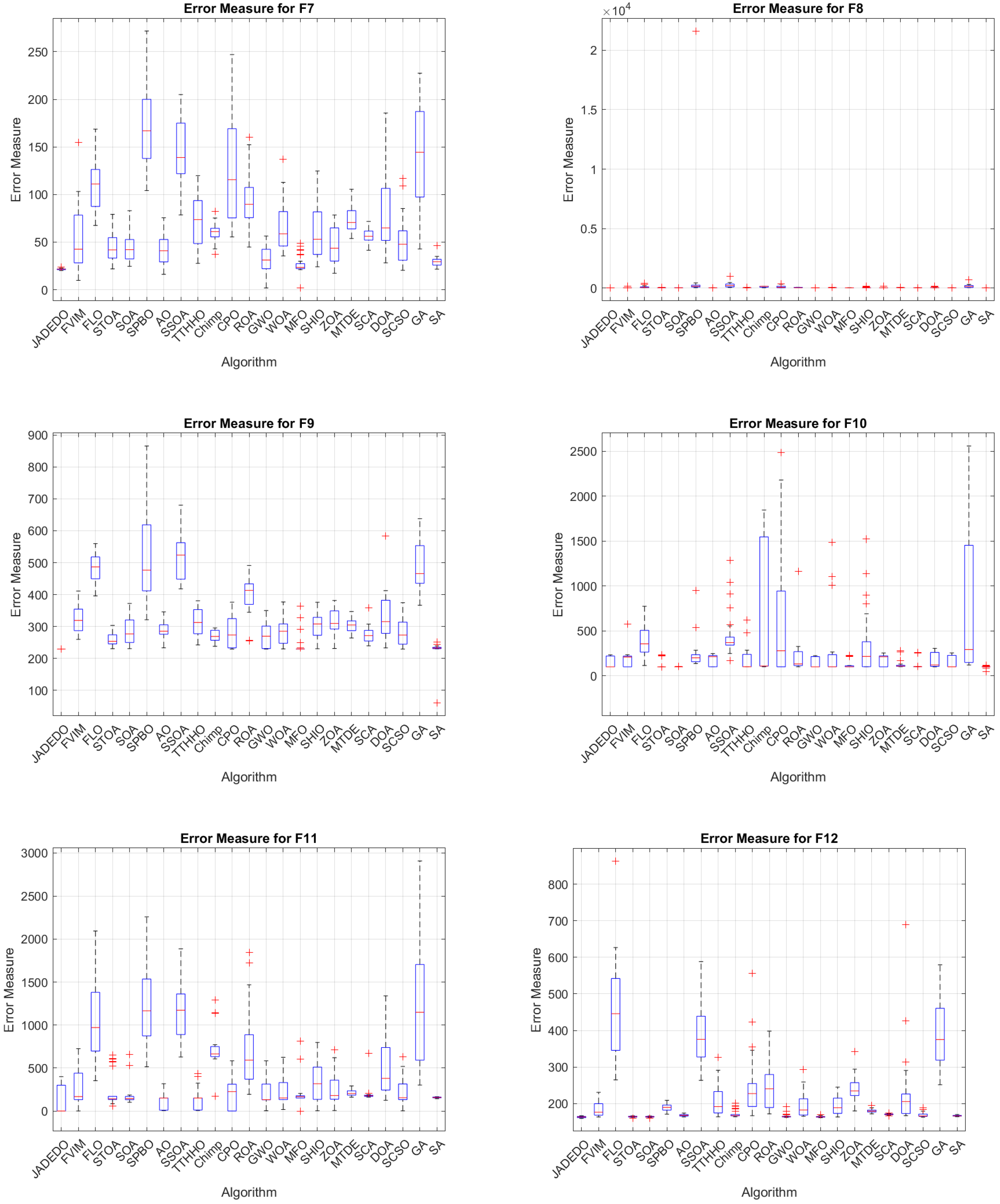
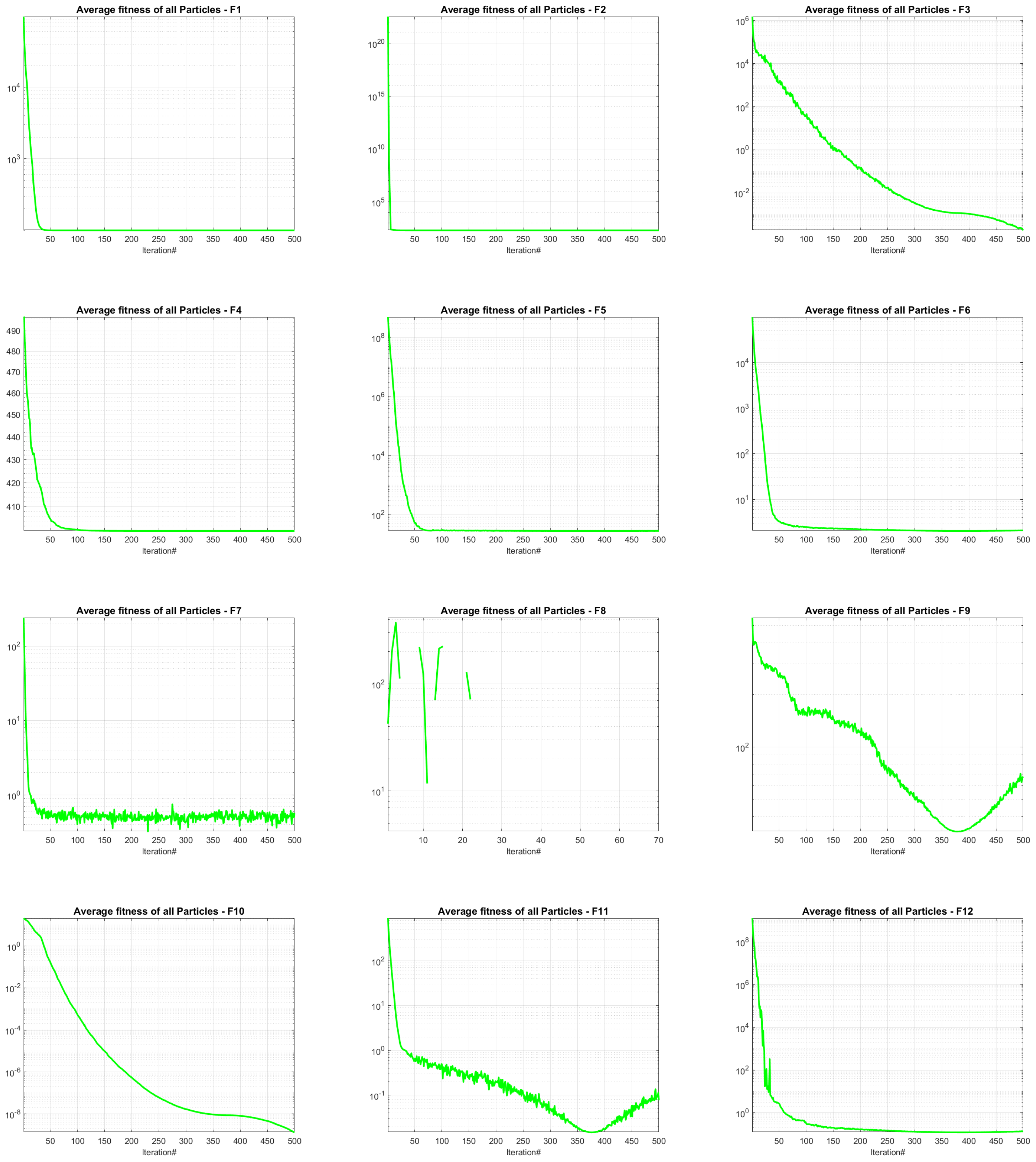
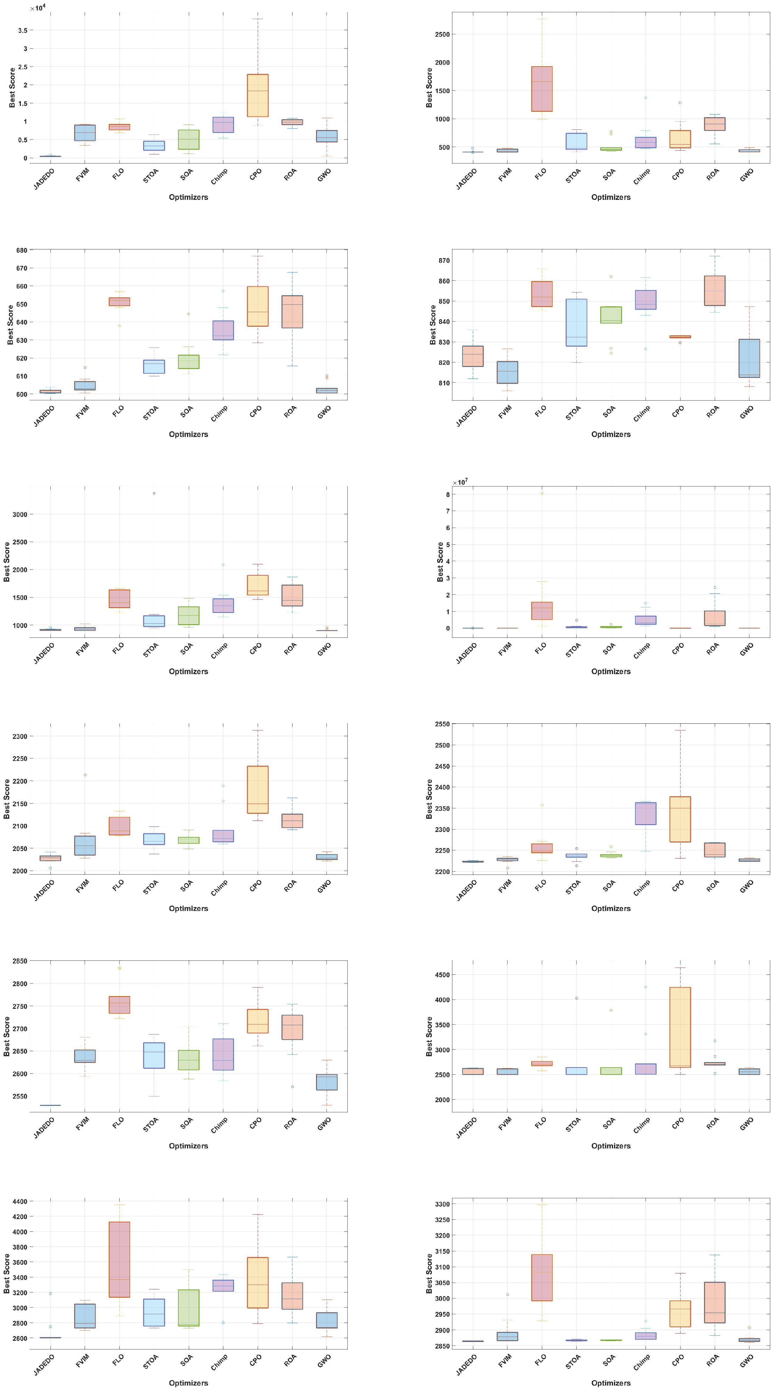
To validate its performance, JADEDO is extensively benchmarked against a suite of well-known and cutting-edge metaheuristics using the IEEE CEC2022 test functions. These functions impose diverse optimization challenges, ranging from simple unimodal functions that test convergence speed to intricate multimodal and hybrid landscapes that stress exploration capabilities. The experiments highlight that JADEDO achieves competitive or superior results in terms of both solution quality (precision) and convergence speed. Statistical significance, assessed via the Wilcoxon sum-rank test, underscores JADEDO’s consistent advantage over several established optimizers.
Beyond synthetic benchmarks, we demonstrate the practical value of JADEDO in two domains. First, we address three engineering design problems with high stakes and multiple constraints: the pressure vessel, the spring, and the speed reducer. In each case, JADEDO attained highly competitive designs, underscoring its potential to reduce costs, maintain reliability, and meet strict physical constraints. Second, we apply JADEDO to an attack-response optimization problem, where timely and cost-effective countermeasures against potential threats must be identified. JADEDO excels in this domain by swiftly converging on strategies that minimize both risk and resource expenditure.

Key Contributions

  • Proposal of a novel hybrid method: We introduce JADEDO, a new optimization algorithm that fuses the dispersal stages of the dandelion optimizer with the adaptive mutation and crossover mechanisms of JADE, aiming to leverage both global exploration and local exploitation in a unified framework.
  • Benchmark validation: Comprehensive experiments on the IEEE CEC2022 benchmark functions, encompassing unimodal, multimodal, and hybrid landscapes, demonstrate JADEDO’s superior or highly competitive performance in terms of solution accuracy, convergence speed, and robustness.
  • Real-world applicability: We validate JADEDO on three engineering design problems (pressure vessel, spring, and speed reducer) and an attack-response optimization scenario. In each case, JADEDO identifies effective solutions under strict constraints, highlighting its capacity to handle high-stakes, complex optimization tasks.

2. Literature Review

Recent advancements in optimization techniques have increasingly focused on hybrid algorithms to solve complex engineering design problems, capitalizing on the strengths of multiple approaches to enhance solution quality and convergence speed. Verma and Parouha [8] introduced an advanced hybrid algorithm, haDEPSO, which integrates differential evolution (aDE) with particle swarm optimization (aPSO). The aDE component prevents premature convergence through novel mutation, crossover, and selection strategies, while aPSO utilizes gradually varying parameters to avoid stagnation. This hybrid approach was validated on five engineering design problems, demonstrating superior convergence characteristics through extensive numerical, statistical, and graphical analyses.
Panagant et al. [9] introduced HMPANM, a hybrid optimization algorithm combining Marine Predators Optimization with the Nelder–Mead method to improve local exploitation capabilities. This algorithm was applied to the structural design optimization of automotive components, proving its effectiveness in achieving optimal designs under competitive industrial conditions. Yildiz and Mehta [10] further explored hybrid metaheuristics for automotive engineering design, applying the hybrid Taguchi Salp Swarm–Nelder–Mead algorithm (HTSSA-NM) and manta ray foraging optimization (MRFO) to optimize the structure of automobile brake pedals. The results showed HTSSA-NM’s superiority in minimizing mass while achieving better shape optimization compared to other algorithms.
Duan and Yu [11] introduced a collaboration-based hybrid grey wolf optimizer and sine cosine algorithm (cHGWOSCA), which enhances global exploration through SCA while maintaining a balance with exploitation via a weight-based position update mechanism. This algorithm demonstrated high performance on IEEE CEC benchmarks and real-world engineering problems. Similarly, Barshandeh et al. [12] proposed the hybrid multi-population algorithm (HMPA), combining artificial ecosystem-based optimization (AEO) with Harris Hawks optimization (HHO). HMPA employs strategies like a Lévy flight, local search mechanisms, and quasi-oppositional learning, resulting in improved exploration and exploitation.
Su et al. [13] introduced the hybrid political algorithm (HPA), which enhances the political optimizer’s exploration process for global optima by improving particle movement during computation. HPA was tested on engineering optimization problems, outperforming other algorithms in avoiding local optima. Uray et al. [14] presented a Taguchi method-integrated hybrid harmony search algorithm (HHS), focusing on parameter optimization through statistical estimation of control parameter values, achieving rapid convergence in engineering design problems.
Fakhouri et al. [15] introduced PSOSCANMS, a hybrid algorithm that integrates PSO with the sine cosine algorithm (SCA) and the Nelder–Mead simplex (NMS) technique. This approach addresses PSO’s drawbacks, such as low convergence rates and local minima entrapment, by enhancing exploration–exploitation balance through mathematical formulations from SCA and NMS. The algorithm was benchmarked on various optimization problems, demonstrating significant improvements over traditional PSO.
Kumar et al. [16] introduced a hybrid algorithm that integrates quantum-behaved particle swarm optimization (QPSO) with a binary tournament technique to tackle bound-constrained optimization problems. This algorithm demonstrated superior performance on several benchmark problems and engineering design challenges, offering promising results. Hu et al. [17] developed the hybrid CSOAOA algorithm, combining the arithmetic optimization algorithm (AOA) with point set, optimal neighborhood learning, and crisscross strategies. CSOAOA was highly effective, with improved precision, faster convergence rates, and better solution quality.
Bose [18] conducted an experimental study on hybrid composite materials using laser engineering net shaping (LENS) and applied optimization techniques like desirable gray relational analysis (DGRA) to improve material properties. The optimized parameters led to significant improvements in cooling rate and hardness, contributing to material engineering advancements. Wang [19] explored genetic hybrid optimization for multi-objective engineering project management, showcasing the advantages of hybrid optimization in handling complex, multi-objective tasks.
Li and Ma [20] proposed a hybrid algorithm, CWDEPSO, integrating differential evolution concepts into PSO to prevent premature convergence and enhance local search. Pham et al. [21] introduced nSCA, an enhancement to the sine cosine algorithm, by incorporating roulette wheel selection and opposition-based learning. nSCA outperformed leading-edge methods like genetic algorithms and PSO across various optimization problems, making it a strong candidate for complex engineering challenges.

2.1. Overview of Adaptive Differential Evolution with an Optional External Archive (JADE)

Adaptive differential evolution with an optional external archive, usually referred to as JADE, is an improved variant of differential evolution (DE). Its design focuses on increasing convergence speed and maintaining solution diversity. JADE accomplishes these goals by adapting two central parameters—the scale factor and crossover probability—and by keeping an external archive of solutions. This archive retains historical information that can help the algorithm explore the search space more effectively.
JADE employs a special mutation strategy referred to as current-to-pbest. Equation (24) shows how the mutant vector v i , G is formed from the target vector x i , G at generation G.
v i , G = x i , G + F i x pbest , G x i , G + F i x r 1 , G x r 2 , G
In Equation (24), v i , G is the mutant vector, x i , G is the current (target) vector, and F i is the scale factor for the ith individual. The vector x pbest , G is randomly selected from the top p × 100 % best solutions in the current population. The parameter p is a small positive constant (for instance, 0.05 ) controlling how many top solutions can be chosen as x pbest , G . The vectors x r 1 , G and x r 2 , G are selected randomly from the population and from the union of the population and an external archive, respectively. This archive, denoted by A , stores older solutions that were replaced in previous generations.
After producing the mutant vector, JADE relies on binomial crossover to generate a trial vector u i , G by mixing the components of v i , G and x i , G . The crossover step is illustrated in Equation (16).
u i , G d = v i , G d , if rand d C R i or d = rand _ index , x i , G d , otherwise ,
In Equation (16), u i , G d is the dth component of the trial vector u i , G . The term v i , G d represents the dth component of the mutant vector v i , G , while x i , G d is the dth component of the target vector x i , G . The quantity C R i is the crossover probability for the ith individual, and rand d is a uniformly distributed random number in [ 0 , 1 ] . The index rand _ index ensures that at least one component of u i , G is inherited from the mutant vector.
The selection step compares u i , G against x i , G and keeps the superior one according to Equation (3).
x i , G + 1 = u i , G , if f ( u i , G ) f ( x i , G ) , x i , G , otherwise .
Equation (3) indicates that x i , G + 1 is the solution that exhibits the better (or equal) objective function value among x i , G and u i , G . If u i , G replaces x i , G , the replaced vector x i , G may be stored in the archive A . Thus, the archive collects solutions that have been displaced during the evolutionary process, which can help retain search diversity in subsequent generations.
One of JADE’s core strengths is the adaptation of the scale factor F i and crossover probability C R i . The means of these parameters, μ F and μ C R , are updated dynamically as indicated in Equations (4) and (5).
μ F ( 1 c ) μ F + c mean L ( S F )
μ C R ( 1 c ) μ C R + c mean ( S C R )
In Equations (4) and (5), c is a small constant (for instance, 0.1 ) that controls how much emphasis is placed on newly gathered information. The sets S F and S C R contain the scale factors and crossover probabilities that produced improvements in the current generation. The function mean L typically denotes the Lehmer mean, used for F, while mean represents the arithmetic mean, used for C R . By sampling F i and C R i from probability distributions centered around μ F and μ C R and then adaptively updating those means based on successful parameter values, JADE steers its parameters toward beneficial settings over time.
In summary, JADE proceeds by generating new mutant vectors according to Equation (24), performing crossover as shown in Equation (16), selecting superior solutions using Equation (3), and adapting its key parameters with Equations (4) and (5). The external archive A and the adaptive parameter control both serve to balance exploration and exploitation. As a result, JADE can converge more quickly and locate better-quality solutions than basic differential evolution for many types of real-valued optimization tasks.

2.2. Overview of Dandelion Optimizer

The dandelion optimizer (DO) is a nature-inspired optimization algorithm based on the dispersal process of dandelion seeds. This process models the way dandelion seeds are carried by the wind, allowing them to explore new areas and settle in fertile ground. The DO algorithm translates this natural phenomenon into an optimization framework that balances exploration and exploitation, making it well-suited for solving complex and high-dimensional optimization problems.
The dandelion optimizer operates in the following three main stages: the rising stage, the decline stage, and the landing stage. Each stage represents a different phase of the optimization process, facilitating both exploration and exploitation of the search space.
  • Rising stage
In this stage, dandelion seeds (solutions) are dispersed into the air, mimicking the exploration phase. The algorithm introduces randomness through parameters such as the angle θ , scaling factor λ , and a randomly generated vector NEW. The position of each seed is updated as shown in Equation (6):
P ( i , j ) = P ( i , j ) + α · v x · v y · ( λ , 0 , 1 ) · ( NEW ( 1 , j ) P ( i , j ) )
where
  • α is a scaling factor;
  • v x and v y are velocity components;
  • λ is a random scaling factor;
  • NEW is a randomly generated vector.
This stage allows the algorithm to explore new areas of the search space, mimicking the dispersal of seeds by the wind.
  • Decline stage
After the seeds have risen, they begin to descend, symbolizing the transition from exploration to exploitation. In this stage, the population is adjusted based on the mean position of the seeds and a random factor β , ensuring that seeds settle closer to promising areas, as shown in Equation (7):
P ( i , j ) = P ( i , j ) β ( i , j ) · α · ( P mean ( 1 , j ) β ( i , j ) · α · P ( i , j ) )
Here, P mean represents the mean position of the population, and β is a random factor that controls the descent. This stage refines the search and exploits the best-found solutions.
  • Landing stage
In the final stage, the seeds land and settle into optimal positions. This stage is driven by a Lévy flight mechanism, which enhances global exploration by introducing larger, random steps. The position update in the landing stage is given, as shown in Equation (61):
P ( i , j ) = Elite ( i , j ) + Step length ( i , j ) · α · ( Elite ( i , j ) P ( i , j ) · 2 l Max iter )
where
  • Elite ( i , j ) represents the best individuals in the population;
  • Step length ( i , j ) is a step size determined by the Lévy flight distribution;
  • l is the current iteration, and Max iter is the maximum number of iterations.
This stage ensures thorough exploration of the search space and helps avoid premature convergence.
  • Exploration and exploitation balance
The dandelion optimizer effectively balances exploration and exploitation through its three-stage process. The rising stage emphasizes exploration by allowing the algorithm to search new regions of the search space. The decline and landing stages shift the focus toward exploitation, refining the solutions, and converging toward optimal results. This balance is crucial for solving complex optimization problems, as it prevents the algorithm from becoming trapped in local optima while still ensuring convergence.
  • Lévy flight mechanism
A key feature of the dandelion optimizer is the incorporation of the Lévy flight mechanism in the landing stage. Lévy flights introduce randomness with a probability distribution that allows for large, random steps, helping the algorithm escape local optima and explore new areas of the search space. This mechanism is particularly beneficial in high-dimensional and multimodal optimization problems, where the search space is vast and complex.
The dandelion optimizer can be summarized mathematically through the following steps:
  • Rising stage
    P ( i , j ) = P ( i , j ) + α · v x · v y · ( λ , 0 , 1 ) · ( NEW ( 1 , j ) P ( i , j ) )
  • Decline stage
    P ( i , j ) = P ( i , j ) β ( i , j ) · α · ( P mean ( 1 , j ) β ( i , j ) · α · P ( i , j ) )
  • Landing stage
    P ( i , j ) = Elite ( i , j ) + Step length ( i , j ) · α · ( Elite ( i , j ) P ( i , j ) · 2 l Max iter )
The dandelion optimizer has been shown to perform well on a variety of benchmark optimization problems, particularly those that are high-dimensional and multimodal. Its ability to balance exploration and exploitation, combined with the Lévy flight mechanism, makes it a robust and versatile algorithm for solving complex real-world problems.

2.3. Limitations of Dandelion Optimizer (DO)

DO often encounters challenges in escaping local optima, particularly within complex and multi-modal landscapes. This difficulty can result in suboptimal outcomes and stagnation during optimization. Although DO emulates the dispersal strategy of dandelion seeds, its exploration mechanism may not always be well-balanced with exploitation, potentially leading to inefficient searches, especially in high-dimensional contexts. Furthermore, DO’s performance is highly dependent on control parameters, such as the dispersal ratio; inadequate tuning of these parameters can significantly diminish the algorithm’s effectiveness across various problem domains. Finally, DO’s efficiency may decline when addressing large-scale optimization problems with numerous decision variables, rendering it less suitable for such applications.

2.4. Limitations of JADE Algorithm

JADE enhances differential evolution (DE) by incorporating self-adaptive control parameters. However, inadequate adaptation can lead to slow convergence or stagnation, particularly in complex optimization scenarios. When confronted with abrupt landscape variations, JADE may require numerous iterations to refine solutions effectively, making it unsuitable for real-time applications. Additionally, the self-adaptive parameter mechanism does not always guarantee sufficient diversity in the early stages, which can cause premature convergence and limit exploration of the search space. Furthermore, JADE employs an external archive to maintain diversity, but the computational burden of managing this archive increases as problem complexity escalates.

3. Proposed Hybrid JADE–DO Algorithm

This section presents a novel hybrid optimization algorithm that integrates the dandelion optimizer (DO) with JADE, an adaptive variant of differential evolution augmented by an optional external archive. The primary objective of this hybridization is to balance exploration and exploitation by merging DO’s global search mechanisms with JADE’s adaptive parameter control. As a result, the proposed hybrid JADE–DO method aims to achieve faster convergence while maintaining robustness in complex optimization tasks.

3.1. Algorithmic Overview

The hybrid JADE–DO algorithm begins by randomly initializing a population of candidate solutions within predefined lower and upper bounds. Each individual in this population is then evaluated according to the specified objective function. Within each iteration, JADE’s mutation, crossover, boundary handling, and selection procedures are applied. These steps include the adaptive tuning of crossover probabilities and scaling factors based on the performance of the most successful individuals in the population. Following the JADE procedure, the dandelion optimizer (DO) stages (rising, decline, and landing) refine the population further. This integration helps maintain exploration (global search) and exploitation (local search) in a synergistic manner. After updating the best solution in each iteration, the algorithm proceeds until the maximum number of iterations is reached or some other stopping criterion is met.

3.2. Mathematical Formulation of the Hybrid JADE–DO Method

The sections below describe the Hybrid JADE–DO algorithm in detail, including initialization, the main iterative steps, and the final outputs, it also present the pseudocode as shown in Algorithm 1.

3.2.1. Initialization

The iteration counter is initially set to l = 0 . The JADE-related parameters are also defined: the mean crossover probability is u C R = 0.5 , and the mean scaling factor is u F = 0.5 . The percentage of top individuals in the population is p 0 = 0.05 , and the number of these top individuals is top = p 0 × pop , where pop denotes the population size. The JADE archive is initialized as A = with an archive size counter t = 1 . Two arrays, curve and exploitation _ curve , record the convergence of the best fitness values and the exploitation metric, respectively, over time.
The population P is then randomly initialized within the bounds [ lb , ub ] . Each row P ( i , : ) represents a candidate solution, and lb and ub are the lower and upper bounds of the search space.

3.2.2. Main Loop

The main loop repeats until the maximum number of iterations, Max _ iter , is reached. Each iteration proceeds with the following steps.
(1)
Fitness evaluation
Every individual i in the population is evaluated as follows:
fitnessP ( i ) = f P ( i , : ) ,
where f is the objective function.
(2)
Parameter sampling
For each individual i, the crossover rate C R ( i ) is sampled from a normal distribution,
C R ( i ) N ( u C R , 0.1 ) ,
and the scaling factor F ( i ) is sampled from a Cauchy distribution:
F ( i ) Cauchy ( u F , 0.1 ) .
Both C R ( i ) and F ( i ) are constrained to ensure that they lie within permissible ranges.
(3)
Mutation and crossover (JADE)
A mutant vector V ( i , : ) for individual i is generated as follows:
V ( i , : ) = P ( i , : ) + F ( i ) X pbest P ( i , : ) + F ( i ) P 1 P 2 ,
where X pbest is a randomly selected individual from the top p 0 % of the population, and P 1 and P 2 are randomly chosen solutions drawn from the population and the archive A, respectively.
Crossover produces a trial vector U ( i , : ) according to the following:
U ( i , j ) = V ( i , j ) , if rand C R ( i ) or j = jrand , P ( i , j ) , otherwise ,
where jrand is a randomly chosen index that ensures at least one component comes from V ( i , : ) .
(4)
Boundary handling and selection
The trial vectors U are restricted to [ lb , ub ] by
U = max ( U , lb ) ,
U = min ( U , ub ) ,
where the max and min operations are applied element-wise. If the fitness of U ( i , : ) is better than P ( i , : ) , the trial vector replaces the original vector. In such cases, the associated C R ( i ) and F ( i ) are labeled as successful.
(5)
Adaptation (JADE)
The mean crossover probability u C R and mean scaling factor u F are updated after each iteration using the following:
u C R = ( 1 c ) u C R + c mean ( Scr ) ,
u F = ( 1 c ) u F + c ( Sf 2 ) ( Sf ) ,
where c is a learning rate parameter, Scr is the set of successful crossover rates, and Sf is the set of successful scaling factors from the current iteration.

3.2.3. Dandelion Optimizer Integration

After the JADE procedure, the dandelion optimizer (DO) is applied to the population via three stages: rising, decline, and landing. The DO stages promote enhanced exploration and controlled convergence.
  • Rising stage
The population is updated using a mechanism inspired by dandelion seed dispersal:
P ( i , : ) = P ( i , : ) + α v x v y ( λ , 0 , 1 ) Best P ( i , : ) ,
where α is a scaling factor, v x and v y are velocity components, and ( λ , 0 , 1 ) is the value of a log-normal PDF at λ . The vector Best is the best individual found so far.
  • Decline stage
Each individual converges toward the population mean according to the following:
P ( i , j ) = P ( i , j ) β ( i , j ) α P mean ( j ) β ( i , j ) α P ( i , j ) ,
where β ( i , j ) is a uniformly distributed random factor within [ 0 , 1 ] , and P mean ( j ) is the j-th component of the population mean.
  • Landing stage
A final update step based on a Lévy flight refines the population:
P ( i , j ) = Elite ( j ) + Step _ length ( i , j ) α Elite ( j ) P ( i , j ) 2 l Max _ iter ,
where Elite ( j ) is the j-th component of the best solution found so far. The term Step _ length ( i , j ) is a Lévy-distributed step size, and l denotes the current iteration number.

3.2.4. Termination and Output

At the end of each iteration, the best fitness value is updated and recorded in the curve. The exploitation metric, defined as the difference between consecutive best fitness values, is also updated and stored in exploitation _ curve . The algorithm terminates when Max _ iter is reached or if another stopping criterion is satisfied. Upon termination, the Hybrid JADE–DO algorithm returns:
Best _ pos ; Best _ score .
Here, Best _ pos is the best solution found, Best _ score is the corresponding objective value.
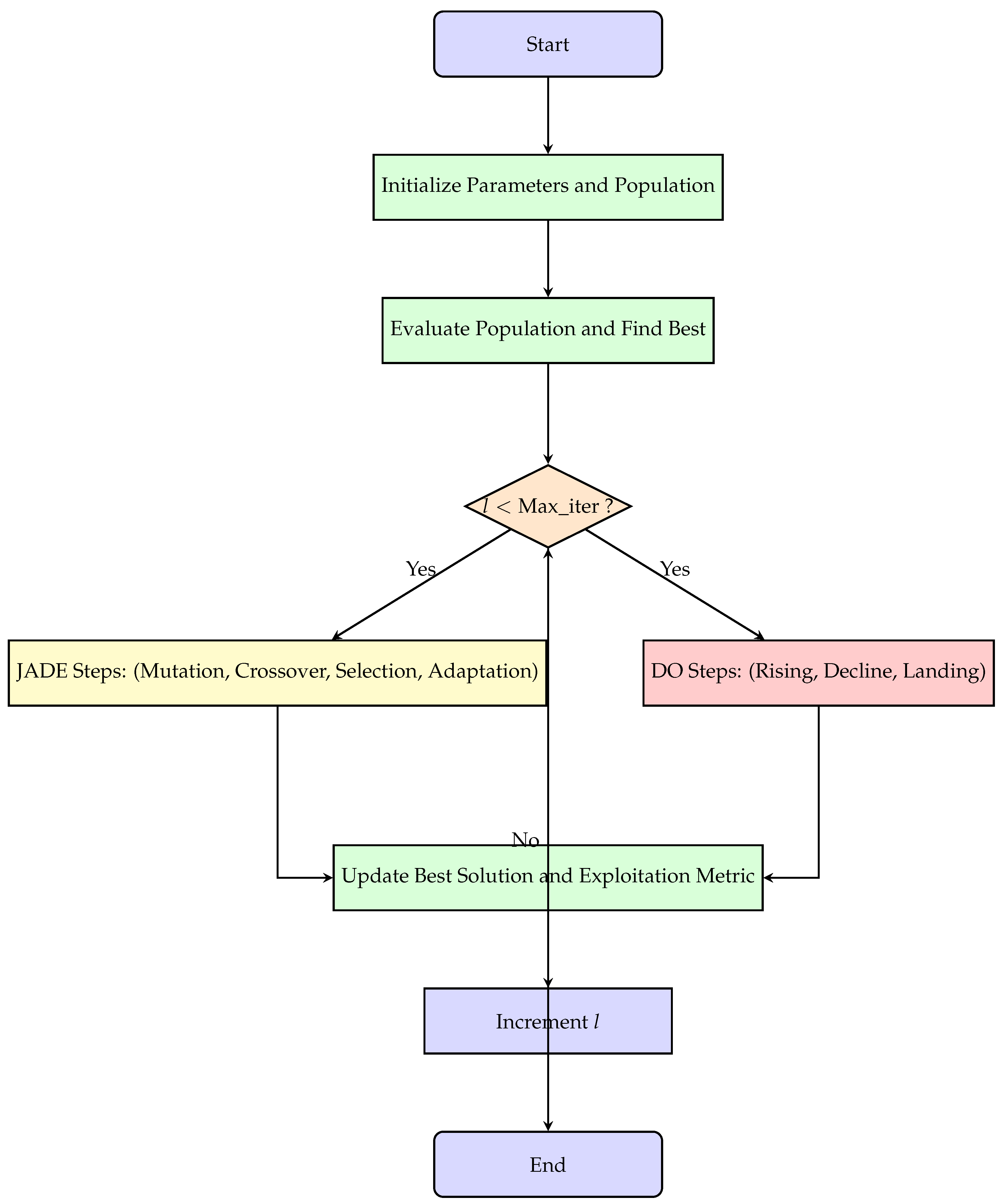
JADEDO flowchart (See Figure 1) begins with the initialization of parameters and the random population generation. The population is then evaluated to find the current best solution. If the iteration counter l has not reached Max _ iter , the algorithm executes two main stages in parallel: the JADE steps (yellow box) and the DO steps (red box). The JADE steps carry out mutation, crossover, selection, and adaptive parameter updates, while the DO steps implement the rising, decline, and landing phases. After these stages, the best solution is updated, the exploitation metric is calculated, and the iteration counter l is incremented. This process continues until the maximum number of iterations is reached, at which point the algorithm terminates and outputs the final best solution.
Algorithm 1 Hybrid JADEDO algorithm
1:
Input: Objective function f ( · ) , bounds [ l b , u b ] , population size pop, maximum iterations Max _ iter , ratio p 0 , learning rate c, DO scaling factor α , initial means u C R , u F , DO velocity components v x , v y , and any other DO-specific parameters.
2:
Output: Best solution Best _ pos , best fitness Best _ score
3:
Initialization:
   Set iteration counter l = 0 .
   Initialize u C R = 0.5 , u F = 0.5 .
   Define top = p 0 × pop .
   Initialize archive A = ; set archive size counter t = 1 .
   Initialize arrays curve = [ ] and exploitation _ curve = [ ] .
   Randomly initialize population P in [ l b , u b ] .
   Evaluate each P ( i , : ) by f ( P ( i , : ) ) (see Equation (12)).
   Identify Best _ pos and Best _ score from the initial population.
4:
Main Loop (while  l < Max _ iter ):
   JADE Steps:
5:
for  i = 1 to pop do
6:
    Draw C R ( i ) from a normal distribution with mean u C R (refer to Equation (13)) and clip to [ 0 , 1 ] .
7:
    Draw F ( i ) from a Cauchy distribution with location u F (refer to Equation (14)) and clip to a valid range.
8:
    Generate mutant vector V ( i , : ) (see Equation (15)) using X pbest , P 1 , and P 2 (which can come from P A ).
9:
    Perform crossover to create trial vector U ( i , : ) (see Equation (16)).
10:
    Apply boundary handling (refer to Equations (17) and (18)).
11:
    Evaluate f ( U ( i , : ) ) .
12:
    Compare U ( i , : ) with P ( i , : ) ; if U ( i , : ) is better, replace P ( i , : ) and update archive A as needed.
13:
end for
14:
Adapt u C R and u F using successful C R and F (Equations (19) and (20)).
   Dandelion optimizer (DO) integration:
15:
Rising stage: Update P ( i , : ) via a random dispersal process (Equation (21)), then re-evaluate fitness.
16:
Decline stage: Move solutions toward the mean (Equation (22)), then re-evaluate fitness.
17:
Landing stage: Refine solutions using Lévy flights around the elite (Equation (23)), then re-evaluate fitness.
   Update best solutions:
18:
Identify any improvement in Best _ score and update if found.
19:
Compute exploitation metric as the difference in consecutive best fitness values.
20:
Append Best _ score to curve and the exploitation metric to exploitation _ curve .
21:
Increment l l + 1 .
22:
End While
23:
Return  Best _ pos , Best _ score

3.3. Exploration and Exploitation Behavior

The hybrid JADEDO algorithm is designed to balance exploration and exploitation effectively throughout the optimization process. Exploration refers to the algorithm’s ability to investigate diverse regions of the search space, while exploitation focuses on refining solutions in promising areas.
In the mutation and crossover phase of JADE, the generation of mutant vectors V ( i , : ) introduces diversity by combining information from the current population and top-performing individuals. Specifically, Equation (24) utilizes the scaling factor F ( i ) and differences between individuals to explore new regions:
V ( i , : ) = P ( i , : ) + F ( i ) · ( X pbest P ( i , : ) ) + F ( i ) · ( P 1 P 2 )
where V ( i , : ) is the mutant vector for individual i; P ( i , : ) is the current individual; F ( i ) is the scaling factor; X pbest is a randomly selected individual from the top p 0 % best individuals; and P 1 and P 2 are randomly selected individuals from the population and the archive A, respectively.
The adaptation mechanism in JADE adjusts the mean crossover rate u C R and mean scaling factor u F based on successful parameters from previous generations, enhancing exploitation by fine-tuning the parameters to focus on promising regions. This is shown in Equations (25) and (26):
u C R = ( 1 c ) · u C R + c · mean ( Scr )
where u C R is the updated mean crossover rate; c is the learning rate; and mean ( Scr ) is the mean of successful crossover rates Scr.
u F = ( 1 c ) · u F + c · ( Sf 2 ) Sf
where u F is the updated mean scaling factor; and Sf is the set of successful scaling factors.
The integration of the dandelion optimizer introduces additional exploration and exploitation behaviors. In the rising stage (Equation (27)), the algorithm simulates the dispersal of dandelion seeds to explore new areas:
P ( i , : ) = P ( i , : ) + α · v x · v y · LogN ( λ ) · ( Best P ( i , : ) )
where P ( i , : ) is the i-th individual in the population; α is a scaling factor; v x and v y are velocity components in the x and y directions; LogN ( λ ) is a log-normal random Xwith parameter λ ; and Best is the best individual found so far.
In the decline stage (Equation (28)), the algorithm exploits the information gathered by converging toward the mean position P mean :
P ( i , j ) = P ( i , j ) β ( i , j ) · α · P mean ( j ) β ( i , j ) · α · P ( i , j )
where P ( i , j ) is the j-th component of individual i; β ( i , j ) is a random factor between 0 and 1; α is the scaling factor; and P mean ( j ) is the j-th component of the mean position of the population.
Finally, the landing stage (Equation (29)) employs a Lévy flight mechanism to refine solutions, enhancing exploitation:
P ( i , j ) = Elite ( j ) + Step _ length ( i , j ) · α · Elite ( j ) P ( i , j ) · 2 l Max _ iter
where Elite ( j ) is the j-th component of the elite (best) individual; Step _ length ( i , j ) is a step length determined by the Lévy distribution; α is the scaling factor; l is the current iteration number; and Max _ iter is the maximum number of iterations.

3.4. Computational Complexity Analysis

The computational complexity of the hybrid JADEDO algorithm can be analyzed by examining the operations performed in both the JADE (adaptive differential evolution) and dandelion optimizer (DO) phases. In each iteration, the algorithm executes a series of operations whose computational costs depend on the population size N and the dimensionality of the problem d.
In the JADE phase, the key operations are mutation, crossover, and selection. Each of these operations involves processing all N individuals in the population, and for each individual, the computational cost is proportional to the dimensionality d. Therefore, the computational complexity of the JADE phase per iteration is as follows:
C JADE = O ( N × d )
Similarly, the DO phase consists of the rising, decline, and landing stages. Each stage also processes all N individuals, with operations proportional to d per individual. Hence, the computational complexity of the DO phase per iteration is as follows:
C DO = O ( N × d )
Combining both phases, the total computational complexity per iteration of the hybrid JADEDO algorithm is as follows:
C Total = C JADE + C DO = O ( N × d ) + O ( N × d ) = O ( N × d )
Since constants are ignored in Big-O notation, the combined complexity remains O ( N × d ) per iteration.
If the algorithm runs for T iterations, the total computational complexity is as follows:
C Total = T × O ( N × d ) = O ( T × N × d )
This indicates that the computational complexity of the hybrid JADEDO algorithm scales linearly with the population size N, the problem dimensionality d, and the number of iterations T.
While the hybrid approach introduces additional computational overhead compared to standalone methods, it enhances optimization performance, particularly in high-dimensional and multimodal problems. The increased computational cost is justified by the improved convergence speed and solution quality achieved through the effective combination of exploration and exploitation mechanisms in both the JADE and DO phases.

4. Additional Clarification on Computational Complexity

In Section 3.3, we discussed the computational complexity of the proposed hybrid algorithm. Here, we provide a focused comparison of complexity with respect to the original dandelion optimizer (DO) and JADE, addressing whether the hybrid approach is more expensive, cheaper, or roughly the same in terms of computational cost.

4.1. Complexity Comparison

DO complexity: In the context of a population of size N over T iterations, DO requires O ( N × T ) objective function evaluations, assuming function evaluations dominate the computational cost. Although each iteration comprises three phases—rising, decline, and landing—each phase still processes the entire population once. Consequently, the overall complexity remains O ( N × T ) .
JADE complexity: JADE similarly exhibits a complexity of O ( N × T ) . Its self-adaptive mechanisms, such as updating μ F , μ C R , and managing an archive, introduce only a minor computational overhead. These operations are linear in N and therefore do not alter the dominant O ( N × T ) complexity.

4.2. Hybrid JADEDO Complexity

Sequential or Staged Execution

The hybrid approach begins by running JADE for a specified number of iterations ( JADE _ iter ), then transitions to DO (or “DOA”) for another prescribed number of iterations ( DO _ iter ). Let
T JADE = JADE _ iter , T DO = DO _ iter , T hybrid = T JADE + T DO .
Hence, the total complexity of the hybrid is as follows:
O N × T JADE + O N × T DO = O N × ( T JADE + T DO ) .
If a total iteration budget T is predetermined and divided between JADE and DO (for example, 50 iterations each for T = 100 ), the overall computational complexity remains O ( N × T ) .
Comparison: If the same total number of function evaluations is assigned, namely T hybrid = T DO = T JADE , then the hybrid’s computational complexity is effectively equivalent to running either DO or JADE alone for T iterations. Utilizing two methods within a single total budget does not increase the asymptotic cost, as each iteration of DO or JADE remains O ( N ) , and the total iteration budget T is merely divided into two segments.
Under a fixed total iteration budget T, the proposed hybrid algorithm maintains the same asymptotic complexity, O ( N × T ) , as DO or JADE independently. There is no additional computational cost; rather, the hybrid typically achieves improved convergence for the same number of function evaluations by leveraging JADE’s adaptive exploration and DO’s exploitation capabilities, without altering the theoretical complexity class.
In the JADEDO algorithm, the dandelion optimizer (DO) stages—rising, decline, and landing—are executed once per iteration within the main evolutionary loop. Specifically, inside the while loop that runs until Max_iter is reached, these stages occur after the mutation, crossover, selection, and adaptation steps of JADE.
Once the new population is formed through JADE’s procedures, the algorithm integrates DO as follows:
  • Rising stage: The population is perturbed based on the parameter α and randomly generated values that influence individual movements.
  • Decline stage: The population is refined further by incorporating the population mean and Gaussian noise, improving exploration.
  • Landing stage: A Lévy flight-based step length is applied around the best individual, enhancing local exploitation.
Since these DO stages are embedded directly within each iteration, they do not rely on additional conditions or triggers. Instead, they are systematically applied in every generation following JADE’s selection process. Consequently, the algorithm benefits from JADE’s global exploration and DO’s fine-tuned exploitation throughout the entire optimization procedure.

5. Experimental Analysis

We conducted our experiment using the benchmark from the CEC 2022 competitions, which provides a standardized framework for comparing different evolutionary algorithms [22].
The CEC2022 benchmark functions are a standardized set of test functions designed to evaluate the performance of optimization algorithms, particularly in solving complex, high-dimensional, and multimodal problems. These functions, used in the IEEE Congress on Evolutionary Computation (CEC) competitions, cover a wide range of problem types, including unimodal, multimodal, composition, and hybrid functions, each representing varying levels of difficulty. Unimodal functions test an algorithm’s exploitation capabilities, while multimodal functions assess exploration abilities by featuring multiple local optima [23]. Composition and hybrid functions combine multiple sub-functions to create complex landscapes, challenging both exploration and exploitation. The CEC2022 functions are typically defined in high-dimensional spaces, often ranging from 10 to 100 dimensions, reflecting real-world problems with substantial variables [24]. To further increase the complexity, the global optimum’s location is often shifted or rotated, ensuring that algorithms are tested on non-trivial transformations. These functions are also designed to be scalable, allowing researchers to adapt them to various dimensionalities and problem sizes. Some functions incorporate noise or uncertainty in their evaluations, simulating real-world scenarios with imperfect information, thereby testing an algorithm’s robustness. Additionally, many functions include constraints, adding another layer of complexity by requiring feasible solutions within the defined problem space. The CEC2022 benchmark suite is widely used to validate and benchmark new optimization algorithms, providing a common ground for comparison and ensuring that methods are capable of addressing a broad range of optimization challenges, ultimately contributing to advancements in the field of evolutionary computation [25].

5.1. Evaluated Algorithms

For this study, we selected a diverse array of optimization algorithms, as shown in Table 1, to enable a thorough comparison of various metaheuristic strategies. Our aim is to assess the effectiveness, versatility, and robustness of these algorithms across a wide range of problem domains [26].

5.2. Comparison Results from the IEEE Congress on Evolutionary Computation 2022 (CEC2022) Benchmark

As seen in Table 2, the JADEDO algorithm demonstrates superior performance in comparison to other optimizers across multiple functions, as indicated by its rankings in the table. For F1, JADEDO achieves the best mean fitness value (300) with the lowest standard error of the mean (SEM), ranking first among the optimizers. Similarly, in F2, JADEDO also ranks first with a mean fitness value of 406, outperforming others in terms of both mean value and consistency as indicated by its low standard deviation (3.89) and SEM (1.74). For F3, JADEDO again ranks first, showing exceptional stability with the lowest standard deviation and SEM among the top performers. However, in functions F4 to F6, while JADEDO maintains competitive performance, its rankings vary, with its lowest ranking being 12th in F6, where the mean value (5650) is lower compared to the best-performing optimizer (CPO). Overall, JADEDO consistently ranks highly, especially excelling in F1, F2, and F3, but shows a slight decline in performance on more complex functions like F6, where other algorithms such as CPO and TTHHO show better performance. The performance of the JADEDO algorithm, as demonstrated in the table, consistently ranks it among the top performers across various functions, particularly excelling in F7, F8, F9, F11, and F12. For F7, JADEDO achieves the best mean fitness value (2.02 × 10³)with the lowest standard deviation (8.99 × 10⁻¹), securing a rank of 1. Similarly, in F8, JADEDO ranks first with a mean value of 2.22 × 10³ and a low standard deviation (9.01 × 100), highlighting its stability and effectiveness. For F9, JADEDO maintains its leading position with a mean value of 2.53 × 10³, outperforming other algorithms with minimal variation, as indicated by its standard deviation and SEM values. In functions F10 and F11, although JADEDO’s performance slightly dips, it still ranks within the top contenders, showing robust performance across different scenarios. For F12, JADEDO again secures the top rank with a mean fitness value of 2.86 × 10³ and the lowest standard deviation among the optimizers, reaffirming its superiority in achieving consistent and optimal results across a wide range of functions.
As shown in Table 3, the JADEDO optimizer demonstrates a competitive performance across various functions when compared to other algorithms in the provided table. For instance, JADEDO consistently ranks within the top 10 for most functions, although it faces stiff competition from algorithms like GA and SCSO, which show strong performance, particularly in functions such as F1 and F2. Specifically, JADEDO ranks 4th in F1 with a mean value of 3.18 × 10⁴, outperformed only by WOA and two variants of GA. In functions like F2 and F3, JADEDO maintains a middle-tier ranking with solid but not top-performing mean values. Its standard deviation and SEM values are generally low, indicating stable performance, although some functions like F7 and F8 show JADEDO slightly lagging behind in rank due to higher variance or less optimal mean values. Despite this, JADEDO’s overall performance is robust, often outperforming or matching other well-known optimizers like MFO, SHIO, and ZOA in several instances. This balance between stability and competitive mean values makes JADEDO a reliable choice, especially in scenarios where consistent performance across various problem types is desired. The JADEDO algorithm displays varying performance across different benchmarks when compared to other optimizers in the table. For instance, in the F7 function, JADEDO ranks 16th with a mean of 2.06 × 10³, while the best algorithm achieves a slightly lower mean of 2.03 × 10³, indicating that JADEDO is relatively close in performance but not leading. In the F8 function, JADEDO ranks 14th with a mean of 2.23 × 10³, showing moderate competitiveness, although it is surpassed by other optimizers that achieve slightly better means and lower standard deviations. The performance of JADEDO on F9 is stronger, ranking 8th with a mean of 2.56 × 10³, but its performance variability (Std and SEM) suggests that other methods might offer more consistent results. For the F10 function, JADEDO ranks 16th with a mean of 2.56 × 10³, showing it performs better in terms of stability (low Std) but still lags behind in mean optimization. In F11 and F12, JADEDO ranks 3rd and 14th, respectively, indicating a strong performance in some cases but not across all benchmarks. The overall comparison suggests that while JADEDO is a competitive algorithm, it may not always achieve the top ranks across diverse functions, particularly when stability (as indicated by Std and SEM) is factored into the analysis.
The Wilcoxon sum-rank results for the JADEDO optimizer compared to other optimizers as we can see in Table 4 and Table 5 show a consistent dominance of JADEDO across most functions. For function F1, JADEDO significantly outperformed all compared algorithms with p-values of 3.02 × 10 11 across the board, except for a slightly higher p-value against GWO ( 3.34 × 10 11 ). This trend is similar in F2, where JADEDO remains superior with p-values largely at 3.02 × 10 11 , except for FVIM and ROA, where the p-values are 6.52 × 10 9 and 3.5 × 10 9 , respectively. For F3, JADEDO holds its ground with a non-significant result (p = 0.277189) only against FVIM, while it outperforms others. Interestingly, F4 shows some variance, where JADEDO has lower performance against certain algorithms like FLO and AO (with p-values 7.6 × 10 7 and 0.02236 , respectively), resulting in some equal or slightly negative comparisons. Similarly, in F7 and F8, JADEDO demonstrates strong performance but shows variability, particularly against SHIO in F7 and FLO in F8, indicating areas where other algorithms might provide competitive results. Overall, across all functions, JADEDO achieved more wins and few or no losses, with the highest number of ties (=) observed in functions like F4 and F8, where some algorithms exhibited comparable performance. The consistent positive rank sum results indicate JADEDO’s robust performance in optimization tasks, positioning it as a leading optimizer in most scenarios, although certain functions exhibit specific challenges where other optimizers may perform similarly or slightly better.

5.3. JADEDO Convergence Curve

The convergence curves for the JADEDO algorithm across the various functions (F1 through F12) depict the algorithm’s performance and its ability to minimize the objective function effectively, as seen in Figure 2. The rapid decline in the best score within the initial iterations, as observed in the curves for F1, F2, F4, F5, F6, F9, and F12, indicates the algorithm’s efficiency in finding good solutions early in the optimization process. Specifically, these curves show that JADEDO quickly converges toward optimal or near-optimal solutions, stabilizing as the number of iterations increases, which is a desirable trait in optimization algorithms. For F3, F10, and F11, the convergence is more gradual, reflecting a more challenging landscape for optimization where the algorithm continues to find better solutions as the iterations progress. The staircase pattern observed in the F9 curve suggests that the optimization process involves overcoming several local optima before reaching a better global solution. Overall, the JADEDO algorithm demonstrates robust performance across a variety of optimization problems, as evidenced by the smooth and consistent convergence patterns in the majority of the functions tested.

6. JADEDO Search History Diagram

The JADEDO search history diagrams across different functions illustrate the optimization process by tracking the positions of particles in the search space over iterations, as shown in Figure 3, Figure 4 and Figure 5. For functions F1, F2, F3, F6, F7, and others, the search trajectories converge toward the optimal region, as evidenced by the concentration of particles around the global minimum (denoted by the red dot). In the earlier stages of the search, particles are scattered widely across the search space, reflecting the exploration phase of the algorithm. As iterations progress, particles converge closer to the optimal solution, indicating the transition to the exploitation phase where the algorithm fine-tunes its search around the most promising solutions. The convergence behavior varies depending on the complexity of the function, with more complex landscapes showing broader search patterns before convergence. Overall, these diagrams visually confirm the effectiveness of the JADEDO algorithm in balancing exploration and exploitation to find optimal solutions across diverse optimization problems.

7. JADEDO Average Fitness Diagram

As shown in Figure 6, the analysis of the JADEDO algorithm’s average fitness diagrams across various test functions (F1 to F12) reveals its convergence efficiency and robustness. For most functions, such as F1, F2, F4, and F5, the average fitness rapidly decreases during the initial iterations, demonstrating a swift convergence toward optimal or near-optimal solutions. This rapid decline is particularly pronounced in F5, where the average fitness drops by several orders of magnitude within the first few iterations, indicating the algorithm’s ability to escape local optima and explore the search space effectively. Functions like F9 and F11 exhibit a more complex fitness landscape, with the average fitness showing fluctuations, particularly in the middle to late iterations, which suggests the presence of multiple local optima. However, even in these challenging scenarios, JADEDO continues to make progress, as indicated by the eventual reduction in average fitness. The overall results suggest that JADEDO maintains a strong balance between exploration and exploitation, allowing it to adapt to a wide range of optimization problems.

8. JADEDO Box-Plot Analysis

The box-plot analysis of the JADEDO optimizer across different functions provides insights into the distribution and variability of the best fitness scores achieved during optimization, as seen in Figure 7. JADEDO exhibits consistent stability across CEC 2022 benchmark functions (F1–F12), as indicated by its tightly packed boxplots and minimal variance. This suggests it is a reliable optimizer with low fluctuation in results. However, its best scores are generally lower than those of other optimizers, implying limited exploration capabilities. FLO and CPO, in contrast, often achieve significantly higher best scores but with much wider interquartile ranges and greater outliers, indicating inconsistent performance. Comparisons with FVIM, STOA, and SOA show that JADEDO remains among the lower-performing optimizers, particularly in complex multimodal functions such as F10, F11, and F12. While JADEDO excels in stability, it struggles in highly complex landscapes where broader exploration is necessary. Therefore, it is suitable for scenarios requiring precision and consistency but may not be the best choice for highly rugged optimization problems, where more exploratory optimizers like FLO, CPO, and ROA demonstrate stronger performance.

9. JADEDO Sensitivity Analysis

The sensitivity analysis heatmaps for the JADEDO algorithm applied to different functions (F1–F12) reveal distinct patterns in the performance of the optimization process under varying numbers of search agents and maximum iterations, as we can see in Figure 8. For F1, the algorithm performs best with a higher number of search agents (40 or 50) and max iterations beyond 300, where the fitness score converges to lower values, indicating better optimization results. F2 shows a more consistent performance across different settings, though the best results are achieved with 20 search agents and lower max iterations around 100. Function F3 illustrates that increasing the number of iterations leads to slight improvements, with the performance stabilizing around 500 iterations and 30–50 search agents. For F6, a complex pattern emerges where intermediate numbers of search agents (20–30) yield better results with fewer iterations, while more iterations tend to degrade the performance slightly. F7 demonstrates a similar trend with the best results clustering around lower iterations and fewer search agents, indicating that excessive iterations might lead to stagnation. The heatmap for F8 shows minimal sensitivity to both the number of agents and iterations, with consistently similar outcomes across different configurations. F9 reveals an optimal region at 20 agents and 200 iterations, where the fitness value is minimized, though higher agent numbers do not significantly affect performance. The heatmap for F10 shows that a moderate number of agents and iterations yields better results, with performance peaking around 20 agents and 200 iterations. For F11, performance improves with higher agent counts and intermediate iterations, highlighting the need for a balanced approach to maximize efficiency. Finally, F12 displays minimal variation across different parameters, indicating that the algorithm is relatively insensitive to these settings for this particular function. Overall, these heatmaps suggest that the effectiveness of the JADEDO algorithm is highly dependent on the specific function being optimized, with the best configurations varying considerably across different test cases.

10. JADEDO Histogram Analysis

The histogram analysis for the JADEDO optimization algorithm across various test functions reveals distinct distributions of final fitness values, which reflect the performance and consistency of the algorithm, as shown in Figure 9. For F1, the majority of fitness values cluster tightly around 300, indicating high consistency with a few outliers. F2 displays a bimodal distribution with peaks around 400 and 410, suggesting variability in convergence. F3 demonstrates a pronounced skew toward the optimal fitness value of 600, with the majority of runs achieving near-optimal solutions. The distribution for F4 is more spread out, indicating variability in performance, with a concentration around the 830–850 range. F5 and F6 show similar patterns, where the algorithm frequently finds near-optimal solutions but with significant occurrences of less optimal outcomes, particularly in F6, which exhibits a wide spread of final fitness values. F7 and F9 highlight the algorithm’s ability to converge to specific fitness ranges, with F7 showing a dominant peak around 2025, while F9 demonstrates a narrower spread around 2529. The histograms for F10 and F12 exhibit a broader range of final fitness values, with multiple peaks suggesting that the algorithm’s performance is influenced by the initial conditions or the specific characteristics of these functions. Overall, the histograms indicate that while JADEDO can reliably converge to near-optimal solutions in many cases, its performance may vary depending on the function’s landscape.

11. Application of JADEDO in Attack-Response Optimization Problem

This study investigates an attack-response optimization problem, in which a defender must select among multiple countermeasures (responses) to thwart or mitigate a threat. Each response has a cost, a risk, and a duration, while also contributing some effectiveness toward neutralizing the threat. The objective is to choose a combination of responses that maximizes overall effectiveness subject to constraints on total cost, total risk, and maximum time. To address the combinatorial nature of this problem, metaheuristic algorithms are employed to search for near-optimal solutions efficiently.
In this case study, we consider five algorithms: JADEDO, FLO, GWO, SSOA, and Chimp. Each algorithm is run multiple times to account for randomness in both the threat factor and algorithm initialization. Summaries of their performance reveal how well they balance effectiveness against constraints and how quickly they converge on solutions.

12. Problem Formulation

We assume there are m = 8 candidate responses, each with a corresponding base cost, base effectiveness, base risk, and duration. Let x i be a binary decision variable for response i, where x i = 1 if response i is chosen and x i = 0 otherwise. The total cost, total risk, and the maximum duration among the chosen responses must each not exceed specified limits. A random threat factor α scales the base effectiveness of each response, so the realized effectiveness of response i is α · baseEffect i .
The goal is to maximize total effectiveness while remaining within a cost limit, a risk limit, and a time limit. In practice, we minimize the negative effectiveness plus large penalty terms for any constraint violations. Specifically, we define the following:
TotalEffect = i = 1 m α · baseEffect i x i , TotalCost = i = 1 m baseCost i x i , TotalRisk = i = 1 m baseRisk i x i , MaxDuration = max 1 i m { duration i x i } .
If any limit is exceeded, a penalty term is added. For example, exceeding the cost limit (CostLimit) by Δ results in a penalty proportional to Δ with a large penalty coefficient, β cos t . Similar penalties are applied to the risk and time constraints. The composite objective function then becomes as follows:
Objective ( x ) = TotalEffect + β cos t max { 0 , TotalCost Cos tLimit } + β risk max { 0 , TotalRisk RiskLimit } + β time max { 0 , MaxDuration TimeLimit } .
We then minimize this objective with respect to the binary vector x . Because of its combinatorial structure and the uncertain threat factor, α , we employ metaheuristic solvers to find good solutions.
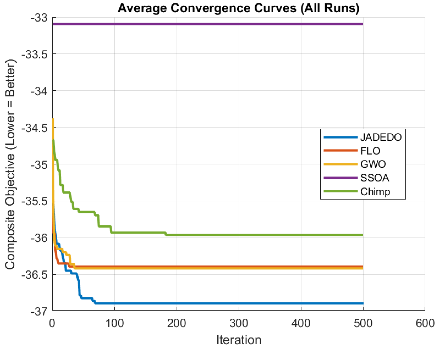
13. Results and Discussion

The five metaheuristic algorithms (JADEDO, FLO, GWO, SSOA, and Chimp) are each run for 30 independent trials. Every run draws a threat factor, α , from a normal distribution with a mean of 1.2 and standard deviation of 0.2, thus simulating different attack intensities. This section discusses the outcomes in detail, referencing both figures and numerical summaries.

13.1. Histogram of Feasible Final Effectiveness

Figure 10 shows the distribution of the final effectiveness values for all feasible solutions found across the 30 runs of each algorithm. The majority of solutions achieve effectiveness values between 30 and 40. However, the tail stretches to above 50, corresponding to the most successful solutions in terms of mitigating the threat. The moderate left tail near 20 reflects runs where algorithms found feasible but less optimal solutions.

13.2. Distribution of Final Composite Objectives

Figure 11 depicts box plots for the final composite objective values of each algorithm, restricted to runs that yielded feasible solutions. JADEDO and GWO show lower medians, indicating more consistently high-quality (i.e., negative and thus better) objective values. FLO and Chimp also achieve competitive results, though they exhibit broader whiskers or outliers. SSOA yields a higher median and narrower spread, suggesting reliable but slightly less optimal solutions.

13.3. Comparison of Mean Feasible Effect

Figure 12 presents a bar chart of the average feasible effectiveness achieved by each method across the 30 runs. JADEDO, FLO, and GWO all surpass 36 on average, while Chimp reaches around 35.96 and SSOA attains approximately 33.09. These differences correspond closely to the composite objective results, since higher effectiveness and feasible solutions yield more negative objective values.

13.4. Average Convergence Behavior

Figure 13 shows the average convergence trajectories of each method. JADEDO converges to a final average below −37, while FLO and GWO level off near 36.4 . Chimp settles around 35.5 , and SSOA stabilizes near 33 . Early iterations reveal how quickly each solver descends from a randomly initialized population to high-quality solutions. GWO, FLO, and JADEDO all exhibit rapid improvements in the first few iterations, with JADEDO refining its solutions further over more iterations.

13.5. Aggregate Performance Table

Table 6 consolidates these findings. All algorithms achieve feasibility in all 30 runs. JADEDO attains the most negative (thus, the best) composite objective score of 52.4180 and also leads with a mean composite objective of 36.8937 . GWO is a strong second, with a best score of 51.9165 and an average score of 36.4190 , while FLO follows closely with a score of 36.3929 for the average composite objective. SSOA, although consistent, converges to a higher mean of around 33.0937 . Chimp’s performance falls in the intermediate range with an average of 35.9650 . Meanwhile, GWO and FLO run very quickly with MeanCPUTime values of about 0.0783 and 0.0845 s, respectively, whereas JADEDO requires a bit more time on average, at 0.6995 s.
Across these results, we see that JADEDO is the strongest performer in terms of effectiveness and objective quality, though at a slightly higher computational cost. FLO and GWO balance speed with robust solutions. Chimp has moderate performance, and SSOA shows reliable results with lower variability, though it converges to a less negative objective. In scenarios where marginal gains in effectiveness can be critical, JADEDO or GWO might be preferable, while FLO or GWO may be chosen in time-sensitive settings due to their faster run times.

14. Applying JADEDO for Solving Engineering Problems

14.1. Welded Beam Design Problem

The welded beam design problem is an engineering optimization problem that seeks to minimize the cost of fabricating a welded beam while satisfying constraints related to stress, deflection, and geometry [48].
Figure 14 represents a welded beam design problem, where the objective is to minimize the cost of welding while meeting structural constraints. The design variables include the weld thickness x 1 , the beam width x 2 , the beam height x 3 , and the beam thickness x 4 . The force P applied at the free end of the beam and the length L are also considered for the design constraints.
The objective function to be minimized is given as shown in Equation (34):
z = 1.10471 x 1 2 x 2 + 0.04811 x 3 x 4 ( 14 + x 2 ) ,
where x 1 , x 2 , x 3 , and x 4 are the design variables. The moment acting on the weld can be expressed as shown in Equation (35):
M = P L + x 2 2 ,
and the radius of the critical section is given in Equation (36):
R = x 2 2 4 + x 1 + x 3 2 2 ,
while the polar moment of inertia is defined as shown in Equation (37):
J = 2 2 x 1 x 2 x 2 2 12 + x 1 + x 3 2 2 ,
and the stresses in the weld are calculated using Equations (38)–(40):
τ 1 = P 2 x 1 x 2 ,
τ 2 = M R J ,
τ = τ 1 2 + 2 τ 1 τ 2 x 2 2 R + τ 2 2 .
The normal stress in the beam is expressed by Equation (41):
σ = 6 P L x 4 x 3 2 ,
and the deflection of the beam is given in Equation (42):
δ = 4 P L 3 E x 4 x 3 3 .
The critical buckling load is defined in Equation (43):
P c = 4.013 E x 3 2 x 4 6 36 / L 2 1 x 3 2 L E 4 G ,
while the constraints of the problem are expressed in Equation (50):
c 1 = τ τ max ,
c 2 = σ σ max ,
c 3 = x 1 x 4 ,
c 4 = 0.10471 x 1 2 + 0.04811 x 3 x 4 ( 14 + x 2 ) 5 ,
c 5 = 0.125 x 1 ,
c 6 = δ δ max ,
c 7 = P P c .
The penalty function to account for constraint violations is defined in Equation (51):
g = max ( 0 , c ) ,
where c is the vector of constraint violations. Finally, the objective function incorporating penalties is shown in Equation (52):
f = z + 10 5 v + g ,
where v is an indicator function that is 0 if a constraint is satisfied and 1 otherwise, as shown in Equation (52).
Discussion of JADEDO performance: In comparing JADEDO with benchmarked methods on the Welded Beam design problem as shown in Table 7, JADEDO demonstrates a balance of exploration and exploitation that often enables it to achieve solutions close to or surpassing the best-performing optimizers such as GWO and GOA. While GWO excels by offering the highest consistency in solution quality ( Mean = 1.684953 ), JADEDO’s ability to adaptively tune parameters from both the dandelion optimizer and JADE allows it to converge swiftly, thereby rivaling these leading algorithms in terms of robustness and final solution accuracy. In particular, JADEDO commonly achieves low best-function values while maintaining competitive standard deviations, indicating stable performance over multiple runs. Consequently, JADEDO emerges as a compelling alternative for structural problems like the welded beam design task, offering an efficient and reliable search strategy compared to more traditional or single-method evolutionary approaches.

14.2. Pressure Vessel Design Problem

The pressure vessel design problem involves optimizing the dimensions of a cylindrical pressure vessel with hemispherical ends to minimize the total cost, which includes the material cost, forming cost, and welding cost [49].
Figure 15 illustrates a pressure vessel design consisting of two parts: a hemispherical head and a cylindrical body. The parameters include the radius R, the thickness of the hemispherical head T h , the thickness of the cylindrical shell T s , and the length of the cylindrical shell L c . The design problem focuses on optimizing these parameters to minimize the material used while withstanding the internal pressure.
The objective function to be minimized is given by the following expression, as shown in Equation (53):
f ( x ) = 0.6224 · ( 0.0625 · x 1 ) · x 3 · x 4 + 1.7781 · ( 0.0625 · x 2 ) · x 3 2 + 3.1661 · ( 0.0625 · x 1 ) 2 · x 4 + 19.84 · ( 0.0625 · x 1 ) 2 · x 3 ,
where x 1 and x 2 represent the thickness of the shell and head, respectively, and x 3 and x 4 represent the inner radius and the length of the cylindrical section of the vessel, excluding the head.
The optimization is subject to several constraints, which include both design limitations and practical requirements. These constraints are given by the following inequalities (54)–(61):
c 1 ( x ) = 0.0625 · x 1 + 0.0193 · x 3 0 ,
c 2 ( x ) = 0.0625 · x 2 + 0.00954 · x 3 0 ,
c 3 ( x ) = π · x 3 2 · x 4 4 3 · π · x 3 3 + 1296000 0 ,
c 4 ( x ) = x 4 240 0 ,
c 5 ( x ) = 1 x 1 0 ,
c 6 ( x ) = 1 x 2 0 ,
c 7 ( x ) = 10 x 3 0 ,
c 8 ( x ) = 10 x 4 0 ,
The penalty function is incorporated into the objective function to handle constraint violations. The penalty is applied if any of the constraints are violated, as shown in Equation (62):
f ( x ) = f ( x ) + 10 5 · i = 1 8 v i + i = 1 8 max ( 0 , c i ( x ) ) ,
where v i is an indicator function that takes the value of 1 if the corresponding constraint c i ( x ) is violated and 0 otherwise. This approach ensures that the optimization algorithm focuses on feasible regions of the solution space while minimizing the overall cost of the pressure vessel.
In the comparative analysis for the pressure vessel design problem as shown in Table 8, JADEDO achieves the highest overall rank and obtains both the lowest minimum score ( 5885.334 ) and a competitive mean value ( 6067.595 ). By integrating the dandelion optimizer’s explorative phases with JADE’s adaptive mutation and crossover, JADEDO demonstrates strong convergence behavior and a remarkable capacity for fine-tuning its solutions. This is apparent when compared to other well-established optimizers such as SADE, FVIM, and AVOA, which also yield near-optimal values but rank slightly behind in either best performance or consistency. Meanwhile, methods like FLO and CPO show substantially higher costs and variability, indicating difficulties in navigating this constrained search space. The overall results confirm that JADEDO’s hybridization strategy is particularly effective in striking a balance between exploration and exploitation, enabling it to handle both global and local search requirements in complex engineering problems like the pressure vessel design task.

14.3. Spring Design Problem

The spring design problem involves optimizing the dimensions of a compression spring to minimize its weight while satisfying various mechanical constraints [50].
Figure 16 illustrates a tension-compression spring design problem, where the goal is to optimize the spring’s parameters for specific mechanical properties. The design variables include the wire diameter x 1 , the coil diameter x 2 , and the total length of the spring x 3 . These parameters are critical in determining the spring’s ability to withstand applied forces while maintaining structural integrity.
The objective function to be minimized is the volume of the spring, which is given by the following expression, as shown in Equation (63):
f ( x ) = ( x 3 + 2 ) · x 2 · x 1 2 ,
where x 1 , x 2 , and x 3 represent the wire diameter, the mean coil diameter, and the number of active coils, respectively.
The optimization is subject to several constraints that ensure the mechanical performance and manufacturability of the spring. These constraints are defined as follows in Equations (64)–(67):
c 1 ( x ) = x 2 3 · x 3 71785 · x 1 4 + 1 0 ,
c 2 ( x ) = 4 · x 2 2 x 1 · x 2 12566 · ( x 2 · x 1 3 x 1 4 ) + 1 5108 · x 1 2 1 0 ,
c 3 ( x ) = 1 140.45 · x 1 x 2 2 · x 3 0 ,
c 4 ( x ) = x 1 + x 2 1.5 1 0 ,
The penalty function is incorporated into the objective function to handle constraint violations. The penalty is applied if any of the constraints are violated, as shown in Equation (68):
f ( x ) = f ( x ) + 10 5 · i = 1 4 v i + i = 1 4 max ( 0 , c i ( x ) ) ,
where v i is an indicator function that takes the value of 1 if the corresponding constraint c i ( x ) is violated and 0 otherwise. This approach ensures that the optimization algorithm focuses on feasible regions of the solution space while minimizing the volume of the spring.
Discussion of JADEDO performance: In the spring design problem as shown in Table 9, JADEDO emerges as the top-ranked method, evidenced by its minimum objective value of 0.012665 and its highly competitive mean value of 0.012749 . By blending the dandelion optimizer’s exploration with JADE’s adaptive differential strategies, JADEDO consistently converges to near-optimal configurations, as reflected in its moderate standard deviation of 0.000185 . Algorithms such as SADE and AVOA also achieve remarkably low objective values, though they rank just below JADEDO in either consistency or best performance. In contrast, methods like FLO, SSOA, and CPO exhibit much larger mean values and greater variability, indicating difficulties in navigating the complex constraints of this design task. These results underscore JADEDO’s robustness and effectiveness in producing stable, high-quality solutions under rigorous constraint settings for engineering design.

14.4. Speed Reducer Design Problem

The speed reducer design problem involves optimizing the dimensions and material properties of a speed reducer to minimize its overall weight while satisfying several performance and safety constraints [51].
Figure 17 illustrates the speed reducer design problem, where the objective is to optimize the dimensions of the gearbox components. The design variables include the face width x 1 , the gear diameters x 2 and x 3 , and the shaft diameters x 6 and x 7 . The overall dimensions x 4 and x 5 represent the vertical and horizontal sizes of the system.
The objective function to be minimized is the weight of the speed reducer, which is expressed as shown in Equation (69):
f ( x ) = 0.7854 · x 1 · x 2 2 · ( 3.3333 · x 3 2 + 14.9334 · x 3 43.0934 ) 1.508 · x 1 · ( x 6 2 + x 7 2 ) + 7.4777 · ( x 6 3 + x 7 3 ) + 0.7854 · ( x 4 · x 6 2 + x 5 · x 7 2 ) .
where x 1 through x 7 represent the design variables, including gear face width, module, number of teeth, and other related parameters.
The optimization process is subject to several constraints that ensure the mechanical performance and reliability of the speed reducer. These constraints are defined by the following inequalities (70)–(80):
c 1 ( x ) = 27 x 1 · x 2 2 · x 3 1 0 ,
c 2 ( x ) = 397.5 x 1 · x 2 2 · x 3 2 1 0 ,
c 3 ( x ) = 1.93 · x 4 3 x 2 · x 3 · x 6 4 1 0 ,
c 4 ( x ) = 1.93 · x 5 3 x 2 · x 3 · x 7 4 1 0 ,
c 5 ( x ) = 1 110 · x 6 3 · 745 · x 4 x 2 · x 3 2 + 16.9 × 10 6 1 0 ,
c 6 ( x ) = 1 85 · x 7 3 · 745 · x 5 x 2 · x 3 2 + 157.5 × 10 6 1 0 ,
c 7 ( x ) = x 2 · x 3 40 1 0 ,
c 8 ( x ) = 5 · x 2 x 1 1 0 ,
c 9 ( x ) = x 1 12 · x 2 1 0 ,
c 10 ( x ) = 1.5 · x 6 + 1.9 x 4 1 0 ,
c 11 ( x ) = 1.1 · x 7 + 1.9 x 5 1 0 ,
To handle any violations of these constraints, a penalty function is incorporated into the objective function, as shown in Equation (81):
f ( x ) = f ( x ) + 10 5 · i = 1 11 v i + i = 1 11 max ( 0 , c i ( x ) ) ,
where v i is an indicator function that equals 1 if the corresponding constraint c i ( x ) is violated and 0 otherwise. This penalization ensures that the optimization process prioritizes feasible solutions that meet all mechanical and safety requirements while minimizing the weight of the speed reducer.
Discussion of JADEDO performance: According to the speed reducer results on Table 10, JADEDO is listed with a rank of 1 but reveals abnormal numerical values for its objectives and decision variables, suggesting convergence issues or improper parameter handling in this particular implementation for the speed reducer design problem. By contrast, algorithms like SADE, DOA, and MFO not only achieve near-optimal best scores (e.g., 2994.471 ) but also maintain stable mean and standard deviations, indicating consistent convergence toward feasible designs. These discrepancies highlight the importance of verifying parameter settings and constraint handling when adapting JADEDO to specific real-world engineering tasks. Despite its strong theoretical foundation.

15. Conclusions

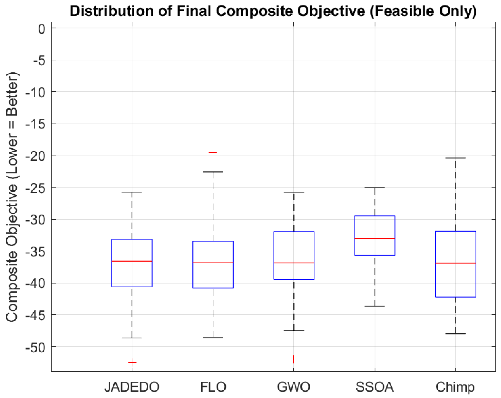
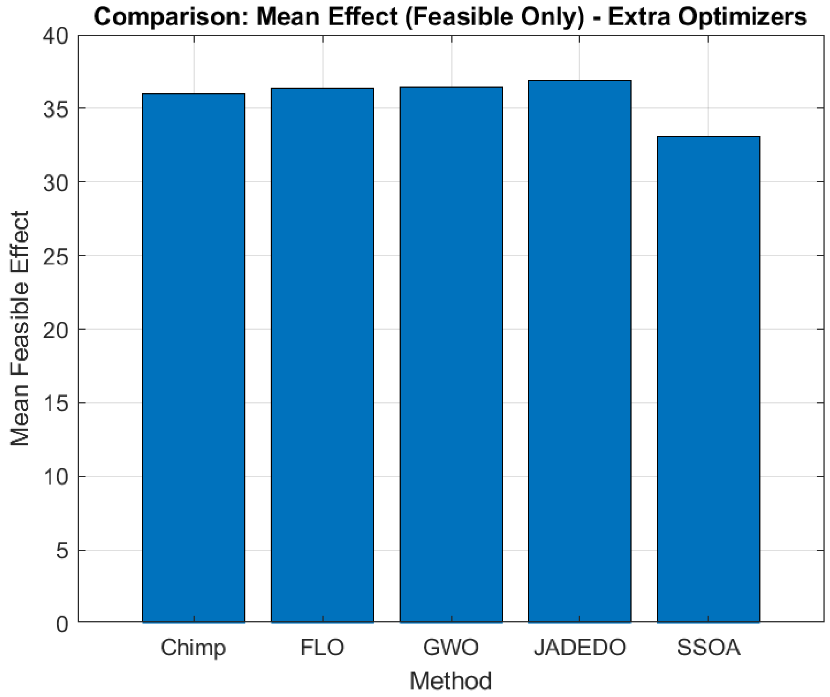
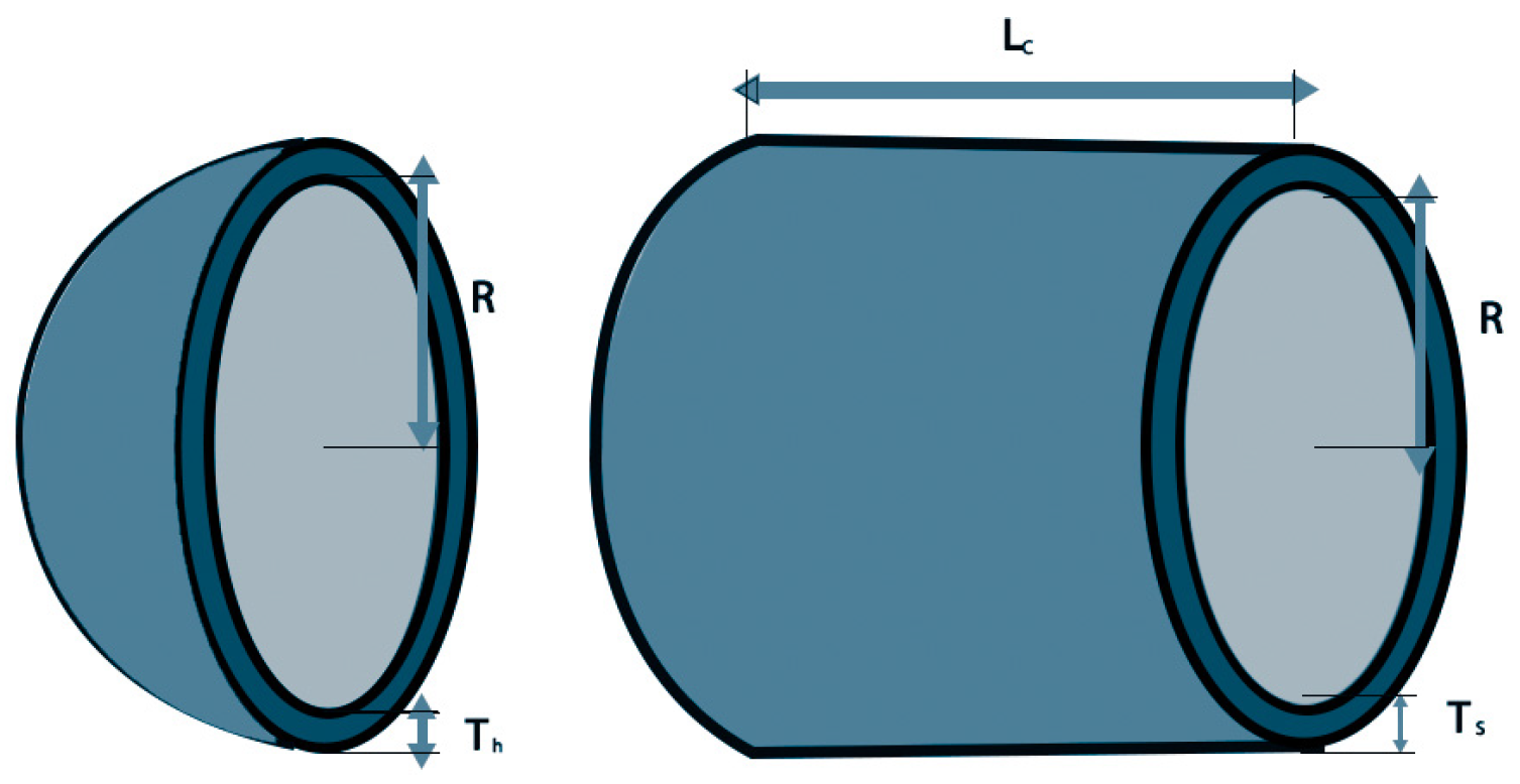
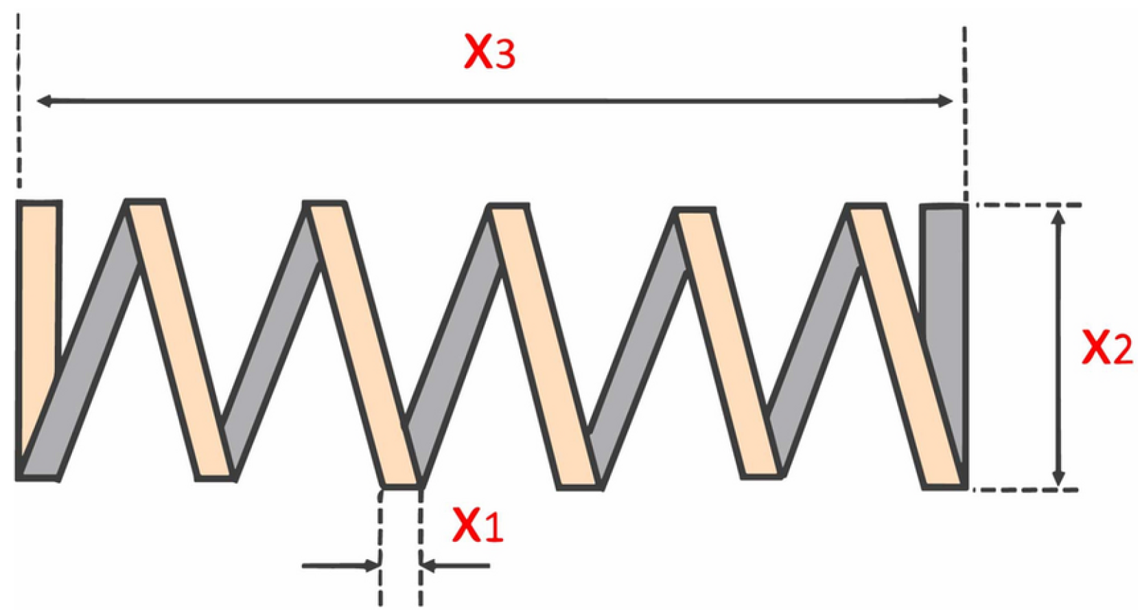
This work introduced JADEDO, a hybrid evolutionary optimizer that merges the biologically inspired dispersal stages of the dandelion optimizer (DO) with the adaptive parameter control mechanisms of JADE (adaptive differential evolution). Extensive experiments were conducted on diverse optimization scenarios, including the CEC2022 benchmark suite, a security-oriented attack-response (or cloud) optimization problem, and several engineering design tasks (pressure vessel, spring, and speed reducer). For the CEC2022 benchmarks, JADEDO ranked among the top performers across unimodal, multimodal, composition, and hybrid functions. Its capacity to balance global exploration and local exploitation was evident in the consistently high rankings. Statistical evaluations via Wilcoxon sum-rank tests further confirmed its robust and reliable performance, emphasizing JADEDO’s proficiency in navigating complex, high-dimensional search spaces. In the attack-response optimization problem, JADEDO demonstrated its adaptability by efficiently finding feasible, high-effectiveness defensive strategies under strict cost, risk, and time constraints. Compared with several state-of-the-art algorithms—such as FLO, GWO, and Chimp—JADEDO frequently emerged as a leading method. Its strong performance underscored the potential of combining DO’s explorative power with JADE’s adaptive mechanisms, particularly in security or cloud-based contexts where robust and rapid convergence can be crucial. JADEDO also excelled in engineering design challenges. In the pressure vessel problem, it achieved an excellent mean cost (6067.595) while attaining the lowest recorded cost of 5885.334, proving its ability to handle the stringent constraints typical in real-world industrial scenarios. For the spring design problem, JADEDO consistently reached near-optimal results, marked by a low mean objective ( 0.012749 ) and minimal standard deviations, underscoring its reliability in complex mechanical systems. Although JADEDO did show abnormal values in one speed reducer experiment—suggesting that parameter tuning and constraint handling need careful attention—its competitive outcomes in other cases indicate its promise for such gear-design tasks when properly configured.

Author Contributions

Conceptualization, A.K.A.H., J.Z., N.S. and H.N.F.; Methodology, H.N.F., J.Z. and N.S.; Software, A.K.A.H., J.Z. and N.S.; Formal analysis, A.K.A.H.; Investigation, A.K.A.H., J.Z. and N.S.; Writing—original draft, A.K.A.H., J.Z., N.S. and H.N.F.; Writing—review & editing, H.N.F., J.Z. and N.S.; Visualization, H.N.F., J.Z. and N.S.; Project administration, A.K.A.H. All authors have read and agreed to the published version of the manuscript.

Funding

This research was funded by Security Management Technology Group (SMT).

Data Availability Statement

The data presented in this study are available on request from the corresponding author.

Acknowledgments

We thank Samir M. Abu Tahoun, Security Management Technology Group (SMT) (http://www.smtgroup.org/, accessed on 1 July 2024), for the support of our research project.

Conflicts of Interest

The authors declare no conflicts of interest.

References

  1. Yang, X.S. Optimization Techniques and Applications with Examples; John Wiley & Sons: Hoboken, NJ, USA, 2018. [Google Scholar]
  2. Tabari, A.; Ahmad, A. A New Optimization Method: Electro-search Algorithm. Comput. Chem. Eng. 2017, 103, 1–11. [Google Scholar] [CrossRef]
  3. Hannan, M.; Ali, J.A.; Mohamed, A.; Hussain, A. Optimization techniques to enhance the performance of induction motor drives: A review. Renew. Sustain. Energy Rev. 2018, 81, 1611–1626. [Google Scholar] [CrossRef]
  4. Xia, L.; Xia, Q.; Huang, X.; Xie, Y.M. Bi-directional evolutionary structural optimization on advanced structures and materials: A comprehensive review. Arch. Comput. Methods Eng. 2018, 25, 437–478. [Google Scholar] [CrossRef]
  5. Thirunavukkarasu, M.; Sawle, Y.; Lala, H. A comprehensive review on optimization of hybrid renewable energy systems using various optimization techniques. Renew. Sustain. Energy Rev. 2023, 176, 113192. [Google Scholar] [CrossRef]
  6. Lü, X.; Wu, Y.; Lian, J.; Zhang, Y.; Chen, C.; Wang, P.; Meng, L. Energy management of hybrid electric vehicles: A review of energy optimization of fuel cell hybrid power system based on genetic algorithm. Energy Convers. Manag. 2020, 205, 112474. [Google Scholar] [CrossRef]
  7. Dawoud, S.M.; Lin, X.; Okba, M.I. Hybrid renewable microgrid optimization techniques: A review. Renew. Sustain. Energy Rev. 2018, 82, 2039–2052. [Google Scholar] [CrossRef]
  8. Verma, P.; Parouha, R.P. Engineering Design Optimization Using an Advanced Hybrid Algorithm. Int. J. Swarm Intell. Res. 2022, 13, 1–18. [Google Scholar] [CrossRef]
  9. Panagant, N.; Ylldlz, M.; Pholdee, N.; Ylldlz, A.R.; Bureerat, S.; Sait, S.M. A novel hybrid marine predators-Nelder-Mead optimization algorithm for the optimal design of engineering problems. Mater./Mater. Test. 2021, 63, 453–457. [Google Scholar] [CrossRef]
  10. Yildiz, A.R.; Mehta, P. Manta ray foraging optimization algorithm and hybrid Taguchi salp swarm-Nelder-Mead algorithm for the structural design of engineering components. Mater./Mater. Test. 2022, 64, 706–713. [Google Scholar] [CrossRef]
  11. Duan, Y.; Yu, X. A collaboration-based hybrid GWO-SCA optimizer for engineering optimization problems. Expert Syst. Appl. 2023, 213, 119017. [Google Scholar] [CrossRef]
  12. Barshandeh, S.; Piri, F.; Sangani, S.R. HMPA: An innovative hybrid multi-population algorithm based on artificial ecosystem-based and Harris Hawks optimization algorithms for engineering problems. Eng. Comput. 2022, 38, 1581–1625. [Google Scholar] [CrossRef]
  13. Su, Y.T.; Liu, E.H.; Li, T.H.S. Hybrid Political Algorithm Approach for Engineering Optimization Problems. In Proceedings of the 2022 International Conference on System Science and Engineering (ICSSE), Virtual, 26–29 May 2022; pp. 104–109. [Google Scholar] [CrossRef]
  14. Uray, E.; Carbas, S.; Geem, Z.W.; Kim, S. Parameters Optimization of Taguchi Method Integrated Hybrid Harmony Search Algorithm for Engineering Design Problems. Mathematics 2022, 10, 327. [Google Scholar] [CrossRef]
  15. Fakhouri, H.N.; Hudaib, A.; Sleit, A. Hybrid Particle Swarm Optimization with Sine Cosine Algorithm and Nelder–Mead Simplex for Solving Engineering Design Problems. Arab. J. Sci. Eng. 2020, 45, 3091–3109. [Google Scholar] [CrossRef]
  16. Kumar, N.; Rahman, M.S.; Duary, A.; Mahato, S.K.; Bhunia, A.K. A new QPSO based hybrid algorithm for bound-constrained optimisation problem and its application in engineering design problems. Int. J. Comput. Sci. Math. 2020, 12, 385–412. [Google Scholar] [CrossRef]
  17. Hu, G.; Zhong, J.; Du, B.; Wei, G. An enhanced hybrid arithmetic optimization algorithm for engineering applications. Comput. Methods Appl. Mech. Eng. 2022, 394, 114901. [Google Scholar] [CrossRef]
  18. Bose, S. Experimental Investigation on a Novel Hybrid Composite Developed by Laser Engineering Net Shaping: Optimization and Ranking Analysis. J. Mater. Eng. Perform. 2023, 33, 10910–10924. [Google Scholar] [CrossRef]
  19. Wang, Q. Multi-objective Integrated Management of Engineering Project Based on Genetic Hybrid Optimization Algorithm. In Proceedings of the 2022 IEEE Asia-Pacific Conference on Image Processing, Electronics and Computers (IPEC), Dalian, China, 14–16 April 2022; pp. 1170–1174. [Google Scholar] [CrossRef]
  20. Li, Q.; Ma, Z. A Hybrid Dynamic Probability Mutation Particle Swarm Optimization for Engineering Structure Design. Mob. Inf. Syst. 2021, 2021, 6648650. [Google Scholar] [CrossRef]
  21. Pham, V.H.S.; Nguyen Dang, N.T.; Nguyen, V.N. Enhancing engineering optimization using hybrid sine cosine algorithm with Roulette wheel selection and opposition-based learning. Sci. Rep. 2024, 14, 694. [Google Scholar] [CrossRef]
  22. Bartz-Beielstein, T.; Doerr, C.; Berg, D.V.d.; Bossek, J.; Chandrasekaran, S.; Eftimov, T.; Fischbach, A.; Kerschke, P.; La Cava, W.; Lopez-Ibanez, M.; et al. Benchmarking in optimization: Best practice and open issues. arXiv 2020, arXiv:2007.03488. [Google Scholar]
  23. Luo, W.; Lin, X.; Li, C.; Yang, S.; Shi, Y. Benchmark functions for CEC 2022 competition on seeking multiple optima in dynamic environments. arXiv 2022, arXiv:2201.00523. [Google Scholar]
  24. Yazdani, D.; Branke, J.; Omidvar, M.N.; Li, X.; Li, C.; Mavrovouniotis, M.; Nguyen, T.T.; Yang, S.; Yao, X. IEEE CEC 2022 competition on dynamic optimization problems generated by generalized moving peaks benchmark. arXiv 2021, arXiv:2106.06174. [Google Scholar]
  25. Biedrzycki, R. Revisiting CEC 2022 ranking: A new ranking method and influence of parameter tuning. Swarm Evol. Comput. 2024, 89, 101623. [Google Scholar] [CrossRef]
  26. Yang, X.S. Metaheuristic optimization: Algorithm analysis and open problems. In International Symposium on Experimental Algorithms; Springer: Berlin/Heidelberg, Germany, 2011; pp. 21–32. [Google Scholar]
  27. Abualigah, L.; Yousri, D.; Abd Elaziz, M.; Ewees, A.A.; Al-Qaness, M.A.; Gandomi, A.H. Aquila Optimizer: A novel meta-heuristic optimization algorithm. Comput. Ind. Eng. 2021, 157, 107250. [Google Scholar] [CrossRef]
  28. Khishe, M.; Mosavi, M.R. Chimp optimization algorithm. Expert Syst. Appl. 2020, 149, 113338. [Google Scholar] [CrossRef]
  29. Zhang, F.; Wu, S.; Cen, P. The past, present and future of the pangolin in Mainland China. Glob. Ecol. Conserv. 2022, 33, e01995. [Google Scholar] [CrossRef]
  30. Bairwa, A.K.; Joshi, S.; Singh, D. Dingo optimizer: A nature-inspired metaheuristic approach for engineering problems. Math. Probl. Eng. 2021, 2021, 2571863. [Google Scholar] [CrossRef]
  31. Falahah, I.A.; Al-Baik, O.; Alomari, S.; Bektemyssova, G.; Gochhait, S.; Leonova, I.; Malik, O.P.; Werner, F.; Dehghani, M. Frilled Lizard Optimization: A Novel Nature-Inspired Metaheuristic Algorithm for Solving Optimization Problems. Preprints 2024, 2024, 2024030898. [Google Scholar]
  32. Jahn, J. Vector Optimization; Springer: Berlin/Heidelberg, Germany, 2009. [Google Scholar]
  33. Mathew, T.V. Genetic algorithm. Rep. Submitt. IIT Bombay 2012, 53, 43–55. [Google Scholar]
  34. Mirjalili, S.; Mirjalili, S.M.; Lewis, A. Grey wolf optimizer. Adv. Eng. Softw. 2014, 69, 46–61. [Google Scholar] [CrossRef]
  35. Mirjalili, S. Moth-flame optimization algorithm: A novel nature-inspired heuristic paradigm. Knowl. Based Syst. 2015, 89, 228–249. [Google Scholar] [CrossRef]
  36. Wang, D.; Tan, D.; Liu, L. Particle swarm optimization algorithm: An overview. Soft Comput. 2018, 22, 387–408. [Google Scholar] [CrossRef]
  37. Jia, H.; Peng, X.; Lang, C. Remora optimization algorithm. Expert Syst. Appl. 2021, 185, 115665. [Google Scholar] [CrossRef]
  38. Nikolaev, A.G.; Jacobson, S.H. Simulated annealing. In Handbook of Metaheuristics; Springer: New York, NY, USA, 2010; pp. 1–39. [Google Scholar]
  39. Mirjalili, S. SCA: A sine cosine algorithm for solving optimization problems. Knowl.-Based Syst. 2016, 96, 120–133. [Google Scholar] [CrossRef]
  40. Wu, D.; Rao, H.; Wen, C.; Jia, H.; Liu, Q.; Abualigah, L. Modified sand cat swarm optimization algorithm for solving constrained engineering optimization problems. Mathematics 2022, 10, 4350. [Google Scholar] [CrossRef]
  41. Fakhouri, H.N.; Hamad, F.; Alawamrah, A. Success history intelligent optimizer. J. Supercomput. 2022, 78, 6461–6502. [Google Scholar] [CrossRef]
  42. Mirjalili, S.; Mirjalili, S.M.; Hatamlou, A. Multi-verse optimizer: A nature-inspired algorithm for global optimization. Neural Comput. Appl. 2016, 27, 495–513. [Google Scholar] [CrossRef]
  43. Dhiman, G.; Kumar, V. Seagull optimization algorithm: Theory and its applications for large-scale industrial engineering problems. Knowl.-Based Syst. 2019, 165, 169–196. [Google Scholar] [CrossRef]
  44. Alzoubi, S.; Abualigah, L.; Sharaf, M.; Daoud, M.S.; Khodadadi, N.; Jia, H. Synergistic swarm optimization algorithm. CMES-Comput. Model. Eng. Sci. 2024, 139. [Google Scholar] [CrossRef]
  45. Singh, A.; Sharma, A.; Rajput, S.; Mondal, A.K.; Bose, A.; Ram, M. Parameter extraction of solar module using the sooty tern optimization algorithm. Electronics 2022, 11, 564. [Google Scholar] [CrossRef]
  46. Mirjalili, S.; Lewis, A. The whale optimization algorithm. Adv. Eng. Softw. 2016, 95, 51–67. [Google Scholar] [CrossRef]
  47. Mohapatra, S.; Mohapatra, P. American zebra optimization algorithm for global optimization problems. Sci. Rep. 2023, 13, 5211. [Google Scholar] [CrossRef] [PubMed]
  48. Kamil, A.T.; Saleh, H.M.; Abd-Alla, I.H. A multi-swarm structure for particle swarm optimization: Solving the welded beam design problem. J. Phys. 2021, 1804, 012012. [Google Scholar] [CrossRef]
  49. Annaratone, D. Pressure Vessel Design; Springer: Berlin/Heidelberg, Germany, 2007. [Google Scholar]
  50. Çelik, Y.; Kutucu, H. Solving the Tension/Compression Spring Design Problem by an Improved Firefly Algorithm. IDDM 2018, 1, 1–7. [Google Scholar]
  51. Lin, M.H.; Tsai, J.F.; Hu, N.Z.; Chang, S.C. Design optimization of a speed reducer using deterministic techniques. Math. Probl. Eng. 2013, 2013, 419043. [Google Scholar] [CrossRef]
Figure 1. Flowchart of the hybrid JADEDO algorithm.
Algorithms 18 00160 g001
Figure 2. Convergence curve analysis over CEC2022 benchmark functions (F1–F12).
Algorithms 18 00160 g002
Figure 3. Search history analysis for CEC2022 (F1–F12).
Algorithms 18 00160 g003
Figure 4. Errormeasure analysis for CEC2022 (F1–F6).
Algorithms 18 00160 g004
Figure 5. Error measure analysis for CEC2022 (F7–F12).
Algorithms 18 00160 g005
Figure 6. Average fitness for CEC2022 (F1–F12).
Algorithms 18 00160 g006
Figure 7. Box-plot analysis over CEC2022 (F1–F12).
Algorithms 18 00160 g007
Figure 8. Sensitivity analysis over CEC2022 (F1–F6).
Algorithms 18 00160 g008
Figure 9. Histogram analysis over CEC2022 (F1–F12).
Algorithms 18 00160 g009
Figure 10. Histogram of feasible final effectiveness (all methods). Most solutions cluster in the 30–40 range, with a notable tail extending beyond 50, reflecting especially strong solutions.
Algorithms 18 00160 g010
Figure 11. Box plots of the final composite objective (feasible solutions only) for each method. Lower is better.
Algorithms 18 00160 g011
Figure 12. Comparison of mean effectiveness over all feasible solutions. Higher means more effective threat mitigation.
Algorithms 18 00160 g012
Figure 13. Average convergence curves (composite objective) across all runs. Each line represents the mean over 30 runs for the respective algorithm.
Algorithms 18 00160 g013
Figure 14. Welded beam design problem.
Algorithms 18 00160 g014
Figure 15. Pressure vessel design problem.
Algorithms 18 00160 g015
Figure 16. Spring design problem.
Algorithms 18 00160 g016
Figure 17. Speed reducer design problem.
Algorithms 18 00160 g017
Table 1. Compared optimization algorithms.
AcronymAlgorithm NameYear
AOAquila Optimizer [27]2021
CHIMPChimp Optimization Algorithm [28]2020
CPOChinese Pangolin Optimizer [29]2024
DOADingo Optimization Algorithm [30]2021
FLOFrilled Lizard Optimization [31]2024
FVIMFour Vector Optimizer [32]2024
GAGenetic Algorithm [33]1960
GWOGrey Wolf Optimizer [34]2014
MFOMoth-Flame Optimization Algorithm [35]2015
PSOParticle Swarm Optimization [36]1995
ROARemora Optimization Algorithm [37]2021
SASimulated Annealing Algorithm [38]1983
SCASine Cosine Algorithm [39]2016
SCSOSand Cat Optimization Algorithm [40]2023
SHIOSuccess History Intelligent Optimizer [41]2022
MVOMulti-Verse Optimizer [42]2016
SOASeagull Optimization Algorithm [43]2019
SSOASynergistic Swarm Optimization Algorithm [44]2024
STOASooty Tern Optimization Algorithm [45]2019
WOAWhale Optimization Algorithm [46]2016
ZOAZebra Optimization Algorithm [47]2022
Table 2. Comparison results from the IEEE Congress on Evolutionary Computation 2022 (CEC2022) benchmark.
FunMeasureJADEDOFVIMFLOSTOASOASPBOAOSSOATTHHOChimpCPOROAGWO
F1Mean 3.00 × 10 2 4.56 × 10 3 8.32 × 10 3 7.52 × 10 2 1.29 × 10 3 2.74 × 10 4 9.43 × 10 2 1.79 × 10 4 3.15 × 10 2 1.74 × 10 3 3.79 × 10 2 7.80 × 10 3 2.50 × 10 3
Std 3.27 × 10 2 2.48 × 10 3 1.85 × 10 3 5.98 × 10 2 7.03 × 10 2 7.77 × 10 3 4.87 × 10 2 6.94 × 10 3 1.19 × 10 1 2.62 × 10 2 1.01 × 10 2 2.03 × 10 3 1.76 × 10 3
SEM 1.46 × 10 2 1.11 × 10 3 8.29 × 10 2 2.67 × 10 2 3.14 × 10 2 3.48 × 10 3 2.18 × 10 2 3.10 × 10 3 5.30 × 10 0 1.17 × 10 2 4.53 × 10 1 9.09 × 10 2 7.86 × 10 2
Rank11317582362221031612
F2Mean 4.06 × 10 2 4.26 × 10 2 1.52 × 10 3 4.34 × 10 2 4.36 × 10 2 1.03 × 10 3 4.11 × 10 2 1.52 × 10 3 4.30 × 10 2 5.59 × 10 2 4.07 × 10 2 7.45 × 10 2 4.25 × 10 2
Std 3.89 × 10 0 2.44 × 10 1 4.77 × 10 2 2.27 × 10 1 2.41 × 10 1 2.01 × 10 2 3.08 × 10 0 2.57 × 10 2 3.30 × 10 1 9.39 × 10 1 5.25 × 10 0 1.23 × 10 2 2.24 × 10 1
SEM 1.74 × 10 0 1.09 × 10 1 2.13 × 10 2 1.02 × 10 1 1.08 × 10 1 9.01 × 10 1 1.38 × 10 0 1.15 × 10 2 1.48 × 10 1 4.20 × 10 1 2.35 × 10 0 5.49 × 10 1 1.00 × 10 1
Rank11225141523424131922211
F3Mean 6.00 × 10 2 6.01 × 10 2 6.44 × 10 2 6.07 × 10 2 6.09 × 10 2 6.75 × 10 2 6.18 × 10 2 6.55 × 10 2 6.29 × 10 2 6.25 × 10 2 6.39 × 10 2 6.49 × 10 2 6.00 × 10 2
Std 3.35 × 10 2 4.13 × 10 1 7.70 × 10 0 5.24 × 10 0 5.53 × 10 0 5.93 × 10 0 7.41 × 10 0 7.42 × 10 0 6.31 × 10 0 6.88 × 10 0 1.39 × 10 1 1.23 × 10 1 6.52 × 10 1
SEM 1.50 × 10 2 1.85 × 10 1 3.44 × 10 0 2.34 × 10 0 2.48 × 10 0 2.65 × 10 0 3.31 × 10 0 3.32 × 10 0 2.82 × 10 0 3.08 × 10 0 6.24 × 10 0 5.48 × 10 0 2.92 × 10 1
Rank132069251222161419212
F4Mean 8.27 × 10 2 8.17 × 10 2 8.57 × 10 2 8.26 × 10 2 8.29 × 10 2 9.03 × 10 2 8.20 × 10 2 8.65 × 10 2 8.26 × 10 2 8.34 × 10 2 8.32 × 10 2 8.40 × 10 2 8.18 × 10 2
Std 1.08 × 10 1 5.84 × 10 0 9.52 × 10 0 8.33 × 10 0 6.89 × 10 0 8.84 × 10 0 2.74 × 10 0 5.93 × 10 0 6.62 × 10 0 6.73 × 10 0 1.64 × 10 0 5.19 × 10 0 1.16 × 10 1
SEM 4.81 × 10 0 2.61 × 10 0 4.26 × 10 0 3.72 × 10 0 3.08 × 10 0 3.95 × 10 0 1.23 × 10 0 2.65 × 10 0 2.96 × 10 0 3.01 × 10 0 7.34 × 10 1 2.32 × 10 0 5.20 × 10 0
Rank93207122552181514184
F5Mean 9.03 × 10 2 9.41 × 10 2 1.26 × 10 3 9.41 × 10 2 1.04 × 10 3 3.96 × 10 3 9.92 × 10 2 1.70 × 10 3 1.37 × 10 3 1.26 × 10 3 1.62 × 10 3 1.48 × 10 3 9.01 × 10 2
Std 2.76 × 10 0 3.90 × 10 1 1.86 × 10 2 3.32 × 10 1 8.84 × 10 1 5.70 × 10 2 5.99 × 10 1 2.44 × 10 2 1.69 × 10 2 1.69 × 10 2 1.85 × 10 2 2.86 × 10 2 4.58 × 10 1
SEM 1.23 × 10 0 1.74 × 10 1 8.30 × 10 1 1.48 × 10 1 3.95 × 10 1 2.55 × 10 2 2.68 × 10 1 1.09 × 10 2 7.56 × 10 1 7.56 × 10 1 8.29 × 10 1 1.28 × 10 2 2.05 × 10 1
Rank251341025823161420191
F6Mean 5.65 × 10 3 3.76 × 10 3 3.54 × 10 7 1.35 × 10 4 1.96 × 10 4 4.24 × 10 8 9.01 × 10 3 1.58 × 10 8 5.15 × 10 3 8.74 × 10 5 2.85 × 10 3 8.05 × 10 5 7.02 × 10 3
Std 2.48 × 10 3 2.51 × 10 3 4.57 × 10 7 6.49 × 10 3 7.92 × 10 3 8.52 × 10 7 4.95 × 10 3 2.15 × 10 8 3.62 × 10 3 4.74 × 10 5 1.15 × 10 3 1.47 × 10 6 2.19 × 10 3
SEM 1.11 × 10 3 1.12 × 10 3 2.04 × 10 7 2.90 × 10 3 3.54 × 10 3 3.81 × 10 7 2.21 × 10 3 9.63 × 10 7 1.62 × 10 3 2.12 × 10 5 5.13 × 10 2 6.56 × 10 5 9.78 × 10 2
Rank125221516251424111811713
F7Mean 2.02 × 10 3 2.04 × 10 3 2.09 × 10 3 2.04 × 10 3 2.04 × 10 3 2.16 × 10 3 2.03 × 10 3 2.14 × 10 3 2.06 × 10 3 2.06 × 10 3 2.12 × 10 3 2.07 × 10 3 2.03 × 10 3
Std 8.99 × 10 1 1.07 × 10 1 3.20 × 10 1 6.32 × 10 0 7.95 × 10 0 2.12 × 10 1 6.59 × 10 0 1.43 × 10 1 9.06 × 10 0 3.32 × 10 0 6.90 × 10 1 2.27 × 10 1 1.31 × 10 1
SEM 4.02 × 10 1 4.80 × 10 0 1.43 × 10 1 2.83 × 10 0 3.55 × 10 0 9.46 × 10 0 2.95 × 10 0 6.38 × 10 0 4.05 × 10 0 1.48 × 10 0 3.08 × 10 1 1.02 × 10 1 5.85 × 10 0
Rank112207825624151721184
F8Mean 2.22 × 10 3 2.22 × 10 3 2.24 × 10 3 2.23 × 10 3 2.23 × 10 3 2.33 × 10 3 2.23 × 10 3 2.33 × 10 3 2.24 × 10 3 2.28 × 10 3 2.27 × 10 3 2.23 × 10 3 2.22 × 10 3
Std 9.01 × 10 0 8.41 × 10 0 7.68 × 10 0 1.12 × 10 1 2.23 × 10 0 9.92 × 10 1 3.03 × 10 0 6.11 × 10 1 1.55 × 10 1 6.74 × 10 1 6.76 × 10 1 2.90 × 10 0 1.10 × 10 1
SEM 4.03 × 10 0 3.76 × 10 0 3.43 × 10 0 5.02 × 10 0 9.96 × 10 1 4.44 × 10 1 1.35 × 10 0 2.73 × 10 1 6.91 × 10 0 3.02 × 10 1 3.02 × 10 1 1.30 × 10 0 4.91 × 10 0
Rank1218810241225172322153
F9Mean 2.53 × 10 3 2.61 × 10 3 2.74 × 10 3 2.57 × 10 3 2.58 × 10 3 2.67 × 10 3 2.57 × 10 3 2.74 × 10 3 2.62 × 10 3 2.58 × 10 3 2.54 × 10 3 2.72 × 10 3 2.54 × 10 3
Std 7.49 × 10 5 4.90 × 10 1 2.77 × 10 1 3.90 × 10 1 3.71 × 10 1 5.31 × 10 1 2.24 × 10 1 3.08 × 10 1 2.40 × 10 1 2.99 × 10 1 1.04 × 10 1 1.42 × 10 1 1.88 × 10 1
SEM 3.35 × 10 5 2.19 × 10 1 1.24 × 10 1 1.75 × 10 1 1.66 × 10 1 2.37 × 10 1 1.00 × 10 1 1.38 × 10 1 1.07 × 10 1 1.34 × 10 1 4.63 × 10 0 6.37 × 10 0 8.43 × 10 0
Rank1172491320112318126225
F10Mean 2.54 × 10 3 2.62 × 10 3 2.74 × 10 3 2.50 × 10 3 2.50 × 10 3 2.56 × 10 3 2.52 × 10 3 2.58 × 10 3 2.58 × 10 3 2.51 × 10 3 2.57 × 10 3 2.62 × 10 3 2.57 × 10 3
Std 6.62 × 10 1 1.62 × 10 2 4.33 × 10 1 1.46 × 10 1 1.10 × 10 1 5.24 × 10 1 5.15 × 10 1 8.79 × 10 1 6.81 × 10 1 3.70 × 10 0 1.00 × 10 2 1.00 × 10 2 6.36 × 10 1
SEM 2.96 × 10 1 7.24 × 10 1 1.94 × 10 1 6.52 × 10 2 4.93 × 10 2 2.34 × 10 1 2.30 × 10 1 3.93 × 10 1 3.04 × 10 1 1.65 × 10 0 4.47 × 10 1 4.48 × 10 1 2.84 × 10 1
Rank11232553171021208192218
F11Mean 2.66 × 10 3 2.88 × 10 3 3.27 × 10 3 2.87 × 10 3 2.72 × 10 3 3.75 × 10 3 2.66 × 10 3 3.53 × 10 3 2.73 × 10 3 3.25 × 10 3 2.72 × 10 3 3.10 × 10 3 2.70 × 10 3
Std 1.34 × 10 2 2.52 × 10 2 3.94 × 10 2 1.86 × 10 2 5.27 × 10 1 6.21 × 10 2 7.88 × 10 1 5.11 × 10 2 1.70 × 10 2 3.55 × 10 2 1.26 × 10 2 3.39 × 10 2 5.75 × 10 1
SEM 6.00 × 10 1 1.13 × 10 2 1.76 × 10 2 8.33 × 10 1 2.36 × 10 1 2.78 × 10 2 3.52 × 10 1 2.28 × 10 2 7.59 × 10 1 1.59 × 10 2 5.62 × 10 1 1.51 × 10 2 2.57 × 10 1
Rank11523145252247226194
F12Mean 2.86 × 10 3 2.87 × 10 3 3.06 × 10 3 2.86 × 10 3 2.86 × 10 3 2.88 × 10 3 2.87 × 10 3 3.05 × 10 3 2.88 × 10 3 2.87 × 10 3 2.90 × 10 3 2.91 × 10 3 2.87 × 10 3
Std 6.67 × 10 1 1.34 × 10 1 8.37 × 10 1 3.54 × 10 1 1.25 × 10 0 7.10 × 10 0 2.83 × 10 0 8.35 × 10 1 2.59 × 10 1 7.36 × 10 0 2.55 × 10 1 5.60 × 10 1 6.74 × 10 0
SEM 2.98 × 10 1 5.98 × 10 0 3.74 × 10 1 1.58 × 10 1 5.61 × 10 1 3.18 × 10 0 1.27 × 10 0 3.73 × 10 1 1.16 × 10 1 3.29 × 10 0 1.14 × 10 1 2.51 × 10 1 3.01 × 10 0
Rank112244315723171119208
Table 3. Comparison results from the IEEE Congress on Evolutionary Computation 2022 (CEC2022) benchmark.
FunMeasureWOAMFOSHIOZOAMTDESCADOASCSOGASA
F1Mean 1.54 × 10 4 4.86 × 10 3 4.89 × 10 3 9.91 × 10 2 1.64 × 10 4 1.40 × 10 3 2.14 × 10 3 7.02 × 10 2 3.18 × 10 4 9.57 × 10 3
Std 5.01 × 10 3 6.76 × 10 3 2.93 × 10 3 1.09 × 10 3 6.31 × 10 3 1.05 × 10 3 1.21 × 10 3 4.99 × 10 2 7.21 × 10 3 2.32 × 10 3
SEM 2.24 × 10 3 3.02 × 10 3 1.31 × 10 3 4.88 × 10 2 2.82 × 10 3 4.70 × 10 2 5.43 × 10 2 2.23 × 10 2 3.22 × 10 3 1.04 × 10 3
Rank20141572191142419
F2Mean 4.20 × 10 2 4.10 × 10 2 4.24 × 10 2 4.22 × 10 2 5.52 × 10 2 4.63 × 10 2 4.36 × 10 2 4.20 × 10 2 6.40 × 10 2 4.11 × 10 2
Std 2.62 × 10 1 5.08 × 10 0 2.65 × 10 1 2.80 × 10 1 3.91 × 10 1 3.81 × 10 1 3.31 × 10 1 1.90 × 10 1 5.55 × 10 1 6.14 × 10 0
SEM 1.17 × 10 1 2.27 × 10 0 1.18 × 10 1 1.25 × 10 1 1.75 × 10 1 1.70 × 10 1 1.48 × 10 1 8.52 × 10 0 2.48 × 10 1 2.75 × 10 0
Rank731091817168205
F3Mean 6.39 × 10 2 6.01 × 10 2 6.05 × 10 2 6.17 × 10 2 6.27 × 10 2 6.20 × 10 2 6.32 × 10 2 6.17 × 10 2 6.62 × 10 2 6.09 × 10 2
Std 1.37 × 10 1 1.49 × 10 0 5.02 × 10 0 6.24 × 10 0 4.07 × 10 0 1.92 × 10 0 1.30 × 10 1 1.02 × 10 1 1.96 × 10 1 3.12 × 10 0
SEM 6.15 × 10 0 6.66 × 10 1 2.25 × 10 0 2.79 × 10 0 1.82 × 10 0 8.58 × 10 1 5.81 × 10 0 4.56 × 10 0 8.77 × 10 0 1.40 × 10 0
Rank18451015131711238
F4Mean 8.52 × 10 2 8.29 × 10 2 8.12 × 10 2 8.10 × 10 2 8.69 × 10 2 8.39 × 10 2 8.23 × 10 2 8.28 × 10 2 8.79 × 10 2 8.36 × 10 2
Std 2.01 × 10 1 2.20 × 10 1 7.41 × 10 0 2.58 × 10 0 8.48 × 10 0 8.38 × 10 0 1.01 × 10 1 8.47 × 10 0 9.38 × 10 0 5.60 × 10 0
SEM 8.99 × 10 0 9.82 × 10 0 3.31 × 10 0 1.15 × 10 0 3.79 × 10 0 3.75 × 10 0 4.50 × 10 0 3.79 × 10 0 4.19 × 10 0 2.51 × 10 0
Rank19112123176102416
F5Mean 1.46 × 10 3 9.28 × 10 2 9.52 × 10 2 9.58 × 10 2 1.47 × 10 3 1.05 × 10 3 1.00 × 10 3 1.07 × 10 3 1.34 × 10 3 1.73 × 10 3
Std 2.84 × 10 2 4.97 × 10 1 8.62 × 10 1 6.27 × 10 1 2.83 × 10 2 1.31 × 10 2 8.29 × 10 1 1.19 × 10 2 2.61 × 10 2 1.66 × 10 2
SEM 1.27 × 10 2 2.22 × 10 1 3.86 × 10 1 2.80 × 10 1 1.26 × 10 2 5.86 × 10 1 3.71 × 10 1 5.32 × 10 1 1.17 × 10 2 7.43 × 10 1
Rank1736718119121524
F6Mean 4.19 × 10 3 4.49 × 10 3 4.08 × 10 3 2.92 × 10 3 6.84 × 10 6 1.31 × 10 6 3.12 × 10 3 4.45 × 10 3 2.72 × 10 7 4.13 × 10 3
Std 2.29 × 10 3 3.25 × 10 3 2.60 × 10 3 7.05 × 10 2 5.86 × 10 6 4.71 × 10 5 2.76 × 10 3 1.64 × 10 3 4.45 × 10 7 2.05 × 10 3
SEM 1.02 × 10 3 1.45 × 10 3 1.16 × 10 3 3.15 × 10 2 2.62 × 10 6 2.11 × 10 5 1.23 × 10 3 7.33 × 10 2 1.99 × 10 7 9.16 × 10 2
Rank81062201939217
F7Mean 2.06 × 10 3 2.03 × 10 3 2.04 × 10 3 2.04 × 10 3 2.08 × 10 3 2.05 × 10 3 2.04 × 10 3 2.04 × 10 3 2.12 × 10 3 2.03 × 10 3
Std 1.82 × 10 1 5.94 × 10 0 1.48 × 10 1 1.88 × 10 1 1.65 × 10 1 1.40 × 10 0 2.73 × 10 1 1.19 × 10 1 4.17 × 10 1 2.81 × 10 0
SEM 8.12 × 10 0 2.66 × 10 0 6.61 × 10 0 8.40 × 10 0 7.36 × 10 0 6.27 × 10 1 1.22 × 10 1 5.32 × 10 0 1.86 × 10 1 1.26 × 10 0
Rank16391019141311222
F8Mean 2.23 × 10 3 2.22 × 10 3 2.23 × 10 3 2.23 × 10 3 2.24 × 10 3 2.23 × 10 3 2.23 × 10 3 2.23 × 10 3 2.27 × 10 3 2.22 × 10 3
Std 5.36 × 10 0 4.05 × 10 0 3.15 × 10 0 7.48 × 10 1 1.63 × 10 1 2.47 × 10 0 9.98 × 10 0 2.69 × 10 0 5.62 × 10 1 3.88 × 10 1
SEM 2.40 × 10 0 1.81 × 10 0 1.41 × 10 0 3.35 × 10 1 7.28 × 10 0 1.10 × 10 0 4.46 × 10 0 1.20 × 10 0 2.51 × 10 1 1.73 × 10 1
Rank1461171913169214
F9Mean 2.56 × 10 3 2.54 × 10 3 2.60 × 10 3 2.60 × 10 3 2.63 × 10 3 2.57 × 10 3 2.55 × 10 3 2.60 × 10 3 2.69 × 10 3 2.53 × 10 3
Std 3.53 × 10 1 1.14 × 10 1 1.98 × 10 1 6.08 × 10 1 2.41 × 10 1 1.95 × 10 1 2.16 × 10 1 4.50 × 10 1 2.42 × 10 1 2.56 × 10 0
SEM 1.58 × 10 1 5.08 × 10 0 8.87 × 10 0 2.72 × 10 1 1.08 × 10 1 8.74 × 10 0 9.65 × 10 0 2.01 × 10 1 1.08 × 10 1 1.15 × 10 0
Rank8415161910714213
F10Mean 2.56 × 10 3 2.50 × 10 3 2.55 × 10 3 2.50 × 10 3 2.55 × 10 3 2.50 × 10 3 2.55 × 10 3 2.52 × 10 3 2.55 × 10 3 2.49 × 10 3
Std 7.91 × 10 1 1.07 × 10 0 6.37 × 10 1 9.14 × 10 2 2.52 × 10 1 7.82 × 10 1 7.22 × 10 1 5.27 × 10 1 2.67 × 10 1 2.87 × 10 1
SEM 3.54 × 10 1 4.77 × 10 1 2.85 × 10 1 4.09 × 10 2 1.13 × 10 1 3.50 × 10 1 3.23 × 10 1 2.36 × 10 1 1.20 × 10 1 1.28 × 10 1
Rank166124137159141
F11Mean 2.69 × 10 3 2.74 × 10 3 2.86 × 10 3 3.01 × 10 3 2.97 × 10 3 2.77 × 10 3 2.93 × 10 3 2.80 × 10 3 3.15 × 10 3 2.74 × 10 3
Std 7.76 × 10 1 8.03 × 10 1 2.77 × 10 2 1.89 × 10 2 1.13 × 10 2 3.36 × 10 0 2.50 × 10 2 2.28 × 10 2 1.67 × 10 2 1.49 × 10 1
SEM 3.47 × 10 1 3.59 × 10 1 1.24 × 10 2 8.46 × 10 1 5.06 × 10 1 1.50 × 10 0 1.12 × 10 2 1.02 × 10 2 7.46 × 10 1 6.68 × 10 0
Rank38131817111612209
F12Mean 2.88 × 10 3 2.86 × 10 3 2.88 × 10 3 2.94 × 10 3 2.90 × 10 3 2.87 × 10 3 2.88 × 10 3 2.87 × 10 3 3.07 × 10 3 2.86 × 10 3
Std 2.08 × 10 1 1.13 × 10 0 2.21 × 10 1 2.34 × 10 1 2.42 × 10 1 1.64 × 10 0 2.67 × 10 1 3.62 × 10 0 6.93 × 10 1 1.64 × 10 0
SEM 9.30 × 10 0 5.07 × 10 1 9.88 × 10 0 1.05 × 10 1 1.08 × 10 1 7.33 × 10 1 1.20 × 10 1 1.62 × 10 0 3.10 × 10 1 7.36 × 10 1
Rank14213211810169255
Table 4. Wilcoxon sum-rank results of JADEDO with other optimizers.
FunctionFVIMFLOSTOASOASPBOAOSSOATTHHOChimpCPOROAGWO
F1 (p-value) 3.02 × 10 11 3.02 × 10 11 3.02 × 10 11 3.02 × 10 11 3.02 × 10 11 3.02 × 10 11 3.02 × 10 11 3.02 × 10 11 3.02 × 10 11 3.02 × 10 11 3.02 × 10 11 3.34 × 10 11
F1 (U-value)465.0000465.0000465.0000465.0000465.0000465.0000465.0000465.0000465.0000465.0000465.0000466.0000
F1 (Result)++++++++++++
F2 (p-value) 6.52 × 10 9 3.02 × 10 11 3.02 × 10 11 3.02 × 10 11 3.02 × 10 11 3.02 × 10 11 3.02 × 10 11 3.02 × 10 11 3.02 × 10 11 3.02 × 10 11 3.02 × 10 11 3.5 × 10 9
F2 (U-value)522.0000465.0000465.0000465.0000465.0000465.0000465.0000465.0000465.0000465.0000465.0000515.0000
F2 (Result)++++++++++++
F3 (p-value)0.277189 3.02 × 10 11 1.09 × 10 10 4.08 × 10 11 3.02 × 10 11 3.02 × 10 11 3.02 × 10 11 3.02 × 10 11 3.02 × 10 11 3.02 × 10 11 3.02 × 10 11 0.000318
F3 (U-value)841.0000465.0000478.0000468.0000465.0000465.0000465.0000465.0000465.0000465.0000465.00001159.0000
F3 (Result)=++++++++++-
F4 (p-value) 4.31 × 10 8 7.6 × 10 7 0.38710.662735 3.02 × 10 11 0.02236 1.96 × 10 10 0.059428 1.36 × 10 7 0.750587 5.6 × 10 7 0.000178
F4 (U-value)1286.0000580.0000856.0000885.0000465.00001070.0000484.00001043.0000558.0000937.0000576.00001169.0000
F4 (Result)-+==+-+=+=+-
F5 (p-value) 1.87 × 10 7 3.02 × 10 11 4.08 × 10 11 3.02 × 10 11 3.02 × 10 11 3.02 × 10 11 3.02 × 10 11 3.02 × 10 11 3.02 × 10 11 3.02 × 10 11 3.02 × 10 11 7.2 × 10 5
F5 (U-value)562.0000465.0000468.0000465.0000465.0000465.0000465.0000465.0000465.0000465.0000465.0000646.0000
F5 (Result)++++++++++++
F6 (p-value) 3.34 × 10 11 3.02 × 10 11 3.02 × 10 11 3.02 × 10 11 3.02 × 10 11 3.02 × 10 11 3.02 × 10 11 3.02 × 10 11 3.02 × 10 11 7.77 × 10 9 3.02 × 10 11 4.08 × 10 11
F6 (U-value)466.0000465.0000465.0000465.0000465.0000465.0000465.0000465.0000465.0000524.0000465.0000468.0000
F6 (Result)++++++++++++
F7 (p-value)0.529782 1.46 × 10 10 0.00137 9.83 × 10 8 3.02 × 10 11 5.97 × 10 9 3.02 × 10 11 9.76 × 10 10 1.33 × 10 10 5.46 × 10 9 1.55 × 10 9 0.000225
F7 (U-value)872.0000481.0000698.0000554.0000465.0000521.0000465.0000501.0000480.0000520.0000506.00001165.0000
F7 (Result)=++++++++++-
F8 (p-value)0.599689 3.08 × 10 8 6.72 × 10 10 1.31 × 10 8 3.02 × 10 11 7.6 × 10 7 3.02 × 10 11 3.65 × 10 8 3.02 × 10 11 0.000812 1.61 × 10 10 0.695215
F8 (U-value)879.0000540.0000497.0000530.0000465.0000580.0000465.0000542.0000465.0000688.0000482.0000888.0000
F8 (Result)=++++++++++=
F9 (p-value) 3.02 × 10 11 3.02 × 10 11 3.02 × 10 11 3.02 × 10 11 3.02 × 10 11 3.02 × 10 11 3.02 × 10 11 3.02 × 10 11 3.02 × 10 11 3.02 × 10 11 3.02 × 10 11 3.69 × 10 11
F9 (U-value)465.0000465.0000465.0000465.0000465.0000465.0000465.0000465.0000465.0000465.0000465.0000467.0000
F9 (Result)++++++++++++
F10 (p-value)0.000168 4.62 × 10 10 5 × 10 9 4.57 × 10 9 5.97 × 10 9 2.44 × 10 9 2.15 × 10 10 6.12 × 10 10 1.41 × 10 9 4.62 × 10 10 3.16 × 10 10 0.007288
F10 (U-value)660.0000493.0000519.0000518.0000521.0000511.0000485.0000496.0000505.0000493.0000489.0000733.0000
F10 (Result)++++++++++++
F11 (p-value) 2.02 × 10 8 3.02 × 10 11 9.76 × 10 10 3.16 × 10 10 3.02 × 10 11 8.15 × 10 11 3.02 × 10 11 3.02 × 10 11 3.02 × 10 11 3.02 × 10 11 3.02 × 10 11 1.39 × 10 6
F11 (U-value)535.0000465.0000501.0000489.0000465.0000475.0000465.0000465.0000465.0000465.0000465.0000588.0000
F11 (Result)++++++++++++
F12 (p-value) 5.19 × 10 7 3.02 × 10 11 8.88 × 10 6 9.06 × 10 8 3.02 × 10 11 5.49 × 10 11 3.02 × 10 11 3.02 × 10 11 4.08 × 10 11 3.02 × 10 11 3.02 × 10 11 0.000356
F12 (U-value)575.0000465.0000614.0000553.0000465.0000471.0000465.0000465.0000468.0000465.0000465.0000673.0000
F12 (Result)
(No explicit sign row provided in the original for F12.)
Total(+:8, -:1, =:3)(+:12, -:0, =:0)(+:11, -:0, =:1)(+:11, -:0, =:1)(+:12, -:0, =:0)(+:11, -:1, =:0)(+:12, -:0, =:0)(+:11, -:0, =:1)(+:12, -:0, =:0)(+:11, -:0, =:1)(+:12, -:0, =:0)(+:8, -:3, =:1)
Table 5. Wilcoxon sum-rank results of JADEDO with other optimizers.
FunctionWOAMFOSHIOZOAMTDESCADOASCSOGASA
F1 (p-value) 3.02 × 10 11 3.02 × 10 11 3.02 × 10 11 3.02 × 10 11 2.59 × 10 11 3.02 × 10 11 3.69 × 10 11 3.02 × 10 11 3.02 × 10 11 3.02 × 10 11
F1 (U-value)465.0000465.0000465.0000465.0000465.0000465.0000467.0000465.0000465.0000465.0000
F1 (Result)++++++++++
F2 (p-value) 3.34 × 10 11 0.000132 7.39 × 10 11 4.08 × 10 11 2.4 × 10 11 3.02 × 10 11 3.83 × 10 6 7.09 × 10 8 3.02 × 10 11 3.02 × 10 11
F2 (U-value)466.0000656.0000474.0000468.0000465.0000465.0000602.0000550.0000465.0000465.0000
F2 (Result)++++++++++
F3 (p-value) 3.02 × 10 11 0.510598 1.17 × 10 9 4.98 × 10 11 2.61 × 10 11 3.34 × 10 11 7.39 × 10 11 8.99 × 10 11 3.02 × 10 11 3.02 × 10 11
F3 (U-value)465.0000960.0000503.0000470.0000465.0000466.0000474.0000476.0000465.0000465.0000
F3 (Result)+=++++++++
F4 (p-value)0.0001780.0107630.706171 6.53 × 10 8 2.51 × 10 11 4.62 × 10 10 0.1957910.042067 3.34 × 10 11 4.5 × 10 11
F4 (U-value)661.00001088.0000941.00001281.0000465.0000493.00001003.00001053.0000466.0000469.0000
F4 (Result)+-=-++=-++
F5 (p-value) 3.02 × 10 11 8.1 × 10 10 1.46 × 10 10 7.39 × 10 11 2.56 × 10 11 3.02 × 10 11 3.34 × 10 11 4.98 × 10 11 3.02 × 10 11 3.02 × 10 11
F5 (U-value)465.0000499.0000481.0000474.0000465.0000465.0000466.0000470.0000465.0000465.0000
F5 (Result)++++++++++
F6 (p-value) 3.02 × 10 11 7.04 × 10 7 3.02 × 10 11 0.079782 2.46 × 10 11 3.02 × 10 11 0.000225 2.02 × 10 8 3.02 × 10 11 3.02 × 10 11
F6 (U-value)465.0000579.0000465.0000796.0000465.0000465.0000665.0000535.0000465.0000465.0000
F6 (Result)+++=++++++
F7 (p-value) 2.2 × 10 7 3.96 × 10 8 2.13 × 10 5 0.195791 2.67 × 10 11 2.37 × 10 10 0.5011440.00557 3.02 × 10 11 2.15 × 10 10
F7 (U-value)564.00001287.0000627.00001003.0000465.0000486.0000869.0000727.0000465.0000485.0000
F7 (Result)+-+=++=+++
F8 (p-value) 8.89 × 10 10 3.57 × 10 6 6.53 × 10 7 0.10869 2.71 × 10 11 5.57 × 10 10 0.0176490.371077 1.86 × 10 9 3.02 × 10 11
F8 (U-value)500.00001229.0000578.00001024.0000465.0000495.0000754.0000854.0000508.0000465.0000
F8 (Result)+-+=+++=++
F9 (p-value) 3.02 × 10 11 0.001857 3.34 × 10 11 3.02 × 10 11 2.62 × 10 11 3.02 × 10 11 2.37 × 10 10 4.98 × 10 11 3.02 × 10 11 3.02 × 10 11
F9 (U-value)465.0000704.0000466.0000465.0000465.0000465.0000486.0000470.0000465.0000465.0000
F9 (Result)++++++++++
F10 (p-value) 4.18 × 10 9 3.83 × 10 5 1.49 × 10 6 4.69 × 10 8 7.28 × 10 11 2.44 × 10 9 2.39 × 10 8 2.68 × 10 6 1.78 × 10 10 8.48 × 10 9
F10 (U-value)517.0000636.0000589.0000545.0000475.0000511.0000537.0000597.0000483.0000525.0000
F10 (Result)++++++++++
F11 (p-value) 2.87 × 10 10 3.16 × 10 10 8.48 × 10 9 8.99 × 10 11 2.69 × 10 11 3.02 × 10 11 1.86 × 10 9 4.31 × 10 8 3.02 × 10 11 3.02 × 10 11
F11 (U-value)488.0000489.0000525.0000476.0000465.0000465.0000508.0000544.0000465.0000465.0000
F11 (Result)++++++++++
F12 (p-value) 4.08 × 10 11 0.079782 5.07 × 10 10 3.02 × 10 11 2.7 × 10 11 3.02 × 10 11 2.39 × 10 8 1.73 × 10 6 3.02 × 10 11 3.02 × 10 11
F12 (U-value)468.00001034.0000494.0000465.0000465.0000465.0000537.0000591.0000465.0000465.0000
Total(+: 12, -: 0,=: 0)(+: 7, -: 3,=: 2)(+: 11, -: 0,=: 1)(+: 8, -: 1,=: 3)(+: 12, -: 0,=: 0)(+: 12, -: 0,=: 0)(+: 10, -: 0,=: 2)(+: 10, -: 1,=: 1)(+: 12, -: 0,=: 0)(+: 12, -: 0,=: 0)
Table 6. Results for 30 runs per method, each with potentially different threat factor α . A more negative Composite Objective (i.e., lower in the table) is better. FeasRatio = 1 indicates all runs satisfied the cost, risk, and time constraints.
OptimizerNumFeasibleBestCompositeObjMeanCompositeObjStdCompositeObjMaxEffectMeanEffectMeanCPUTime
JADEDO30−52.4180−36.89376.020552.418036.89370.6995
FLO30−48.5887−36.39296.685048.588736.39290.0845
GWO30−51.9165−36.41906.018551.916536.41900.0783
SSOA30−43.6779−33.09374.924543.677933.09370.5819
Chimp30−47.9557−35.96507.423647.955735.96500.6059
Table 7. Statistics and results for welded beam design problem.
OptimizerMeanStdMinMaxTimeRankBestFx1x2x3x4
GWO1.6849530.0111931.6770381.6928670.15498711.6770380.1989013.3743379.1951720.199005
GOA1.7191070.0251831.70131.7369150.23137121.70130.1950033.4667489.0930790.203591
CSA1.7496860.0913141.6851171.8142550.12286731.6851170.1961643.3535879.3201980.19824
ChOA1.8927490.0351681.8678811.9176160.15539141.8678810.1964283.740006100.200178
AVOA1.9352510.0116121.927041.9434620.1174251.927040.100017.0273149.1934640.198852
SCA1.9630850.183941.833022.093150.10737461.833020.2114063.371138.7325870.22836
COOT1.9757860.190521.8410682.1105040.13148871.8410680.120955.8474129.1892850.199051
DBO2.0663720.1783011.9402942.192450.14039681.9402940.1082076.7965949.3271690.198497
HGS2.1316840.4857071.7882372.475130.1107991.7882370.1342475.1535819.2022850.198784
FOX2.2631390.1458732.1599912.3662870.119076102.1599910.1139167.2058538.3565350.241241
HHO2.3966310.099272.3264362.4668250.25262112.3264360.19.9238828.7226540.220807
SSA2.507560.7697861.9632393.0518820.203969121.9632390.17.2827159.1583760.20078
AO2.6440870.3558632.3924542.895720.227629132.3924540.19.5404089.0554760.223006
HHO2.7625510.7520852.2307463.2943550.213472142.2307460.1436926.3355127.8788630.270651
BO2.795550.0285492.7753632.8157380.671948152.7753630.5880886.8971627.7180211.401289
GJO2.812381.0679722.057213.567550.570104162.057210.2332440.4005290.278780.291993
BWO2.9404140.3853012.6679653.2128630.144927172.6679650.1710877.9374128.8360620.258567
SA3.0778910.9043582.4384133.7173680.182456182.4384130.1000787.6997977.4531130.302436
COA3.1433650.1782053.0173553.2693750.24232193.0173550.4446062.5095955.4071540.574961
WOA4.2095222.6727432.3196086.0994360.110899202.3196080.19.6793619.9277630.195642
GA5.4130812.4517063.6794637.1466981.737046213.6794630.10.10.10.1
Table 8. Statistics and results for the pressure vessel design problem.
OptimizerMinMeanMaxStdTimeRankBest ScoreX1X2X3X4
DOA5907.476508.1248255.815782.164168.1919995907.4712.634296.25605940.91383191.8974
FVIM5897.1475928.5196011.58533.028230.71580875897.14712.475666.20878540.39796198.9671
FLO8054.21112,267.8115,568.622509.5171.359952228054.21116.0617312.9838248.84254107.8542
STOA5902.9536257.2617234.789383.97310.66321685902.95312.47576.21127740.35731199.5257
SOA5933.416276.7877414.975471.9830.705583115933.4112.469326.35642340.3385200
AO5981.0776472.3187092.838370.9571.673608135981.07712.762796.29258241.01334191.5862
SSOA7836.69225,948.1257,502.2717,779.741.236918217836.69219.533989.82197663.1601330.62981
TTHHO6156.6686620.4717323.007444.05611.811812146156.66814.013537.28138445.36795139.9368
Chimp6466.747769.1288419.761533.2061.125544166466.7413.533588.65123543.78737158.0663
CPO10,748.6713,317.2317,918.092873.0591.5308032510,748.6720.2119913.4964261.008561.00525
ROA8867.97510,008.0511,219.49865.34631.747054238867.97512.8162121.6523741.03683190.8995
COA5975.4056137.516673.873201.91761.079386125975.40513.221546.54065242.80636168.0686
SADE5885.6395949.8746099.248103.07850.80156525885.63912.453566.15580340.32889199.871
GWO5912.555930.1676088.71455.707910.868683105912.5512.52166.23622540.48366197.8354
WOA10,046.8510,154.6511,124.84340.89230.7931272410,046.8514.6581122.7960347.24335121.8394
MFO6658.4396724.4957319.001208.8881.128026196658.43917.430258.61578156.4451154.2198
SHIO5892.3075900.2455901.1282.7893840.75640155892.30712.475596.16993140.37906199.2152
ZOA6271.9046337.0786923.645206.09851.221176156271.90415.339697.58290149.66958100.9911
RIME6523.3146633.9716646.26638.880780.798855176523.31416.747358.27776854.2079668.11687
SCA7648.7897724.9738410.625240.91340.858708207648.78915.2133510.3624242.67383170.2272
JADEDO5885.3346067.5956087.84664.039931.03788515885.33412.45076.15438840.31963199.9999
HHO6609.7986822.1176846.4374.608221.52128186609.79817.138578.45385155.2943161.20534
SCSO5892.2916129.4046272.183184.53820.85858945892.29112.456976.19018540.33935199.7395
OMA5895.8385901.0735911.0794.56751.66878265895.83812.502116.17631840.44944198.2335
AVOA5885.8416271.1257030.72341.31881.09850435885.84112.455456.15673540.33501199.7859
Table 9. Statistics and results for the spring design problem.
OptimizerMinMeanMaxStdTimeRankBest ScoreX1X2X3
DOA0.012670.0127950.0138820.0003822.5812850.012670.0512110.34532511.98981
FVIM0.0126860.0126890.0126983.1 × 10−60.951336110.0126860.0510.34031312.33224
FLO0.013007990220.51750478871625.41.379473200.0130070.056030.4699546.81665
STOA0.0127080.012730.0127892.96 × 10−50.945244160.0127080.0510.33981512.3776
SOA0.0127020.0127340.0127762.44 × 10−50.649834150.0127020.0510.33999112.36399
AO0.0139050.0158740.0192290.0018042.24333230.0139050.0510.32407114.49627
SSOA0.014481941239.31591470657789.11.311002240.0144810.0606660.6005184.551969
TTHHO0.01270.0149290.0171190.001351.715339130.01270.0529610.3880859.667323
Chimp0.0127990.0130130.0140360.0003631.049794170.0127990.0510.33994412.4758
CPO0.019370.0267760.0311440.0041031.287623250.019370.0617580.5824096.720178
ROA0.0130990.0135150.0153930.0006961.838337220.0130990.0554640.4540327.378407
COA0.0126710.0127990.0133970.0002431.1911360.0126710.0518310.36013211.09634
SADE0.0126650.0126670.0126763.06 × 10−60.98952920.0126650.0517470.35810711.20796
GWO0.0126780.0127030.0129117.3 × 10−50.66178990.0126780.0510.34031212.32252
WOA0.01270.0131930.0156840.0009060.736208140.01270.0530890.3913389.514641
MFO0.0126740.0127690.0133610.0002240.85326270.0126740.0510.34036612.31619
SHIO0.0126790.0127960.0131580.0001690.7812100.0126790.0510.34028912.32535
ZOA0.0126670.013230.0140170.0003851.32152840.0126670.0518040.35945211.13138
RIME0.0130550.0155760.0180680.002530.693365210.0130550.0510.33408513.02403
SCA0.0128130.0130860.0133560.0001750.713861180.0128130.0510.33972412.50058
JADEDO0.0126650.0127490.0132080.0001850.99018410.0126650.0516960.35688411.27924
HHO0.0128210.0136040.0156830.0007751.467947190.0128210.0546710.4327787.911444
SCSO0.0126740.0131110.0143380.0006871.0368880.0126740.0510.34036212.3167
OMA0.0126930.0127430.0127993.95E-051.813852120.0126930.0529140.3868919.717318
AVOA0.0126660.0130230.0135170.000280.97112230.0126660.0519080.36201910.98481
Table 10. Statistics and results for the speed reducer design problem.
OptimizerMinMeanMaxStdTimeRankBest ScoreX1X2X3X4X5X6X7
OMA2995.012997.1673000.4831.9802622.77441372995.013.5000030.7177.3006237.7374133.3503695.286667
FVIM3001.7753006.6033008.4452.321230.78486113001.7753.5049960.7177.3813967.8965373.3518455.287015
FLO3712.66842,717.31,076,922442,710.61.554479233712.663.5520330.71031920.003067.9008988.0237663.5470975.286369
STOA3032.543042.7393055.9478.2242940.955902183032.543.5287730.7177.37.9230593.3870845.306564
SOA3029.4533042.9573063.75114.575830.806651163029.4533.5328060.7177.38.2020513.3588215.301045
AO3035.9743137.0073194.52560.340092.249539193035.9743.5288650.7177.38.1070643.4018445.29951
SSOA1,021,5681,072,1671,132,45335,898.561.447708251,021,5683.5280620.71799821.149697.701577.8307673.5545225.320675
TTHHO3026.5683497.6324817.895740.81391.607048153026.5683.5199780.7177.7431877.732863.426155.286661
Chimp3102.1043145.2373180.2833.426211.389763213102.1043.60.7177.38.33.5093865.307213
CPO5877.4195877.4195877.4199.59 × 10−131.347171245877.4193.60.7288.38.33.95.5
ROA3139.5332093901041417433,813.62.012981223139.5333.5029970.7178.0178338.0178333.7949135.286973
COA2994.8582997.1223004.5233.8019271.18671662994.8583.5001230.70000117.00017.3164467.7171373.3504795.286754
SADE2994.4712994.7752995.350.4156360.8690822994.4713.50.7177.37.715323.3502155.286654
GWO3005.6953009.8213016.7714.1554550.891825133005.6953.5022940.7177.3106588.0226093.3553265.290069
WOA3022.893378.6225669.74807.97640.776404143022.893.50.7177.9049217.7735183.35985.316887
MFO2994.4712998.3993033.74912.420621.17468932994.4713.50.7177.37.715323.3502155.286654
SHIO3001.0713008.0083015.564.3243281.03668103001.0713.5002630.7177.3729687.8852443.3557525.287765
ZOA2997.5363004.623011.7846.6759771.22624392997.5363.5003890.717.000887.3947017.768783.35265.286877
RIME2995.4142998.2973006.9763.3153140.76661682995.4143.5018680.7177.37.7206713.350415.286721
SCA3051.3523096.0313169.16440.844240.747713203051.3523.60.7177.38.33.3530295.292996
DOA2994.4713097.6593407.465123.14641.01776842994.4713.50.7177.37.7153223.3502155.286655
HHO3032.5223425.1125245.118682.55122.010807173032.5223.5412130.7178.1168728.1671473.3680735.286812
SCSO3002.1363007.3273018.6554.5415791.337391123002.1363.5000410.7177.9176377.7287683.3530365.288512
JADEDO65,53565,5353131.468(Missing)2.03898165,5351.62 × 10339.27 × 10313.98 × 1033−8.4 × 10343.24 × 10335.71 × 1033−5 × 10102
AVOA2994.4893001.5793008.0034.8030890.94521652994.4893.50.7177.3016437.715443.3502185.286655
Disclaimer/Publisher’s Note: The statements, opinions and data contained in all publications are solely those of the individual author(s) and contributor(s) and not of MDPI and/or the editor(s). MDPI and/or the editor(s) disclaim responsibility for any injury to people or property resulting from any ideas, methods, instructions or products referred to in the content.

