Abstract
The coordination of microgrid (MG) and distribution is an emerging trend for future development. This paper proposes an uncertainty feasible region (UFR) analysis method based on outer approximation cutting (OAC) under the coordination of MG and distribution. Firstly, an optimal economic dispatch scheduling is obtained. It serves as the basis for the intraday analysis of UFR. Drawing on the concepts of robust optimization, a method for determining the intra-day UFR is proposed. Subsequently, the problem is transformed using duality theory by identifying umbrella constraints, ultimately linearizing the problem to enable its solution by commercial software. In the intra-day analysis of the feasible region, the interactive power deviation between the MG and the upper-level grid (ULG) is allowed, which is represented by an interactive power deviation factor (IPDF). Different factors represent varying sizes of controllable resources, and a larger factor positively affects the size of the feasible region, and the volume is used to represent the size of the feasible region. The UFR defined in this paper provides a theoretical basis for renewable energy consumption capacity corresponding to the day-ahead dispatch scheduling. The effectiveness of the proposed method is validated by simulation results in a typical MG scenario.
1. Introduction
With the large-scale integration of renewable energy, significant changes are occurring in the traditional power systems, leading to a transformation of the energy structure mix towards being cleaner, low-carbon, and more efficient [1,2]. The centralized power plants and stable fuel supply chains [3] which the traditional power system scheduling relies on are gradually being replaced by distributed, intermittent, and highly uncertain renewable energy sources. The traditional power system is transitioning towards a more distributed and diversified energy structure, with the form of the distribution network gradually evolving and its controllability steadily improving. Microgrids [4] have increasingly become a critical component of modern power systems. By integrating renewable energy sources (such as solar PV and wind), energy storage systems, and flexible loads, MGs provide distributed energy support to the power grid while enhancing energy utilization efficiency and supply reliability. The coordinated interaction between MGs and the distribution systems offers a new pathway to ensure the stability of the emerging power system [5,6]. MGs provide auxiliary services, such as reserve capacity, frequency regulation, and peak shaving [7,8], facilitating the integration of renewable energy into distribution systems and improving its stability. The analysis of UFRs can serve as a theoretical foundation for the coordinated dispatch system between distribution networks and microgrids. Therefore, this paper focuses on the analysis of the UFR.
2. Materials and Methods
Current research on feasible region analysis includes methods such as the vertex search method [9,10,11], multi-parametric programming [12,13,14], Fourier–Motzkin elimination [15,16,17], and the Minkowski sum approach [18,19,20,21]. In [9,10,11], the vertex search method is utilized to construct the external boundary of the feasible region by starting from an initial point within the region and iteratively searching along possible directions for adjacent vertices. This method is mathematically precise but exhibits slow computational speed for solving systems. In [12,13,14], multi-parametric programming is employed to analyze the variation of the feasible region under parameterized constraints. This method explores the impact of parameters on solutions and generates a set of critical regions, thereby determining the topological structure of the feasible region under different parameter conditions. But its practical adoption is constrained by scalability issues in high-dimensional systems and a reliance on simplified models. Fourier–Motzkin elimination is an exact method for projecting high-dimensional problems onto a lower-dimensional space, which rigorously ensures the mathematical equivalence of the solution space [15,16,17]. The projected lower-dimensional feasible region is fully consistent with the original system. However, as the number of constraints increases, the elimination combinations grow exponentially, leading to numerous redundant constraints. In complex scenarios, this results in high computational complexity and slow solution times. The exact computation of the Minkowski sum of arbitrary convex polytopes is an NP-hard problem, and no effective solution currently exists [22]. To address this, refs. [18,19] introduce the concept of basic polytopes, wherein the feasible region of each distributed resource is obtained by stretching and translating the basic polytope. This ensures that the feasible regions of all distributed resources share the same structure, simplifying the computational complexity of Minkowski sum operations. References [20,21] utilize the zonotope, a special type of polytope characterized by its efficiency in Minkowski sum computations. This approach transforms the problem of the maximal internal approximation of the feasible region into an optimization problem that maximizes the sum of diameter similarities across multiple directions. However, these approaches require manually specifying the geometric characteristics of the polytope, which is subject to a high degree of subjectivity, and the solution accuracy is slightly lower.
The core problem in solving the UFR of MG is the process of projecting the boundary of a high-dimensional polytope, defined by a system of linear inequalities, onto a lower-dimensional space [23]. Currently, most mainstream feasible region analysis methods adopt an inner approximation strategy, which involves starting from an initial feasible point within the region and progressively expanding outward to search for the vertices or boundaries of the polytope. The primary advantage of this method lies in its ability to ensure that the search process remains within the feasible region, effectively preventing infeasibility issues. Additionally, inner approximation methods exhibit good robustness, particularly when dealing with multiple constraints in high-dimensional spaces, and are able to approach the optimal solution without compromising stability. In [18,19,20,21], inner approximation strategies rely on known geometric structures or algorithmic derivations, with each step of expansion based on feasibility constraints, thus avoiding erroneous solutions that may arise from external searches in uncertain scenarios. However, despite its many advantages, the limitations of inner approximation methods should not be ignored. Since these methods expand outward from within, they may fail to fully cover the entire feasible region in some complex polytopes or non-convex sets, especially when the region’s boundary exhibits non-convexity or discontinuities, which can lead to missed boundary information [24]. In high-dimensional problems, inner approximation methods may require a significant number of iterations to approach the boundary, resulting in an unacceptable computation time, especially when high precision is needed. In multi-objective optimization scenarios, inner approximation methods may struggle to simultaneously satisfy the boundary description requirements for all objectives, potentially leading to suboptimal solutions.
To address the limitations of inner approximation methods in terms of global coverage, computational efficiency, and the ability to handle complex boundaries, researchers have increasingly explored complementary outer approximation methods in recent years [25]. The core idea of outer approximation is to construct the boundary of the feasible region from the outside by progressively eliminating infeasible areas or constrained spaces, thereby approaching the actual feasible region. This method effectively overcomes the shortcomings of inner approximation, such as the inability to fully cover the feasible region, and shows significant advantages in handling non-convex feasible regions or complex high-dimensional polytopes. Additionally, outer approximation leverages geometric properties to construct more precise boundary descriptions from a global perspective, providing optimization algorithms with a more comprehensive solution space. Reference [25], drawing inspiration from robust optimization [26], proposed an outer approximation feasible region solving method applied to transmission–distribution system coordination. However, from the perspective of distribution–microgrid coordination, no specific studies have been conducted. The dispatch schedules for tie-line power between transmission and distribution networks must be executed with zero deviation once finalized. However, such strict constraints can be relaxed at the MG level. MGs allow for deviations between planned output and the actual power exchanged with the ULG, which differs significantly from the interactions in transmission and distribution systems. Therefore, this paper proposes an OAC method for intra-day UFRs considering dispatch deviations.
The main contributions of this paper are as follows:
- An MG operation model is established. The intraday UFR of the MG is solved using the OAC method, and umbrella constraint identification is employed to eliminate redundant constraints, which accelerates the solution speed compared to traditional methods.
- Power deviations between the MG and the ULG are allowed in the intraday stage. Under this condition, the size of the intraday MG’s UFR is evaluated.
The structure of this paper is as follows. Section 1 of this paper introduces the background of the study. Section 2 presents the current state of research. Section 3 presents the two-stage operation model of the MG. Section 4 discusses the OAC method used to solve the UFR of MG. Section 5 provides the case study analysis, and Section 6 concludes the paper.
3. Two-Stage MG Operation Model Considering Interactive Power Deviation
As illustrated in Figure 1, the proposed UFRs of MGs will be transmitted to ULG, replacing massive real-time data with concise low-dimensional boundary parameters. This approach significantly reduces communication and computational burdens on distribution dispatching centers while enabling global high-precision optimal dispatch.
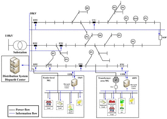
Figure 1.
System Diagram of Distribution Network and MGs.
The operation of distribution–microgrid systems is carried out under the coordinated interaction of day-ahead and intra-day scheduling, aiming to achieve an effective combination of global optimal scheduling and real-time dynamic adjustments. The day-ahead scheduling is primarily based on forecasts of the load demand and renewable generation for the following day, from which the overall operational strategy and resource allocation are formulated. In contrast, the intra-day scheduling is based on real-time load and generation data, dynamically adjusting the operational scheduling to respond to unpredictable short-term fluctuations and uncertainties. This coordinated operational model will fully leverage the advantages of distribution–microgrid systems in flexible regulation and resource optimization. On the one hand, the day-ahead scheduling provides macro-level guidance for stable system operation, optimizing the operation of distributed resources, reducing operational costs, and enhancing energy efficiency. On the other hand, the intraday dispatch schedules dynamically characterize the self-balancing capability of microgrids under uncertainty. It is worth noting that, as illustrated in Figure 1, the MGs discussed in this study operate at average voltage levels of 10 kV or 400 V.
3.1. Day-Ahead Economically Optimal Dispatch Scheduling Model
In the following, DA denotes the day-ahead variable, and ID denotes the intraday variable.
- (1)
- Power balance constraints
- (2)
- Controllable unit constraints
- (3)
- Power constraints between MG and ULG
- (4)
- Objective function
3.2. Intraday Model Considering Interactive Power Deviation
Unlike transmission–distribution network models, the controllable units in distribution-microgrid systems do not possess reserve capacity. Instead, they are limited to a small degree of flexibility for adjustment, based solely on the day-ahead scheduling.
- (1)
- Power balance constraints
- (2)
- Controllable unit constraints
Here, and represent the start time and end time for intra-day UFR analysis, respectively. Equation (13) ensures that the output of controllable units satisfies the ramping constraints between adjacent time periods within the intra-day UFR analysis.
- (3)
- Power constraints between MG and ULG
Here, represents the allowable IPDF. Equation (14) defines the range of allowable deviation.
Practically, most MGs are constructed as retrofits to existing distribution infrastructure, with their interconnection power typically designed to fully cover internal loads. Nevertheless, the increasing renewable energy penetration exacerbates source–load mismatch within MGs. Sole reliance on ULG to absorb such fluctuations poses significant risks to system security and stability. To address this limitation, this work intentionally permits controllable power exchange deviations between MGs and ULG. This paradigm shift aims to alleviate regulation pressure on transmission networks while systematically enhancing the renewable energy hosting capacity of integrated power systems.
- (4)
- Flexible load constraints
Here, and represent the upper and lower bounds of the flexible load output, respectively. denotes the time period for the intra-day UFR analysis. Equation (15) indicates that the flexible load has no impact on the load during the UFR analysis period. Equation (16) represents the output range of the flexible load.
We organize the above intra-day model inequalities into the following compact form:
Here, represents the set of linear inequality constraints formed by the MG’s intra-day variables, including renewable energy, load, controllable units, and the interaction power with the ULG. denotes the day-ahead scheduling, . is the row vector representing the output of controllable units in the day-ahead scheduling during the time period . is the row vector representing the interaction power output between the MG and the ULG in the day-ahead scheduling during period . represents the intra-day adjustable resources of the MG, . is the row vector representing the allowable deviation in the interaction power between the MG and the ULG at each moment during the intra-day UFR analysis period . is the row vector representing the output of controllable units at each moment during the intra-day UFR analysis period . is the row vector representing the output of flexible loads at each moment during the intra-day UFR analysis period . denotes the forecasted renewable generation. represents the fluctuation of renewable energy. In this paper, depending on the MG being evaluated, this fluctuation can refer to PV units, wind turbine units, or even the sum of both. represents the right-hand side of the constraints. are the corresponding constant matrices.
4. Outer Approximation Cutting Method for UFR
To obtain the UFR, specifically the maximum acceptable fluctuation range of renewable energy, this paper employs an OAC method. Firstly, is projected onto a low-dimensional space that is only related to , as shown in Equation (18).
For any point in the low-dimensional space , there exists a corresponding intra-day adjustment that satisfies Equation (19).
Here represents the set of all intraday flexible resource adjustment capabilities.
Definition 1.
The uncertainty feasible region is defined as set , satisfying and .
When the day-ahead scheduling is determined, Equation (17) defines a high-dimensional convex polytope composed of intra-day adjustable resource variables and renewable energy fluctuation variables, given that all constraints are linear. Equation (18) represents the projection of this high-dimensional convex polytope onto the direction of , resulting in another convex polytope, expressed as:
The problem of feasible region analysis essentially involves solving for and in Equation (20), as these contain the boundary information of the UFR. To acquire and , we introduce non-negative slack variables and , leading to the following optimization problem (21).
Here, and represent the measures taken by the MG in emergency situations.
If the optimization result of Equation (21) is positive, it indicates that the intra-day adjustable flexible resource is unable to fully mitigate the renewable energy fluctuation at that time and emergency measures must be applied by the MG control center. Conversely, if the optimization result of Equation (21) is zero, it suggests that at least one set of intra-day adjustable flexible resources can successfully mitigate the renewable energy fluctuation , eliminating the need for emergency measures. Given that the day-ahead scheduling is already determined and the renewable energy forecast is known, we introduce for simplification, which transforms Equation (21) into the following form:
Furthermore, when a sufficiently large initial space for the UFR is given, satisfying , the optimization problem can be transformed into determining whether the most critical point within the given initial space satisfies the MG constraints. Based on the principles of robust optimization, this can be expressed as problem (23):
Since all constraints are linear, the inner minimization problem can be transformed into its dual problem for analysis based on the weak duality theorem, resulting in problem (24).
In this formulation, represents the dual variable, while and are the boundary parameters of the given initial space .
When the most critical point in the given space satisfies the MG constraints, the optimization result of Equation (23) equals zero. According to the weak duality property, the maximum value of Equation (24) is less than or equal to the minimum value of the original problem (23), and the following inequality holds:
Equation (25) represents the constraints satisfied in the dual space when the most critical scenarios of the original problem comply with the MG constraints. In the optimization problem described by Equation (23), the most critical scenarios typically occur at the vertices of the polytope. According to duality theory, when the original problem takes a vertex solution, the dual problem also reaches its vertex. This implies that the search for boundary parameters and in the original problem is transformed into a vertex search in the dual problem.
For the initial space , it is theoretically sufficient to make it large enough to meet the requirements. However, this does not hold true in practical scenarios. Research has shown that the choice of the initial space significantly affects both the accuracy and efficiency of the feasible region analysis method proposed in this paper. The initial space can be determined through the following optimization problem:
Here, represents the matrix formed by the given search directions, and corresponds to the optimization result of Equation (26).
Umbrella constraints refer to the minimal set of constraints that preserve the optimal solution of the original optimization problem. During the optimization process, it is observed that many constraints are inactive. The optimization problem (27) is designed to find whether the -th constraint in the original problem qualifies as an umbrella constraint. In this study, the dimensionality of dual variables equals the number of MG constraints. By eliminating redundant constraints, the dimensionality of the dual variables is reduced, thereby decreasing computational complexity.
Here, represents the slack variable for identifying umbrella constraints, while denotes the corresponding -th row.
At this stage, the initial space required for model analysis has been obtained, and the umbrella constraints within the model have been identified. However, Equation (24) cannot yet be directly solved using a linear programming solver due to the nonlinearity of its objective function. Therefore, further reformulation is required, resulting in problem (28):
Here, represents the dual variable of the initial space constraints.
When the inner optimization problem reaches its optimal solution, the constraints satisfy the constraint qualifications, and its KKT conditions can be expressed as follows:
To eliminate the nonlinear constraints in Equation (29), the big-M method is applied to transform into the following constraints (30):
Here, M is a sufficiently large constant, and is a binary variable used to decouple the nonlinear constraints. So far, the model is obtained as follows:
Equation (31) can be solved using commercial software, and its solution determines whether the most critical point in the current space lies within the feasible region. The algorithm flowchart Figure 2 is as follows:
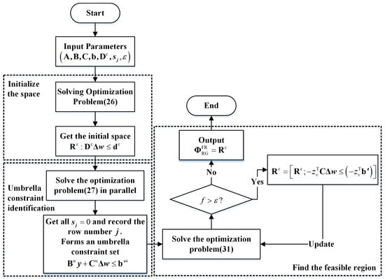
Figure 2.
Flowchart of outside approximation method to solve the feasible region.
5. Results
Taking a typical Transformer area MG as an example, it includes five controllable units, specifically micro gas turbine units, with their parameters listed in Table 1. The intra-day load curve, renewable generation forecast curve, and time-of-use electricity price are illustrated in Figure 3. The blue curve represents the time-of-use electricity price corresponding to the right y-axis, while the remaining curves correspond to the left y-axis. The day-ahead scheduling period is set as = 24, with a time resolution of = 1. For better visualization, the intra-day UFR analysis is conducted over a period of , with selected at 14:00, a time characterized by high renewable energy generation.

Table 1.
Controllable generators’ parameters.
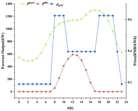
Figure 3.
Day-ahead parameters’ information.
The program is developed in MATLAB R2023b using YALMIP, running on a system with a 2.60 GHz processor and 16 GB of RAM. The proposed method is solved using IBM ILOG CPLEX 12.10 [27].
Based on the above data, the day-ahead optimal economic scheduling problem is solved to obtain the day-ahead scheduling. The dark blue curve in Figure 4 represents the interaction power between the MG and the ULG, corresponding to the right y-axis, while the remaining curves represent the output of the controllable units, corresponding to the left y-axis.
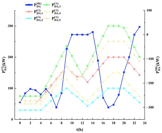
Figure 4.
Day-ahead dispatch scheduling.
By inputting the day-ahead scheduling and intra-day parameters into the model, and setting the allowable IPDF , the model is solved step by step to obtain the following results. Figure 5a shows the initial space determined by the given search directions, which contains many fluctuation points of renewable energy that do not satisfy the MG constraints. Figure 5b represents the obtained UFR, where the yellow area and its boundary indicate that, within the next three consecutive time periods, no emergency measures need to be applied by the MG. Instead, MG’s own flexible resources can adjust to meet all security constraints without affecting the day-ahead scheduling in subsequent periods. Figure 5c combines both, showing the result of their integration.
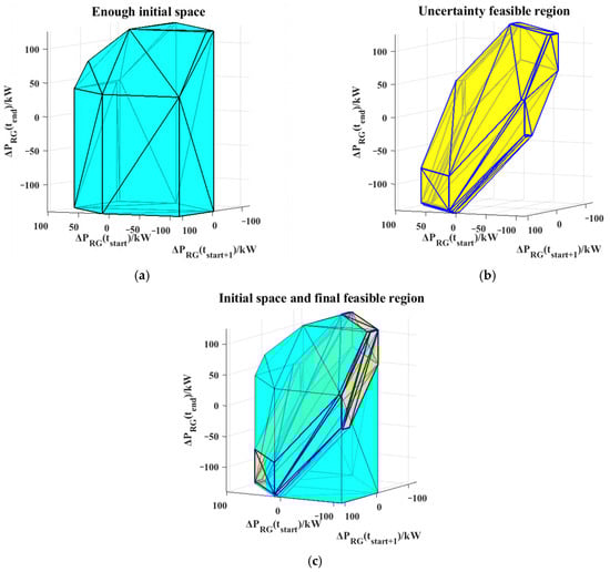
Figure 5.
Schematic Diagram of Initial Space and Feasible Region (a) Initial space; (b) Feasible region (lamda = 0.1); (c) Initial space and final feasible region.
As can be observed, due to the various constraints of the intra-day MG, including coupling constraints of controllable units across time periods and flexible load constraints, the initial space is progressively cut, with feasible cuts acting as cutting planes (instead of the traditional approach of searching for points or lines), thereby improving computational efficiency.
Next, we vary the allowable IPDF, setting it to 0.01, 0.1, and 0.2, respectively, and obtain the following figure. As shown in Figure 6, it can be observed that the range of UFR expands as the allowable IPDF increases. Although the geometries of feasible regions retain similarity, the cutting planes may vary significantly.
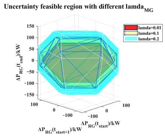
Figure 6.
UFR with different IPDFs.
The volume of the feasible region in three-dimensional space is used as an indicator to evaluate the size of the feasible region considering dispatch deviations in distribution–microgrid coordination. Taking as the reference, the volumes of the feasible region under different allowable IPDFs are as follows. As shown in Figure 7, the allowable IPDF significantly impacts the volume of the feasible region. Larger allowable deviations result in a larger feasible region, which aligns with practical expectations.
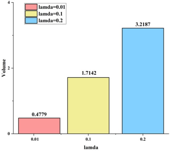
Figure 7.
Feasible region volumes for different IPDFs.
This indicates that when the interaction power between the MG and the ULG is permitted to deviate from the day-ahead scheduling, it effectively serves as an adjustable resource, like controllable units. As the amount of adjustable resources increases, the feasible region expands accordingly. As shown in Figure 8, we have quantified two main advantages of the research method proposed in this paper. In Figure 8a, adopting umbrella constraint identification accelerates the computational speed, and this acceleration becomes more pronounced as the system scale increases. In Figure 8b, when considering the deviation between the MG and the ULG, the volume of the MG’s UFR is significantly enlarged compared to when this deviation is not considered. This can be attributed to the significant benefits arising from the integration of enhanced flexibility resources in MGs.
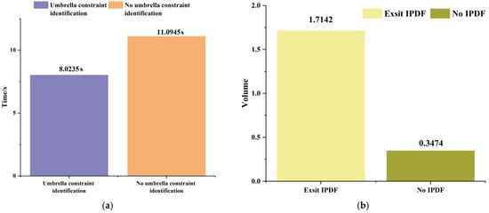
Figure 8.
The advantages of the proposed method; (a) Comparison of identification with and without umbrella constraints; (b) Comparison of whether IPDF between the MG and ULG is permitted.
6. Conclusions
This paper proposes an OAC method for UFR analysis. By utilizing umbrella constraint identification, redundant constraints in the model are eliminated, significantly improving the solution efficiency. The interaction power between the MG and the ULG is considered to allow deviations, treating these deviations as intra-day adjustable resources, thereby expanding the scope of the UFR. Using umbrella constraint identification and duality theory, the proposed method successfully characterizes the UFR. However, some limitations remain. The strong duality assumption depends on the linearity of the model, and nonlinear constraints from components such as energy storage systems are not considered. Future work will focus on incorporating energy storage into the model by removing discretization and adopting a continuous modeling approach.
Author Contributions
Conceptualization, J.Z. and P.L.; methodology, P.L.; software, X.J.; validation, P.L., X.J. and H.D.; formal analysis, P.W.; investigation, P.W.; resources, X.C.; data curation, X.C.; writing—original draft preparation, H.D.; writing—review and editing, H.D.; visualization, P.L.; supervision, J.Z.; funding acquisition, H.D. All authors have read and agreed to the published version of the manuscript.
Funding
This research was funded by the Science and Technology Project of State Grid Jiangsu Electric Power Co., Ltd. (Grant no. J2024137).
Conflicts of Interest
Author Hao Dong, Xiang Jiang, Xu Chen, and Puyan Wang were employed by the company Rugao Power Supply Company. The remaining authors declare that the research was conducted in the absence of any commercial or financial relationships that could be construed as a potential conflict of interest.
Abbreviations
The following abbreviations are used in this manuscript:
| MG | Microgrid |
| UFR | Uncertainty feasible region |
| OAC | Outer approximation cutting |
| ULG | Upper-level grid |
| IPDF | Interactive power deviation factor |
| PV | Photovoltaic |
References
- Liang, X. Emerging power quality challenges due to integration of renewable energy sources. IEEE Trans. Ind. Appl. 2016, 53, 855–866. [Google Scholar] [CrossRef]
- Zheng, Z.; Shafique, M.; Luo, X.; Wang, S. A systematic review towards integrative energy management of smart grids and urban energy systems. Renew. Sustain. Energy Rev. 2024, 189, 114023. [Google Scholar] [CrossRef]
- Tsikalakis, A.G.; Hatziargyriou, N.D. Centralized Control for Optimizing Microgrids Operation. IEEE Trans. Energy Convers. 2008, 23, 241–248. [Google Scholar] [CrossRef]
- Lasseter, R.H. MicroGrids. In Proceedings of the 2002 IEEE Power Engineering Society Winter Meeting, Conference Proceedings, New York, NY, USA, 27–31 January 2002. [Google Scholar]
- Dashtaki, A.A.; Hakimi, S.M.; Hasankhani, A.; Derakhshani, G.; Abdi, B. Optimal management algorithm of microgrid connected to the distribution network considering renewable energy system uncertainties. Int. J. Energy Syst. 2023, 145, 108633. [Google Scholar] [CrossRef]
- Li, A.; Peng, J.; Fan, L. Decentralized Optimal Operations of Power Distribution System with Networked Microgrids. In Proceedings of the 2023 IEEE Kansas Power and Energy Conference (KPEC), Manhattan, KS, USA, 27–28 April 2023. [Google Scholar]
- De la Torre, S.; Aguado, J.; Sauma, E. Optimal scheduling of ancillary services provided by an electric vehicle aggregator. Energy 2023, 265, 126147. [Google Scholar] [CrossRef]
- Majzoobi, A.; Khodaei, A. Application of microgrids in providing ancillary services to the utility grid. Energy 2017, 123, 555–563. [Google Scholar] [CrossRef]
- Jiang, T.; Zhang, R.; Li, X.; Chen, H.; Li, G. Integrated energy system security region: Concepts, methods, and implementations. Appl. Energy 2021, 283, 116124. [Google Scholar] [CrossRef]
- Li, X.; Tian, G.; Shi, Q.; Jiang, T.; Li, F.; Jia, H. Security region of natural gas network in electricity-gas integrated energy system. Int. J. Energy Syst. 2020, 117, 105601. [Google Scholar] [CrossRef]
- Hui, H.; Bao, M.; Ding, Y.; Song, Y. Exploring the integrated flexible region of distributed multi-energy systems with process. Industry. Appl. Energy 2022, 311, 118590. [Google Scholar] [CrossRef]
- Li, L.; Lin, W.; Yang, Z.; Yu, J.; Xia, S.; Wang, Y. Characterizing a tie-line transfer capacity region considering time coupling in day-ahead multi-period dispatch. Power Syst. Prot. Control 2020, 48, 64–72. [Google Scholar]
- Zhang, L.; Yang, G.; Wang, Y.; Li, L.; Lin, W.; Yang, Z.; Han, S. Determination of the DC tie-line transfer capacity region of the interconnected power grid: A multi-parametric programming approach. Proc. CSEE 2019, 39, 5763–5771+5904. [Google Scholar]
- Lin, W.; Yang, Z.; Yu, J.; Jin, L.; Li, W. Tie-line power transmission region in a hybrid grid: Fast characterization and expansion strategy. IEEE Trans. Power Syst. 2019, 35, 2222–2231. [Google Scholar] [CrossRef]
- Liu, Y.; Wu, L.; Li, J. A fast LP-based approach for robust dynamic economic dispatch problem: A feasible region projection method. IEEE Trans. Power Syst. 2020, 35, 4116–4119. [Google Scholar] [CrossRef]
- Qiu, H.; Li, Z.; Gao, H.; Nguyen, H.D.; Veerasamy, V.; Gooi, H.B. A Projection and Decomposition Approach for Multi-Agent Coordinated Scheduling in Power Systems. J. Mod. Power Syst. Clean Energy 2024, 12, 991–996. [Google Scholar] [CrossRef]
- Wen, Y.; Hu, Z.; You, S.; Duan, X. Aggregate feasible region of DERs: Exact formulation and approximate models. IEEE Trans. Smart Grid 2022, 13, 4405–4423. [Google Scholar] [CrossRef]
- Yi, Z.; Xu, Y.; Gu, W.; Yang, L.; Sun, H. Aggregate operation model for numerous small-capacity distributed energy resources considering uncertainty. IEEE Trans. Smart Grid 2021, 12, 4208–4224. [Google Scholar] [CrossRef]
- Zhang, M.; Xu, Y.; Shi, X.; Guo, Q. A fast polytope-based approach for aggregating large-scale electric vehicles in the joint market under uncertainty. IEEE Trans. Smart Grid 2023, 15, 701–713. [Google Scholar] [CrossRef]
- Müller, F.L.; Szabó, J.; Sundström, O.; Lygeros, J. Aggregation and disaggregation of energetic flexibility from distributed energy resources. IEEE Trans. Smart Grid 2017, 10, 1205–1214. [Google Scholar] [CrossRef]
- Zhang, H.; Cao, L. Research on demand side resource feasible region aggregation based on improved Zonotope. Power Demand Side Manag. 2024, 26, 1–7. [Google Scholar]
- Weibel, C. Minkowski Sums of Polytopes: Combinatorics and Computation. Ph.D.Dissertation, EPFL, Lausanne, Switzerland, 2007. [Google Scholar]
- Jiang, X.; Zhou, Y.; Ming, W.; Wu, J. Feasible operation region of an electricity distribution network. Appl. Energy 2023, 331, 120419. [Google Scholar] [CrossRef]
- Wang, Z.-Y.; Chiang, H.-D. On the nonconvex feasible region of optimal power flow: Theory, degree, and impacts. Int. J. Energy Syst. 2024, 161, 110167. [Google Scholar] [CrossRef]
- Zhang, T.; Wang, J.; Wang, H.; Jin, R.; Li, G.; Zhou, M. On the coordination of transmission-distribution grids: A dynamic feasible region method. IEEE Trans. Power Syst. 2022, 38, 1857–1868. [Google Scholar] [CrossRef]
- Kuznetsova, E.; Li, Y.-F.; Ruiz, C.; Zio, E. An integrated framework of agent-based modelling and robust optimization for microgrid energy management. Appl. Energy 2014, 129, 70–88. [Google Scholar] [CrossRef]
- Lofberg, J. YALMIP: A toolbox for modeling and optimization in MATLAB. In Proceedings of the 2004 IEEE International Conference on Robotics and Automation, Taipei, Taiwan, 2–4 September 2004. [Google Scholar]
Disclaimer/Publisher’s Note: The statements, opinions and data contained in all publications are solely those of the individual author(s) and contributor(s) and not of MDPI and/or the editor(s). MDPI and/or the editor(s) disclaim responsibility for any injury to people or property resulting from any ideas, methods, instructions or products referred to in the content. |
© 2025 by the authors. Licensee MDPI, Basel, Switzerland. This article is an open access article distributed under the terms and conditions of the Creative Commons Attribution (CC BY) license (https://creativecommons.org/licenses/by/4.0/).