Computing Idle Times in Fuzzy Flexible Job Shop Scheduling

Abstract

The flexible job shop scheduling problem is relevant in many different areas. However, the usual deterministic approach sees its usefulness limited, as uncertainty plays a paramount role in real-world processes. Considering processing times in the form of fuzzy numbers is a computationally affordable way to model uncertainty that enhances the applicability of obtained solutions. Unfortunately, fuzzy processing times add an extra layer of complexity to otherwise straightforward operations. For example, in energy-aware environments, measuring the idle times of resources is of the utmost importance, but it goes from a trivial calculation in the deterministic setting to a critical modelling decision in fuzzy scenarios, where different approaches are possible. In this paper, we analyse the drawbacks of the existing translation of the deterministic approach to a fuzzy context and propose two alternative ways of computing the idle times in a schedule. We show that, unlike in the deterministic setting, the different definitions are not equivalent when fuzzy processing times are considered, and results are directly affected, depending on which one is used. We conclude that the new ways of computing idle times under uncertainty provide more reliable values and, hence, better schedules.

1. Introduction

Scheduling is concerned with distributing and planning the execution of multiple tasks on a limited set of resources under different constraints, usually with the goal of optimising some objectives [1,2]. This kind of problem has multiple applications not only in industry and logistics but also in areas such as healthcare, education, or cloud computing [3,4,5,6,7].

The problems in the family known as job shop scheduling are especially significant because they can be used to model many real-world situations [8]. In a job shop, tasks or operations are part of jobs, so operations in a job must be executed in a given order. In the flexible variant, operations can be executed with different resources, so a resource-allocation problem arises in addition to the problem of sequencing operations belonging to different jobs within each resource [9,10]. In addition to presenting a challenge due to its complexity, the flexible job shop problem attracts special attention due to its relevance in modern industrial problems [11,12].

The majority of the research devoted to scheduling assumes that all parameter values are deterministic and well known in advance. However, in real life, it is often the case that some factors, e.g., processing times, are subject to variability due to machine or human influences. This source of uncertainty should not be dismissed; instead, the proper management of the non-deterministic elements of the scheduling process is especially important in Industry 5.0 solutions [13]. In particular, uncertainty in operation processing times can be addressed with stochastic models or, alternatively, using fuzzy numbers. Following the pioneering works [14,15] fuzzy sets and fuzzy numbers have been amply used in scheduling [16,17,18,19]. The reviews [20,21] provide many examples where fuzzy numbers have been successfully applied to shop scheduling problems. In the particular case of the fuzzy flexible job shop scheduling problem, some works consider traditional production-related objectives, for instance, weighted tardiness and earliness [22], makespan [23], or makespan and total workload [24], while others focus on energy efficiency [25,26]. We can also find multiobjective proposals that combine the optimisation of energy consumption together with more traditional objectives, such as makespan or deadline satisfaction [27,28,29,30]. A survey of solving methods can be found in [31].

Associated with a schedule are the concepts of idle and waiting times. Idle time is the time spent with the resources waiting to process operations, while the waiting time, its counterpart from the job point of view, is the time spent by jobs waiting for the resources to become available. Idle and waiting times can be of interest for several reasons: they can be part of a constraint, they may constitute an objective in themselves, they may be a component of some other performance objective function, or it may be necessary to compute them as part of a solution method.

Idle and waiting times act as hard constraints when no-wait or no-idle schedules are required. In other cases, a strict no-wait or no-idle constraint might be relaxed and, instead, waiting or idle times need to be kept as small as possible for technological reasons. For example, in food industries, an excessive waiting time after an operation might cause the produced goods to be spoilt and unusable for later operations, or in chemical industries, it can be the case that no waiting time can be allowed between warming and manufacturing operations in the same job. Likewise, it may be undesirable or simply not allowed to have idle resources, for instance, when machines require consumable products, such as paints or powders, that become unusable if the machine stays idle for too long (e.g., paint becomes dried or powder oxidises), or in the steel industry, where furnaces must be kept at a high temperature at all times, regardless of whether they are active or idle. More generally, idle times can be relevant indicators of the efficiency of production systems, especially in those where expensive resources are part of the considered production layout since idle times are directly related to resource utilisation. Also, minimising the total core idle time (i.e., the idle time within the system) is strongly aligned with minimising the makespan, a classical objective in scheduling. Beyond manufacturing, in service environments where the resources are human workers (e.g., in healthcare), it may be desirable to minimise idle times not only to reduce costs and gain efficiency but also to maximise workers’ satisfaction [32,33,34].

Idle times have garnered increasing attention with the growth of energy-aware or green scheduling. According to [35], studies on energy-efficient scheduling are classified into four groups based on energy-saving methods. The first is to reduce unnecessary idle time: it is estimated that, in actual manufacturing processes, machine tools stay idle most of the time and consume about 80% of energy while being in this idle state; in consequence, over 30% of the articles reviewed in [36] consider idle energy consumption as part of the objective function to be minimised. The second approach is to directly turn off the resources when the idle time is long enough and the energy savings compensate for the cost of turning on/off. The third approach is to adjust the machine speed when energy consumption depends on it. Finally, the fourth one is to favour off-peak production: given that, in peak time, electricity costs (and associated pollution) are high, scheduling part of the production at a non-peak time can save a significant amount of electricity cost and mitigate pollution.

We find in the literature many recent examples of green scheduling (many flexible job shop problems) where idle times play an important part. In [35], they consider an energy-efficient flexible job shop under time-of-use pricing and scheduled downtime. With prices of electricity varying over discrete time intervals, the key is to take advantage of idle times and shift the inevitable idle time to peak periods and the production to off-peak periods in order to minimise the energy cost. The flexible job shop problem is also addressed in [37,38]. In the former, the objective is to minimise the total energy consumption by adopting an on/off strategy that takes into account idle times. In the latter, energy consumption is composed of processing energy consumption, idle energy consumption, setup energy consumption, and common energy consumption. A multiobjective dynamic version of the flexible job shop scheduling problem minimising both energy and completion time is tackled in [39] through idle machine time arrangement and machine speed level selection. Inspired by real-world problems, in [40], they present an approach to minimising idle energy consumption and apply it to a heat-intensive process employing a steel-hardening furnace, which requires a high power input to reach and maintain the specific operating temperature, so a considerable amount of energy is consumed even during the periods when no material is being processed. Ref. [41] addresses scheduling in virtual network functions, modelled as a job shop problem, with the goal of simultaneously minimising the makespan and the idle energy loss. In [42] we find another multiobjective scheduling problem, here applied to bakery production, taking into account the reduction in oven idle times as a means of reducing energy consumption. The results show that, by penalising the best makespan by a marginal amount, alternative optimal solutions obtain a considerable reduction in oven idle time by up to 61%, resulting in a strategy that allows small and medium-sized bakeries to lower production costs and reduce ${\mathrm{CO}}_2$ emissions.

Clearly, to enhance its scope of application and come closer to solving real-world problems, fuzzy scheduling also needs to handle and take into account idle times. However, computing idle times between operations in a resource or the total time a resource is idle is far from trivial in the fuzzy setting since it is not possible to directly extend the equations and techniques from the deterministic framework. This may be the reason why few attempts have been made in this direction, with a few exceptions. Idle times between operations are used to calculate the idle energy consumption in a fuzzy job shop in [43], while multiobjective versions of this problem are tackled in [44,45]. In the first case, idle gaps are used to right-shift operations with the goal of reducing the energy consumption of a given schedule, and in the second case, MIP post-processing makes use of these idle times to also improve the energy cost of a schedule.

Below, we will address the fuzzy flexible job shop problem. We will illustrate the difficulties inherent to computing idle times in the fuzzy framework. We will propose two different ways of computing the idle times between operations in a resource, as well as a third way of directly computing the total idle time in a resource. We will argue that, although, in the deterministic setting these three approaches are equivalent and yield the same value for the total core idle time in a schedule, that is not the case under uncertainty. We will finally conduct an experimental study to empirically evaluate the three proposals for computing idle times in fuzzy schedules.

2. The Fuzzy Flexible Job Shop Problem

The flexible job shop scheduling problem consists in scheduling a set $\mathbf{O}$ of operations (also called tasks) in a set $\mathbf{R}$ of m resources (also called machines) subject to a set of constraints. Operations are organised in a set, $\mathbf{J}$, of n jobs, so operations within a job must be sequentially scheduled. Given an operation, $o\in \mathbf{O}$, $\chi \left(o\right)$ will denote the job in $\mathbf{J}$ that this operation belongs to, and $\eta \left(o\right)$ will denote the relative position of o in the job, $\chi \left(o\right)$. Each operation, $o\in \mathbf{O}$, can only be processed in resources from a given subset, $\mathbf{R}\left(o\right)\subseteq \mathbf{R}$, with a processing time, $p(o,r)$, which is dependent on the resource, $r\in \mathbf{R}\left(o\right)$, where it is executed. Furthermore, the following statements are assumed:

• All jobs and resources are available at the first instant of time.
• Preemption is not allowed; i.e., each operation must be completed without interruption once started.
• Machines cannot perform more than one operation at a time.
• Transportation times between resources and setup times are negligible.
• Operations are assumed to be successfully completed after the first attempt; the scrap rate is zero.
• The available capacity of resources is known; there are no stoppages, breakdowns, etc.
• Buffers with infinite capacity are available for all resources.

Under this problem formulation, the idle time is the time spent by a resource waiting for an operation to process it. The total idle time in a resource can usually be decomposed into front, back, and core idle times. The front idle time is the time a resource waits before starting the first operation (while other resources are already working), the back idle time is the time between the instant when a resource completes its last operation and the instant the last resource finishes working, and the core idle time refers to the time a resource is idle between operations, that is, once it has finished processing one operation and is waiting for the next operation to start being processed.

The objective of this paper is to minimise the total core idle time (that is, the sum of core idle times for all resources) in the fuzzy flexible job shop. In the following subsections, we will describe how to work with fuzzy processing times and how they affect idle time calculations. The notation used throughout the paper is summarised in

Table 1. Table of symbols.

Symbol	Description
$\mathbf{O}$	set of operations
$\mathbf{R}$	set of resources
m	number of resources
$\mathbf{J}$	set of jobs
n	number of jobs
$\mathbf{R}\left(o\right)$	subset of resources in which operation o can be executed
$\chi \left(o\right)$	job to which operation o belongs to
$\eta \left(o\right)$	position in which operation o has to be executed relative to its job
$p(o,r)$	processing time of operation o in the resource r
${\mathit{\tau }}_{\varphi }$	resource assignments in solution $\varphi$
${\mathbf{s}}_{\varphi }$	operation starting times in solution $\varphi$
${\tau }_{\varphi }\left(o\right)$	resource assigned to operation o in solution $\varphi$
$s_{\varphi }\left(o\right)$	position of operation o in ${\tau }_{\varphi }\left(o\right)$
$p_{\varphi }\left(o\right)$	processing time of operation o in solution $\varphi$. Equivalent to $p(o,{\tau }_{\varphi }\left(o\right))$
$c_{\varphi }\left(o\right)$	completion time of operation o in solution $\varphi$
$JP\left(o\right)$	job predecessor of operation o
$JS\left(o\right)$	job successor of operation o
${RP}_{\varphi }\left(o\right)$	resource predecessor of operation o in solution $\varphi$
${RS}_{\varphi }\left(o\right)$	resource successor of operation o in solution $\varphi$
${\alpha }_{\varphi }\left(r\right)$	first operation scheduled in resource r in solution $\varphi$
${\omega }_{\varphi }\left(r\right)$	last operation scheduled in resource r in solution $\varphi$
$\widehat{\square }$	all notations with a hat represent that the number is TFN
${\square }^i$	refers to the i-th component of a fuzzy number
${\square }^N$	refers to a measure computed using the Naive approach
${\square }^K$	refers to a measure computed using the schedule Knowledge approach
${\square }^C$	refers to a measure computed using the Coarse approach
$I_{\varphi }\left(o\right)$	idle time of an operation in $\varphi$
$CI{T}_{\varphi }\left(r\right)$	core idle time of a resource in $\varphi$
$TCI{T}_{\varphi }$	total core idle time of $\varphi$
$\mathit{\rho }$	a crisp scenario
$f_{\varphi }^{\mathit{\rho }}$	value of the objective function f under the crisp scenario $\mathit{\rho }$ in solution $\varphi$
$\mathbb{E}\left[\widehat{a}\right]$	expected value of $\widehat{a}$
$S\left(\widehat{a}\right)$	spread of $\widehat{a}$
$MVP\left(\widehat{a}\right)$	modal value position of $\widehat{a}$
$RDEV(\varphi ,\mathit{\rho })$	relative distance to the expected value of $\varphi$ with respect to the crisp scenario $\mathit{\rho }$
$UU(\varphi ,\mathbf{S})$	used uncertainty of solution $\varphi$ in the set of possible scenarios $\mathbf{S}$

.

2.1. Fuzzy Processing Times

It is fairly common in the literature to model uncertain processing times as triangular fuzzy numbers (TFNs), defined by an interval, $[a^1,a^3]$, of possible values (its support) and a modal value, $a^2$ [16]. A TFN can be represented as a triplet, $\widehat{a}=(a^1,a^2,a^3)$, so its membership function is given by the following:

$${\mu }_{\widehat{a}}\left(x\right)=\left\{\begin{array}{cc}{\displaystyle \frac{x-a^1}{a^2-a^1}}\hfill & a^1\le x\le a^2\hfill \\ {\displaystyle \frac{x-a^3}{a^2-a^3}}\hfill & a^2\le x\le a^3\hfill \\ 0\hfill & \mathrm{otherwise}\hfill \end{array}\right.$$

(1)

Arithmetic operations on TFNs are defined based on the Extension Principle [46], so for two TFNs, $\widehat{a}$ and $\widehat{b}$, the sum is a TFN defined as follows:

$$\widehat{a}+\widehat{b}=(a^1+b^1,a^2+b^2,a^3+b^3),$$

(2)

And their difference is a TFN defined as follows:

$$\widehat{a}-\widehat{b}=(a^1-b^3,a^2-b^2,a^3-b^1).$$

(3)

At first, the resulting expression for the subtraction may seem counter-intuitive. However, notice that the smallest possible value that the uncertain variable, a, described by $\widehat{a}$, may take is $a^1$, while the greatest possible value for the uncertain variable, b, described by $\widehat{b}$, is $b^3$ and, hence, the smallest possible value for their difference is $a^1-b^3$. Analogously, the greatest possible value for the difference will be $a^3-b^1$. This results in support for the difference where the extreme values of the two involved TFNs can be said to be “crossed”. Interestingly enough, the same expressions for the sum and the difference are obtained if we reconstruct them via interval computation from the alpha-cuts [16,46]. A consequence of these definitions is that, in the set of TFNs, the difference is not necessarily the inverse of the sum, that is, $\widehat{a}\ne (\widehat{a}+\widehat{b})-\widehat{b}$. This is because underlying the definition (3) that results from the Extension Principle is the assumption that the uncertain variables a and b associated with $\widehat{a}$ and $\widehat{b}$ are non-interactive; i.e., they can take values in their support independently of each other. Therefore, when the TFNs $\widehat{a}$ and $\widehat{b}$ are linked, the resulting difference may be an “over-uncertain” or “pessimistic” quantity. This may prove to be an issue in certain applications; it is, for instance, the main difficulty in critical-path analysis and backpropagation in activity networks with fuzzy durations [16].

Unlike the cases of addition and subtraction, the set of TFNs is not closed under the extended maximum. For this reason, in fuzzy scheduling, it is usual to approximate the maximum of two TFNs via interpolation as follows:

$$max(\widehat{a},\widehat{b})\approx (max(a^1,b^1),max(a^2,b^2),max(a^3,b^3)).$$

(4)

The approximation always preserves the support and the modal value, and, if the result of the extended maximum is a TFN, it coincides with the approximated value (cf. [47]).

Given that the set of TFNs is not endowed with a natural total order, it is common practice to resort to some ranking method to make comparisons. A widely used one is that based on expected values. For a TFN, $\widehat{a}$, its expected value is as follows:

$$\mathbb{E}\left[\widehat{a}\right]={\displaystyle \frac{a^1+2a^2+a^3}{4}},$$

(5)

So, any two TFNs $\widehat{a}$ and $\widehat{b}$ can be compared as follows:

$$\widehat{a}{\le }_E\widehat{b}\mathrm{if}\mathrm{and}\mathrm{only}\mathrm{if}\mathbb{E}\left[\widehat{a}\right]\le \mathbb{E}\left[\widehat{b}\right].$$

(6)

Accordingly, we will write $\widehat{a}{<}_E\widehat{b}$ when $\mathbb{E}\left[\widehat{a}\right]<\mathbb{E}\left[\widehat{b}\right]$. The ranking induced via the expected value coincides with several other rankings from the literature; it is also related to classical interval comparisons via imprecise probabilities, and it has been empirically shown to result in more robust solutions when used in fuzzy scheduling [47,48].

In addition, we consider the following precedence relation between any pair of two TFNs, $\widehat{a}$ and $\widehat{b}$:

$$\widehat{a}⪯\widehat{b}\mathrm{if}{a}^i\le b^i\forall i\in \{1,2,3\},$$

(7)

with strong precedence, $\widehat{a}\preccurlyeq \widehat{b}$, if and only if $\widehat{a}⪯\widehat{b}\wedge \exists i\in \{1,2,3\}{a}^i<b^i$.

2.2. Fuzzy Schedules

A solution to the problem, commonly called a schedule and denoted as $\varphi =({\mathit{\tau }}_{\varphi },{\mathbf{s}}_{\varphi })$, consists of both a resource assignment, ${\mathit{\tau }}_{\varphi }$, and a starting time assignment, ${\mathbf{s}}_{\varphi }$, for all operations. This solution is feasible if and only if all precedence and capacity constraints hold. More formally, for an operation, $o\in \mathbf{O}$, let ${\tau }_{\varphi }\left(o\right)$ be the resource to which it is assigned in $\varphi$, and let $\widehat{s_{\varphi }}\left(o\right)$ and $\widehat{c_{\varphi }}\left(o\right)=\widehat{s_{\varphi }}\left(o\right)+\widehat{p}(o,{\tau }_{\varphi }\left(o\right))$ be, respectively, its starting and completion times in the solution $\varphi$. Then, precedence constraints hold for $\varphi$ if and only if, for any pair of operations, $o,u\in \mathbf{O}$,

$$\widehat{c_{\varphi }}\left(o\right)⪯\widehat{s_{\varphi }}\left(u\right)\mathrm{when}\chi \left(o\right)=\chi \left(u\right),\eta \left(o\right)<\eta \left(u\right)$$

(8)

and capacity constraints hold if and only if

$$\begin{array}{c}{\tau }_{\varphi }\left(o\right)\in \mathbf{R}\left(o\right)\end{array}$$

(9)

$$\begin{array}{c}\widehat{c_{\varphi }}\left(o\right)⪯\widehat{s_{\varphi }}\left(u\right)\vee \widehat{c_{\varphi }}\left(u\right)⪯\widehat{s_{\varphi }}\left(o\right)\mathrm{when}{\tau }_{\varphi }\left(o\right)={\tau }_{\varphi }\left(u\right).\end{array}$$

(10)

Notice that a feasible starting time assignment, ${\mathbf{s}}_{\varphi }$, induces an ordering for all the operations in the same resource. In the sequel, given a resource, $r\in \mathbf{R}$, let ${\alpha }_{\varphi }\left(r\right)$ denote the first operation to be processed in r according to schedule $\varphi$, and let ${\omega }_{\varphi }\left(r\right)$ be the last operation to be processed in r. Also, for an operation, $o\in \mathbf{O}$, let $\mathit{JP}\left(o\right)$ (resp. $\mathit{JS}\left(o\right)$) denote its immediate predecessor (resp. successor) in its job, ${\mathit{RP}}_{\varphi }\left(o\right)$ (resp. ${\mathit{RS}}_{\varphi }\left(o\right)$) its immediate predecessor (resp. successor) in its resource according to the ordering induced via $\varphi$, and $\widehat{p_{\varphi }}\left(o\right)=\widehat{p}(o,{\tau }_{\varphi }\left(o\right))$ the operation’s processing time in the resource to which it is assigned.

A feasible schedule is semi-active if no operation, o, can start earlier (in the sense that it can be assigned another starting time, ${\widehat{s}}^{\prime }\left(o\right)$, such that ${\widehat{s}}^{\prime }\left(o\right)\preccurlyeq \widehat{s_{\varphi }}\left(o\right)$) without changing the order of processing on any of the resources. In consequence, for a semi-active schedule, the starting time of any operation, o, is the earliest starting time of that operation according to the job and resource processing orders:

$$\widehat{s_{\varphi }}\left(o\right)=max\{\widehat{c_{\varphi }}\left(\mathit{JP}\left(o\right)\right),\widehat{c_{\varphi }}\left({\mathit{RP}}_{\varphi }\left(o\right)\right)\}$$

(11)

where $\widehat{c_{\varphi }}\left(\mathit{JP}\left(o\right)\right)$ (resp. $\widehat{c_{\varphi }}\left({\mathit{RP}}_{\varphi }\left(o\right)\right)$) is taken to be $(0,0,0)$ if $\eta \left(o\right)=min\left\{\eta \right(u):\chi (u)=\chi (o\left)\right\}$, that is, o is the first operation in its job (resp. o is the first operation in its resource, $o={\alpha }_{\varphi }\left({\tau }_{\varphi }\left(o\right)\right)$).

For so-called regular objective functions (those which are non-decreasing functions of the jobs’ completion times), optimal schedules are necessarily semi-active. Assuming semi-active schedules reduces the total number of feasible schedules from infinity to a finite (albeit possibly large) number, with each set of resource orderings providing a single semi-active schedule. For this reason, it is common in the scheduling literature to consider only semi-active schedules. Unless otherwise stated, this will also be assumed here.

2.3. Comparing Fuzzy Schedules

The quality of a schedule, $\varphi$, is usually measured in terms of a performance or cost function, $f_{\varphi }$, so the objective is to find a schedule that minimises f. When working with fuzzy durations, the cost of a fuzzy schedule, $\varphi$, becomes a TFN ${\widehat{f}}_{\varphi }$, representing the possible values that the cost, f, may take when $\varphi$ is executed.

When the performance of a schedule, $\varphi$, is given by a TFN ${\widehat{f}}_{\varphi }$, the expected value, $\mathbb{E}\left[{\widehat{f}}_{\varphi }\right]$, summarises the schedule’s performance in a single crisp value (which allows for comparisons between schedules in the absence of a natural order in the set of TFNs). The quality of a fuzzy schedule $\varphi$ can be further assessed using the measures proposed in [26]. These are concerned, first, with the level of uncertainty in the value ${\widehat{f}}_{\varphi }$ and, second, with the robustness and accuracy of the fuzzy number ${\widehat{f}}_{\varphi }$ as a predictor of the actual performance of the schedule when it is executed in a real scenario.

2.3.1. Measures Based on Fuzzy Values

Further insight into a schedule’s quality may be gained by considering, in addition to the expected value of fuzzy numbers, two additional features of a TFN $\widehat{a}$:

• The spread (S) of a TFN $\widehat{a}$, given by

  $$S\left(\widehat{a}\right)=a^3-a^1,$$

  (12)

  is a measure of the level of uncertainty in the TFN. Although uncertainty is unavoidable, a solution with a smaller spread in ${\widehat{f}}_{\varphi }$ should be preferred.
• The modal value position (MVP), defined as

  $$\mathit{MVP}\left(\widehat{a}\right)={\displaystyle \frac{(a^2-a^1)-(a^3-a^2)}{a^3-a^1}},$$

  (13)

  is a number in $[-1,1]$, which is negative when the TFN’s modal value $a^2$ is to the left of the support’s midpoint, positive when the modal value is to the right of the midpoint, and zero when the TFN is symmetric. It could somehow be seen as a measure of the skewness of the TFN. Values closer to 0 seem preferable in the sense that they are less biased to either optimistic or pessimistic values.

2.3.2. Measures Based on Possible Crisp Realisations

According to the semantics of fuzzy schedules proposed in [49], a fuzzy schedule, $\varphi$, is an a priori or predictive solution providing a possibility distribution (in the form of TFNs) for the starting times of all operations and, in consequence, for the values of the resulting performance function, f. When operations are actually executed according to the resource assignment and the ordering induced via the schedule, uncertainty is no longer present: for each operation, o, its executed processing time, $p_{\varphi }\left(o\right)$, is a crisp value in support of the fuzzy processing time ${\widehat{p}}_{\varphi }\left(o\right)$; i.e., it is a possible crisp realisation of the fuzzy processing time. The vector of executed processing times, $\mathit{\rho }$, where $\rho \left(o\right)=p_{\varphi }\left(o\right)$, is a vector of possible realisations of the fuzzy processing times, also called a possible scenario. In consequence, the performance $f_{\varphi }^{\mathit{\rho }}$ of the executed schedule is a crisp value in support of the fuzzy performance ${\widehat{f}}_{\varphi }$. Thus, the executed schedule can be seen as the a posteriori realisation of the fuzzy schedule $\varphi$.

Under these semantics, the quality of the a priori fuzzy schedule can be measured relative to its a posteriori performance in a possible scenario or, more generally, across a set of different possible scenarios. To this end, let $\mathbf{S}$ be a set of possible scenarios. We can define the following measures for $\varphi$:

• Relative distance to the expected value (RDEV) in a possible scenario:

  $$\mathit{RDEV}(\varphi ,\mathit{\rho })={\displaystyle \frac{f_{\varphi }^{\mathit{\rho }}-\mathbb{E}\left[{\widehat{f}}_{\varphi }\right]}{\mathbb{E}\left[{\widehat{f}}_{\varphi }\right]}}$$

  (14)
  If this value is negative, that is, the cost in the executed schedule is smaller than expected, it means that the a priori schedule objective function is pessimistic. On the contrary, if $\mathit{RDEV}$ is positive, the a priori schedule could be seen as optimistic. Overall, the smaller the absolute value of $\mathit{RDEV}$, the closer the predicted performance of the solution to the real performance once the schedule is executed.
• Used uncertainty (UU) in a set of possible scenarios:

  $$\mathit{UU}(\varphi ,\mathbf{S})={\displaystyle \frac{{max}_{\mathit{\rho }\in \mathbf{S}}{f}_{\varphi }^{\mathit{\rho }}-{min}_{\mathit{\rho }\in \mathbf{S}}{f}_{\varphi }^{\mathit{\rho }}}{f_{\varphi }^3-f_{\varphi }^1}}$$

  (15)
  This is a value in $[0,1]$ measuring the proportion of the support of the predicted fuzzy objective function ${\widehat{f}}_{\varphi }$ that is actually covered across the range of possible scenarios in $\mathbf{S}$. When $\mathbf{S}$ is representative enough of all the possible scenarios, a value of $\mathit{UU}$ close to 1 means that the range of values considered as possible by the TFN ${\widehat{f}}_{\varphi }$ is actually obtainable in real situations. On the other hand, small values of $\mathit{UU}$ would mean that the fuzzy schedule incorporates “artificial” uncertainty by considering possible values of f that are in fact never achieved, thus being less informative.

3. Idle Times with Fuzzy Durations

In a deterministic setting, given a schedule, $\varphi$, it is trivial to compute core idle time before an operation, o: it suffices to subtract the completion time of its immediate predecessor in the resource ${\mathit{RP}}_{\varphi }\left(o\right)$ from the starting time of o. Then, the core idle time for a resource r, ${CIT}_{\varphi }\left(r\right)$, is obtained by adding the core idle time for all the operations assigned to the resource. Equivalently, ${CIT}_{\varphi }\left(r\right)$ can be obtained as the difference between the time span since the resource starts processing the first operation until the last operation is finished and the total time spent by the resource executing operations. Finally, the total core idle time, ${TCIT}_{\varphi }$, is the sum of core idle times across all resources $r\in \mathbf{R}$.

Our goal will be to find a schedule minimising the total core idle time. However, extending these definitions to the fuzzy context is not trivial. The cause is the assumption of independence underlying the definition of the fuzzy subtraction, together with the fact that it is not the inverse of the sum (thus losing the equivalence between the two ways of defining the core idle time for a resource).

In the sequel, we propose three different ways of computing the core idle time of a resource, $r\in \mathbf{R}$, given a fuzzy schedule, $\varphi$, ${\widehat{CIT}}_{\varphi }\left(r\right)$. In the first two cases, we start by proposing a means to compute the core idle time, ${\widehat{I}}_{\varphi }\left(o\right)$, of every operation, o, scheduled in the resource, r, and we then obtain ${\widehat{CIT}}_{\varphi }\left(r\right)$ as the sum of core idle times across all operations executed in r. In the last case, we adopt a less granular approach and define ${\widehat{CIT}}_{\varphi }\left(r\right)$ directly as the time span between the starting of the first operation in the resource and the completion of the last operation in the same resource, minus the time spent by the resource processing its operations.

3.1. A Naive Approach

The most straightforward approach to computing the time a resource, r, is idle waiting for an operation, o, under a fuzzy schedule, $\varphi$, denoted as ${\widehat{I}}_{\varphi }\left(o\right)$, is to subtract the completion time of the operation’s immediate resource predecessor, $R{P}_{\varphi }\left(o\right)$, from the starting time of o. This is a direct translation of how the idle time can be computed in a deterministic setting, and it has been applied several times in the fuzzy scheduling literature [43,44,45]. Taking into account that negative values for idle times are impossible, this translates into the following definition:

$${\widehat{I}}_{\varphi }^N\left(o\right)=\left\{\begin{array}{cc}(0,0,0)\hfill & \mathrm{if}o={\alpha }_{\varphi }\left({\tau }_{\varphi }\left(o\right)\right),\hfill \\ max\{(0,0,0),{\widehat{s}}_{\varphi }\left(o\right)-{\widehat{c}}_{\varphi }\left(R{P}_{\varphi }\left(o\right)\right)\}\hfill & \mathrm{otherwise}.\hfill \end{array}\right.$$

(16)

That is, if o is the first operation to be processed in its resource $r={\tau }_{\varphi }\left(o\right)$, the idle time before o is null, and otherwise, it is the difference between the operation’s starting time and its predecessor’s completion time, discounting negative values (which we know are impossible). Then, the core idle time for resource r is given by the sum of idle time for the operations scheduled in r:

$${\widehat{CIT}}_{\varphi }^N\left(r\right)=\sum _{o\in \mathbf{O}:{\tau }_{\varphi }\left(o\right)=r}{\widehat{I}}_{\varphi }^N\left(o\right)$$

(17)

The problem with this straightforward extension of the deterministic definition is that, as mentioned in Section 2.1, the fuzzy subtraction assumes that the variables involved are non-interactive. Making such an assumption for two consecutive operations in a resource is at least naive and, in most cases, problematic. Indeed, in a feasible schedule, an operation, o, cannot start before its immediate processor is completed, so there is a clear dependence between ${\widehat{s}}_{\varphi }\left(o\right)$ and ${\widehat{c}}_{\varphi }\left(R{P}_{\varphi }\left(o\right)\right)$. This dependence is highly marked in the case of semi-active schedules, where ${\widehat{s}}_{\varphi }\left(o\right)$ is defined in terms of ${\widehat{c}}_{\varphi }\left(R{P}_{\varphi }\left(o\right)\right)$, as shown in Equation (11). 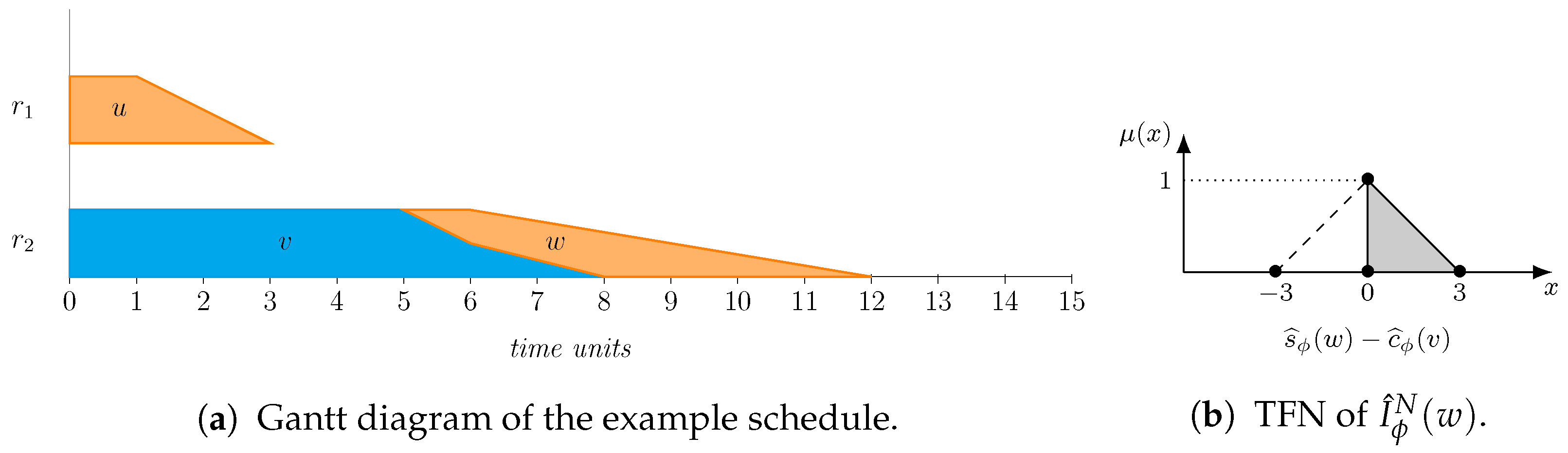As a result, computing the idle time for an operation, o, using (16) will most likely result in a quantity with added artificial uncertainty in the sense that many values in its support are actually unattainable. Let us illustrate this with an example:

Let u, v, and w be the only three operations in a schedule $\varphi$ where u, the job predecessor of w, is processed on its own in a resource, while v is the resource predecessor of w in a second resource. Let the processing times of these tasks be ${\widehat{p}}_{\varphi }\left(u\right)=(1,2,3)$, ${\widehat{p}}_{\varphi }\left(v\right)=(5,6,8)$, and ${\widehat{p}}_{\varphi }\left(w\right)=(1,3,4)$. Clearly, if u and v start at instant 0, their completion times are, respectively, $\widehat{c}\left(u\right)=(1,2,3)$ and $\widehat{c}\left(v\right)=(5,6,8)$. Hence, the completion time of u cannot affect the starting time of w, ${\widehat{s}}_{\varphi }\left(w\right)$, which, for any feasible schedule, must be such that $\widehat{c}\left(v\right)⪯\widehat{s}\left(w\right)$, with an equality for semi-active schedules, i.e., $\widehat{s}\left(w\right)=\widehat{c}\left(v\right)=(5,6,8)$. The Gantt chart of the schedule, adapted to TFNs, as proposed in [50], can be seen in Figure 1. Now, if we compute the difference, ${\widehat{s}}_{\varphi }\left(w\right)-{\widehat{c}}_{\varphi }\left(v\right)=(5-8,6-6,8-5)=(-3,0,3)$. This number is counterintuitive for two reasons. First, allowing for negative idle time values does not make any sense. This is solved by taking the maximum with, $(0,0,0)$; so, according to (16), the idle time for w is $I^N\left(w\right)=(0,0,3)$. We depict the resulting TFN in Figure 1b, where the dashed line represents the negative side that is removed, with the area under the membership function for $I^N\left(w\right)$ shaded in grey. The second reason is that common sense dictates that the idle time between two contiguous operations should be zero, as the absence of a gap between v and w in Figure 1 illustrates, but even after eliminating negative values, $I^N\left(w\right)$ considers as possible idle times as large as 3. The source of these issues is the wrong underlying assumption that $\widehat{s}\left(w\right)$ and $\widehat{c}\left(v\right)$ are independent; so, for instance, $s\left(w\right)$ could be 5 when $c\left(v\right)$ is 8 (even if we know this is impossible in a feasible schedule). That is, the independence assumption introduces artificial uncertainty in the resulting difference.

3.2. An Approach Incorporating Schedule Knowledge

If we consider again the previous example, the problem stems from the fact that ${\widehat{s}}_{\varphi }\left(w\right)$ and ${\widehat{c}}_{\varphi }\left(v\right)$ are linked variables. Indeed, the starting time of w is computed according to Equation (11); that is, ${\widehat{s}}_{\varphi }\left(w\right)=max\{{\widehat{c}}_{\varphi }\left(u\right),{\widehat{c}}_{\varphi }\left(v\right)\}$. Substituting in the difference component of the idle time (16),

$${\widehat{s}}_{\varphi }\left(w\right)-{\widehat{c}}_{\varphi }\left(v\right)=max\{{\widehat{c}}_{\varphi }\left(u\right),{\widehat{c}}_{\varphi }\left(v\right)\}-{\widehat{c}}_{\varphi }\left(v\right).$$

Now, given the way in which the difference and the maximum are defined in (3) and (4), we can rearrange the elements in this equation, so

$${\widehat{I}}_{\varphi }^N\left(w\right)=max\{(0,0,0),{\widehat{c}}_{\varphi }\left(u\right)-{\widehat{c}}_{\varphi }\left(v\right),{\widehat{c}}_{\varphi }\left(v\right)-{\widehat{c}}_{\varphi }\left(v\right)\}.$$

Of course, in a fuzzy schedule, ${\widehat{c}}_{\varphi }\left(v\right)$ is an uncertain quantity, but we know that the underlying variable cannot take two different values in the same schedule, so, in this context, ${\widehat{c}}_{\varphi }\left(v\right)-{\widehat{c}}_{\varphi }\left(v\right)$ must be $(0,0,0)$, which means that the idle time for w should, in fact, be equal to $max\{(0,0,0),{\widehat{c}}_{\varphi }\left(u\right)-{\widehat{c}}_{\varphi }\left(v\right)\}$.

Notice that this expression makes sense from the scheduling point of view since it means that the idle time is the time difference between the completion time of the job predecessor and the resource predecessor, i.e., the time the resource has to wait once it has finished processing the resource predecessor of operation, o, until the other predecessor of o is completed. This suggests an alternative definition of the idle time of an operation, o, which takes into account our knowledge of schedules:

$${\widehat{I}}_{\varphi }^K\left(o\right)=\left\{\begin{array}{cc}(0,0,0)\hfill & \mathrm{if}\eta \left(o\right)=min\left\{\eta \right(u):\chi (u)=\chi (o\left)\right\}\hfill \\ \hfill & \vee o={\alpha }_{\varphi }\left({\tau }_{\varphi }\left(o\right)\right)\hfill \\ \hfill & \vee {\tau }_{\varphi }\left(JP\left(o\right)\right)={\tau }_{\varphi }\left(RP\left(o\right)\right)\hfill \\ max\{(0,0,0),{\widehat{c}}_{\varphi }\left(JP\left(o\right)\right)-{\widehat{c}}_{\varphi }\left(R{P}_{\varphi }\left(o\right)\right)\}\hfill & \mathrm{otherwise}\hfill \end{array}\right.$$

(18)

That is, in general, we take the idle time for o to be the difference between the completion times of its predecessors in the resource and the job (discounting negative values), with three exceptions. In the case that o is either the first operation in its job or the first operation to be processed in its resource, the idle time will be $(0,0,0)$. Additionally, unlike in the traditional job shop, in the flexible variant, it is possible that both the resource and the job predecessor are executed in the same resource, that is, ${\tau }_{\varphi }\left(JP\left(o\right)\right)={\tau }_{\varphi }\left(RP\left(o\right)\right)$; due to resource constraints, one must be executed before the other, and operation o can thus start as soon as the latest predecessor is completed, resulting in no idle time.

Once the idle time for an operation is defined, the core idle time for resource r is again given by the sum of idle time for the operations scheduled in r:

$${\widehat{CIT}}_{\varphi }^K\left(r\right)=\sum _{o\in \mathbf{O}:{\tau }_{\varphi }\left(o\right)=r}{\widehat{I}}_{\varphi }^K\left(o\right)$$

(19)

Let us go back to the toy example of Section 3.1; if the idle time of operation w is computed using (18), we have ${\widehat{I}}_{\varphi }^K\left(w\right)=max\{(1-30,2-25,3-20),(0,0,0)\}=(0,0,0)$. This results in a TFN without added artificial uncertainty, as expected.

3.3. A Coarser Approach

Both the expressions from (17) and (19) correspond to a fine-grained approach where idle times are computed for each operation, and then they are aggregated to obtain the resource core idle time. However, it is sometimes the case that individual idle times for operations are of no interest, and only the resource idle time as a whole is necessary. In these situations, where not so much granularity is necessary, it is possible to compute the core idle time for resource r in a coarser manner, as follows:

$${\widehat{CIT}}_{\varphi }^C\left(r\right)=\left\{\begin{array}{cc}(0,0,0)\hfill & \mathrm{if}\{o\in \mathbf{O}:{\tau }_{\varphi }\left(o\right)=r\}=\varnothing \hfill \\ max\{(0,0,0),\left({\widehat{c}}_{\varphi }\left({\omega }_{\varphi }\left(r\right)\right)-{\widehat{s}}_{\varphi }\left({\alpha }_{\varphi }\left(r\right)\right)\right)-{\widehat{W}}_{\varphi }\left(r\right)\}\hfill & \mathrm{otherwise}.\hfill \end{array}\right.$$

(20)

where

$${\widehat{W}}_{\varphi }\left(r\right)=\sum _{o\in \mathbf{O}:{\tau }_{\varphi }\left(o\right)=r}{\widehat{p}}_{\varphi }\left(o\right)$$

(21)

is the workload for resource r, that is, the time in which it is active processing operations, defined as the sum of the processing times of all operations assigned to the resource.

The rationale behind this expression, assuming that at least one operation is scheduled in resource r, is to calculate the time span between the starting time of the first operation to be processed in the resource and the completion time of the last operation in that resource and then subtract the total time in which the resource is actually active. Again, we discount negative values, which we know are not possible, and the result will be the core idle time of the resource.

3.4. The Total Core Idle Time

Regardless of how the core idle time, ${\widehat{CIT}}_{\varphi }\left(r\right)$, for each resource, $r\in \mathbf{R}$, is computed, the total core idle time of a schedule is obtained as the sum across all resources of their core idle time:

$${\widehat{TCIT}}_{\varphi }=\sum _{r\in \mathbf{R}}{\widehat{CIT}}_{\varphi }\left(r\right).$$

(22)

We may add a superscript, $N,K,C$, if we want to highlight that this function is computed using (17), (19), or (20), respectively.

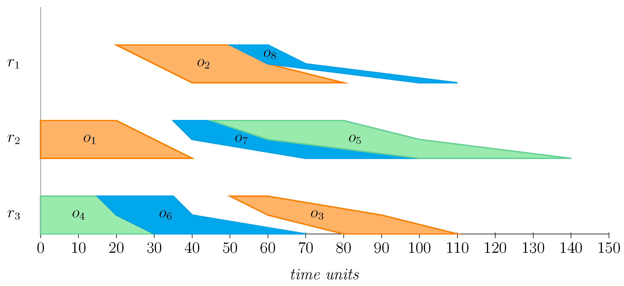
Let us illustrate the three different ways in which $\widehat{CIT}$ can be computed with a toy example. Suppose that we have the schedule $\varphi$ depicted in Figure 2, comprising eight operations scheduled in three resources. To represent the different values of the operations in the schedule, we will use grids as the following:

$$\left[\begin{array}{ccc}{o}_2& o_8& \\ o_1& o_7& o_5\\ o_4& o_6& o_3\end{array}\right]$$

where each row corresponds to the operations scheduled in a resource. This way, the processing times of operations are as follows:

$$\left[\begin{array}{ccc}(30,30,40)& (10,10,10)& \\ (20,30,40)& (10,20,30)& (35,40,40)\\ (15,20,30)& (20,20,40)& (10,30,30)\end{array}\right]$$

Their starting times are given by the following:

$$\left[\begin{array}{ccc}(20,30,40)& (50,60,100)& \\ (0,0,0)& (35,40,70)& (45,60,100)\\ (0,0,0)& (15,20,30)& (50,60,80)\end{array}\right]$$

And their completion times are given by:

$$\left[\begin{array}{ccc}(50,60,80)& (60,70,110)& \\ (20,30,40)& (45,60,100)& (80,100,140)\\ (15,20,30)& (35,40,70)& (60,90,110)\end{array}\right]$$

If we compute operations’ idle times, ${\widehat{I}}_{\varphi }^N$, using the naive approach from (16), we obtain the following values:

$$\left[\begin{array}{ccc}(0,0,0)& (0,0,50)& \\ (0,0,0)& (0,10,50)& (0,0,55)\\ (0,0,0)& (0,0,15)& (0,20,45)\end{array}\right]$$

This results in resource core idle times ${\widehat{CIT}}_{\varphi }^N\left(r_1\right)=(0,0,50)$, ${\widehat{CIT}}_{\varphi }^N\left(r_2\right)=(0,10,105)$, and ${\widehat{CIT}}_{\varphi }^N\left(r_3\right)=(0,20,60)$ and, thus, a total core idle time,

$${\widehat{TCIT}}_{\varphi }^N=(0,30,215).$$

If operation idle times are instead computed with the knowledge-based approach, as proposed in (18), we obtain the following values of ${\widehat{I}}_{\varphi }^K$ for all operations:

$$\left[\begin{array}{ccc}(0,0,0)& (0,0,50)& \\ (0,0,0)& (0,10,50)& (0,0,0)\\ (0,0,0)& (0,0,0)& (0,20,45)\end{array}\right]$$

These yield resource core idle times ${\widehat{CIT}}_{\varphi }^K\left(r_1\right)=(0,0,50)$, ${\widehat{CIT}}_{\varphi }^K\left(r_2\right)=(0,10,50)$, and ${\widehat{CIT}}_{\varphi }^K\left(r_3\right)=(0,20,45)$, so the total core idle time will be

$${\widehat{TCIT}}_{\varphi }^K=(0,30,145).$$

Finally, using the coarse approach to directly compute the core idle time of resources as per (20), we obtain ${\widehat{CIT}}_{\varphi }^C\left(r_1\right)=(0,0,50)$, ${\widehat{CIT}}_{\varphi }^C\left(r_2\right)=(0,10,75)$, and ${\widehat{CIT}}_{\varphi }^C\left(r_3\right)=(0,20,65)$. Then, the total core idle time according to this method is

$${\widehat{TCIT}}_{\varphi }^C=(0,30,190).$$

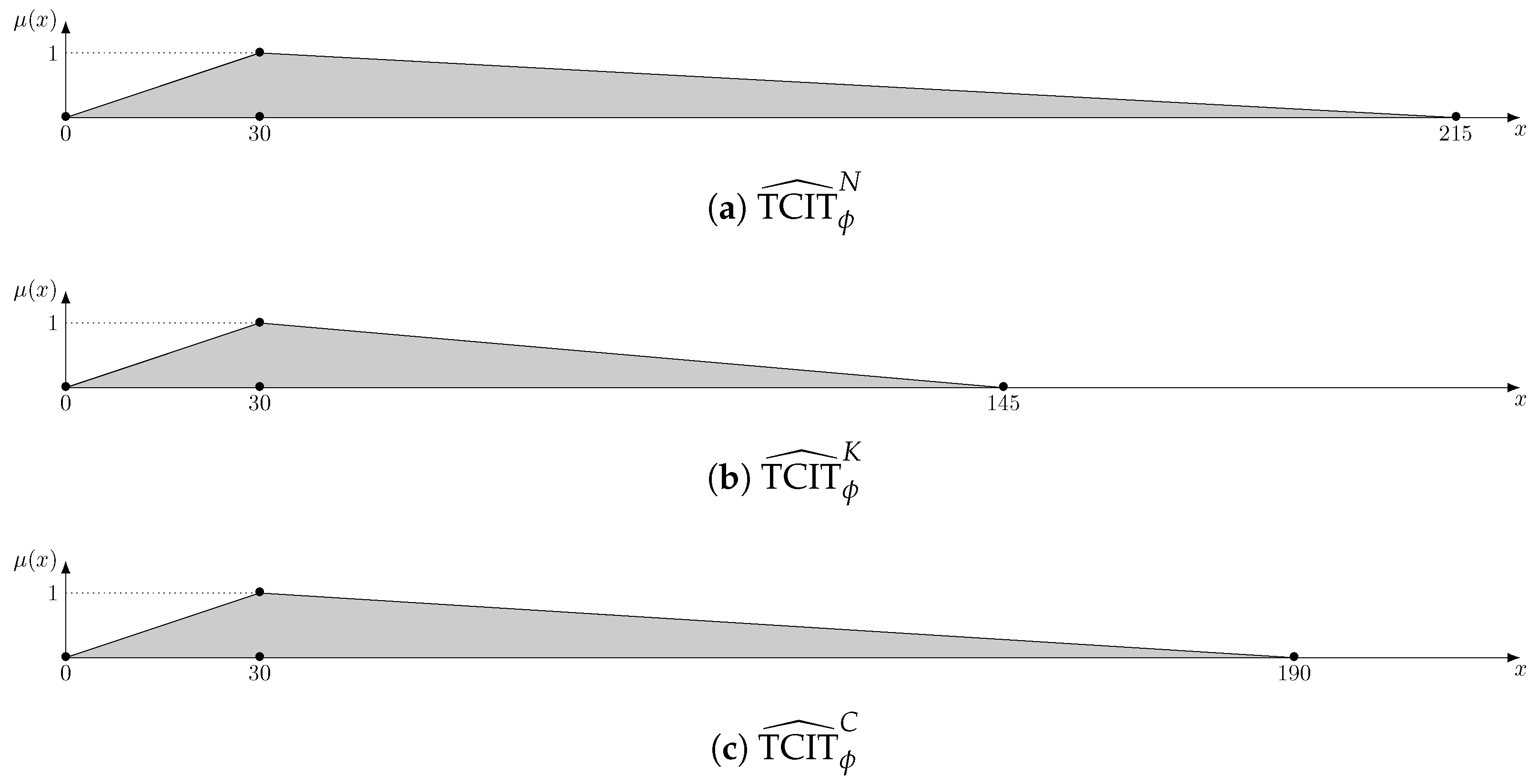
We can appreciate how, unlike the deterministic case, in the fuzzy framework, each approach yields a different value for $\widehat{TCIT}$. The three different TFNs can be seen in Figure 3. It is clear that the support (and, hence, the spread) of the resulting TFN is different in each case. Given their definitions, it is guaranteed that the spread of ${\widehat{TCIT}}_{\varphi }^K$ will always be less than or equal to the spread of ${\widehat{TCIT}}_{\varphi }^N$, i.e., computing the total core idle time with the knowledge-based approach accumulates less uncertainty, as illustrated by the example. In this particular case, the spread for ${\widehat{TCIT}}_{\varphi }^C$ is also larger than the one for ${\widehat{TCIT}}_{\varphi }^K$. However, it is not guaranteed that this will always be so, as shown in the experimental results in Section 4. The example also illustrates that the modal value of ${\widehat{TCIT}}_{\varphi }$ is always the same, regardless of the approach used to compute it. This is a direct consequence of how arithmetic operations are performed on TFNs. Finally, notice how, by truncating negative values, in all three cases, uncertainty accumulates towards the right-hand side, resulting in skewed TFNs.

4. Results

The objective of the experimental study is to empirically assess the three different approaches introduced in Section 3 in order to compute the total core idle time for fuzzy schedules. We will use 12 benchmark instances from the literature [25]: 07a, 08a, 09a, 10a, 11a, and 12a with 15 jobs, 8 resources, and 293 operations (denoted as $15\times 8\times 293$ in the following) and 13a, 14a, 15a, 16a, 17a, and 18a of size $20\times 10\times 387$. In instances 07a, 08a, 09a, 13a, 14a, and 15a, operations have the same processing time, regardless of the resources where they are executed, while instances 10a, 11a, 12a, 16a, 17a, and 18a have resource-dependent processing times. There are also three increasing flexibility levels, with 07a, 10a, 13a, and 16a being those instances with the lowest flexibility and 09a, 12a, 15a and 18a being those instances with the highest flexibility.

The study follows the methodology proposed in [26]. For each instance, schedules will be generated and compared in terms of their performance regarding $\widehat{TCIT}$ using first the measures introduced in Section 2.3.1 and then those introduced in Section 2.3.2. In both cases, this will be done with two types of experiments: over random solutions and with solutions obtained with a search algorithm. The goal of the random-solution experiments is to evaluate the three alternatives for computing $\widehat{TCIT}$ without the possible bias that may be introduced via any solver, whereas the searched-solution experiments pretend to compare the three models when embedded in a search algorithm, with the objective of evaluating their capability of guiding the search towards good schedules. In both sets of experiments, 100 schedules are obtained per instance; notice that, for the searched-solution comparisons, this means generating 100 schedules for each of the three models (${\widehat{TCIT}}^N,{\widehat{TCIT}}^K$, and ${\widehat{TCIT}}^C$) under consideration.

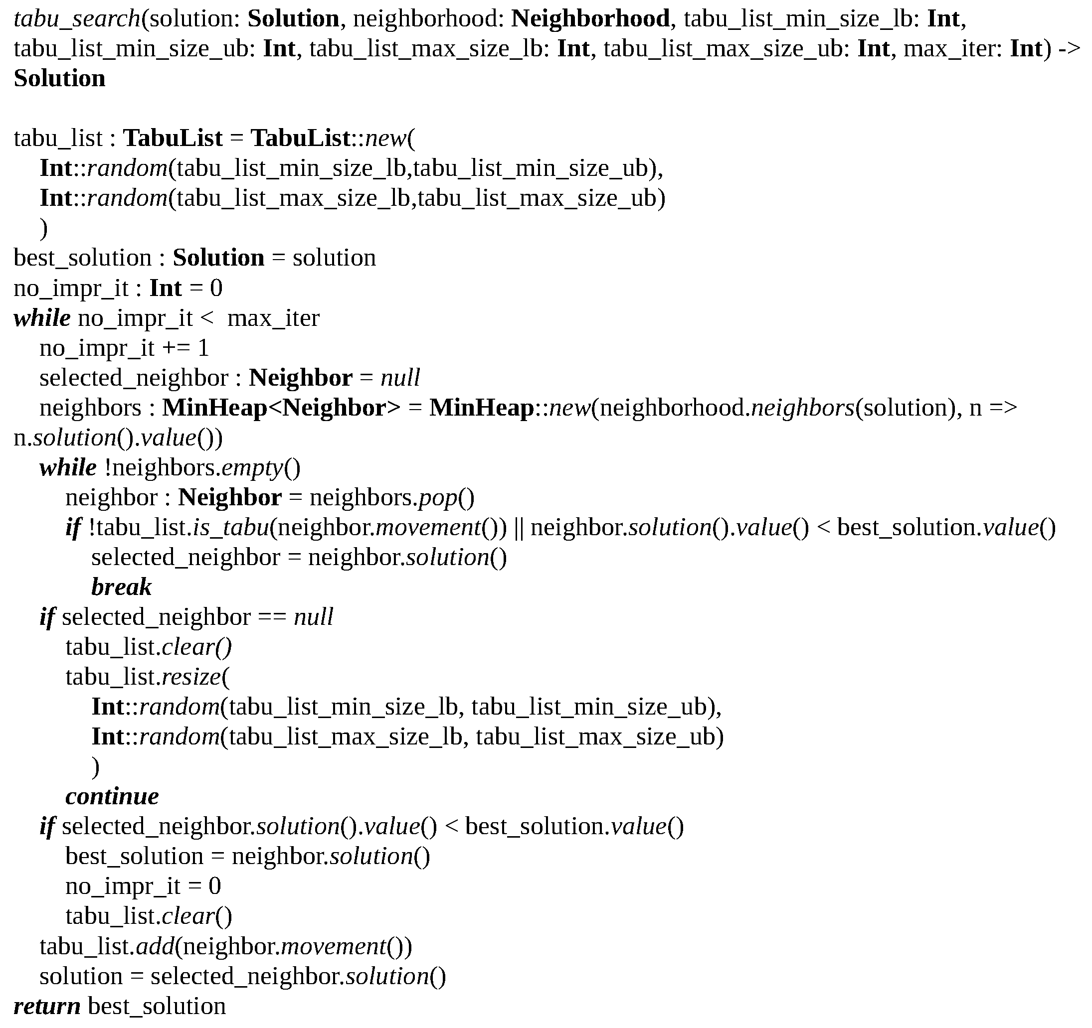
As a solution method for the searched-solution comparisons, we employ the tabu search algorithm proposed in [51] for the classical job shop, extending the neighbourhood function so that every operation is moved to all feasible positions both in its current resource and in others where it can be executed. This is probably the most naive neighbourhood available, as it tries to reschedule every operation in every position, but at the same time, it ensures connectivity and is agnostic to the models, minimising their influence on the results. At every iteration, a tabu search generates all possible neighbours and selects the best one that is not tabu. Then, it stores the inverse of the move performed to obtain the selected neighbour in a memory structure, called the tabu list, so, in the next iterations, that move is forbidden, thus avoiding the undoing of recently made moves. In this way, the tabu search is able to escape local optima. In addition, the tabu list also serves as a diversification mechanism, as different movements are encouraged. A detailed pseudocode can be found in Figure A1. The tabu search parameters are set to the values used in [26] for the same set of instances. This algorithm will be used in all experiments, with the only change being the objective function, which will vary in order to test the different proposals.

4.1. Comparisons Based on Fuzzy TCIT Values

As mentioned in Section 2.3.1, fuzzy TCIT values can be compared in terms of their expected value, their spread, S, and their modal value position, $MVP$.

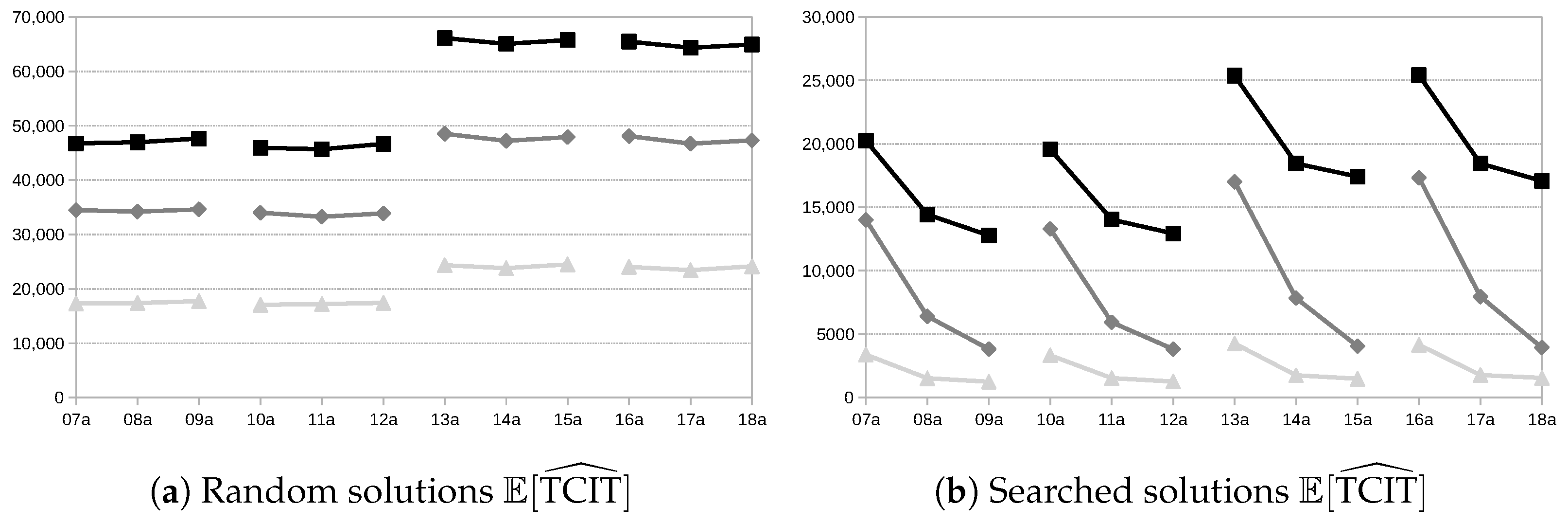
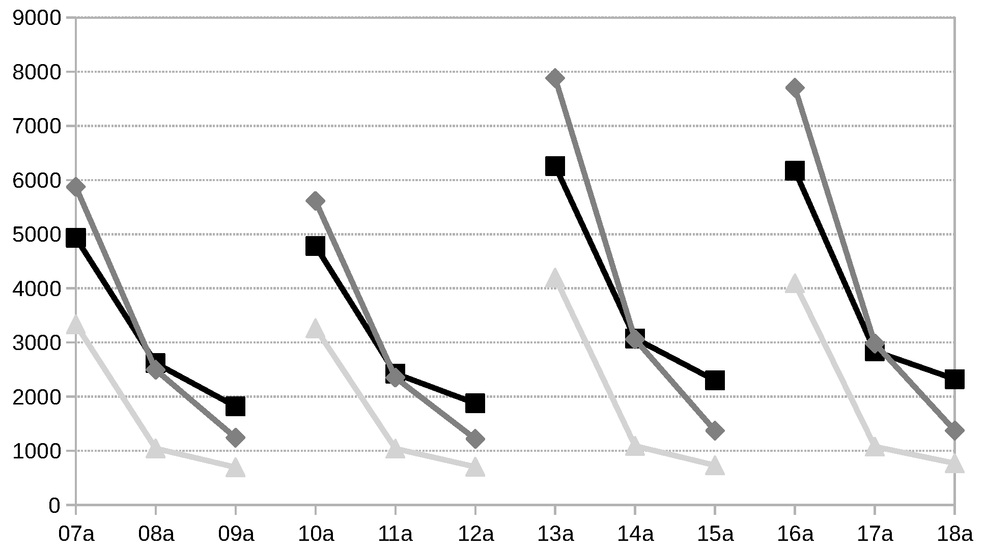
Figure 4 shows the average $\mathbb{E}\left[\widehat{TCIT}\right]$ values obtained for each instance in the two types of experiments. Figure 4a corresponds to the average values obtained when evaluating the random schedules with the three models for computing $\widehat{TCIT}$. Figure 4b depicts average values obtained when evaluating the schedules obtained with the tabu search using each of the three models. In both experiments, there is clearly a difference between the three methods for computing the fuzzy TCIT: ${\widehat{TCIT}}^C$ yields better average expected values than ${\widehat{TCIT}}^K$, and this, in turn, yields better values than ${\widehat{TCIT}}^N$.

Furthermore, for the random solutions experiment, the variation in the expected value seems to depend only on the problem size and not on the flexibility level, as illustrated by the flat lines. This makes sense since, the larger the number of operations, the larger the number of possible gaps, and, as they are not optimised in any way, the longer the total idle time. However, for the searched-solution experiment, differences exist depending not only on the instance size but also on the flexibility level. This may be because greater flexibility provides the search algorithm with more opportunities to move operations between resources and fill inactivity gaps, thus reducing the total core idle time. It is remarkable that, here, ${\widehat{TCIT}}^K$ seems to yield better improvements when greater flexibility is introduced, coming closer to ${\widehat{TCIT}}^C$. On the other hand, the improvement of the naive approach ${\widehat{TCIT}}^N$ does not seem to be as pronounced when flexibility increases. Also, ${\widehat{TCIT}}^K$ expected values are significantly higher than ${\widehat{TCIT}}^C$. This is expected because, although ${\widehat{TCIT}}^K$ has been defined to reduce artificial uncertainty due to dependencies between operations, there are still relations that we cannot easily account for. Thus, the sum of idle times between operations, that is the sum of multiple subtractions, is going to have predictably more artificial uncertainty than the coarser approach, which only makes one subtraction, as the results demonstrate.

When the spread is considered, the obtained graphs are very similar. The reason is that, in these benchmark instances, operations have similar-magnitude processing times with different values for each of the three components of the TFNs. As computing starting times according to Equation (11) are accumulative, the greater the number of already-scheduled operations, the larger the expected value of the TFN and the difference between the first and third components. Then, as the subtraction according to Equation (3) is computed by crossing the value of the lower and upper values of the two TFNs involved, it is predictable that larger expected values also mean larger spread values.

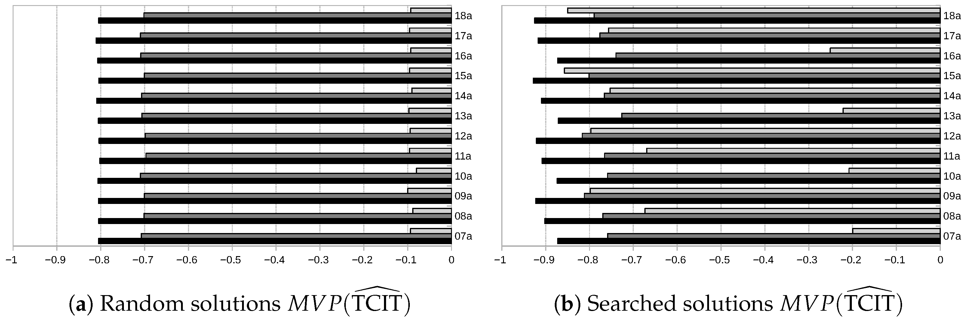
Finally, Figure 5 shows the $MVP$ values obtained in the experiments. Notice that, both in the random solutions and the searched solutions experiments, $MVP$ is negative, meaning that the modal point is situated to the left of the support’s midpoint; i.e., the TFNs are skewed to the right. The main reason for this behaviour is that, in all functions, we are removing negative values because negative times are not possible, but this trimming will only take place on the left side of TFNs. Also, notice that, in the searched-solution experiments, the absolute value of $MVP$ is closer to −1 compared to the random solutions. This is because better solutions mean smaller gaps between operations in the same resource, and then, the probability for the predecessor in the resource being the operation defining the starting time is higher, introducing a dependency between these operations that increases the chances of having negative numbers for idle times. However, the conclusion should not be that being closer to $-1$ is better. The reason is that the processing times of operations are almost symmetrical, but $\widehat{TCIT}$ does not maintain this symmetry, which means that we are accumulating artificial uncertainty on one of the sides. Notice that this effect is aggravated when there is higher flexibility, and that it is much more pronounced for ${\widehat{TCIT}}^C$. This phenomenon can be illustrated as follows. Suppose that, during the tabu search, there is a resource where an operation can be scheduled without altering the starting time of the first operation already scheduled in the resource or the completion time of the last operation in the resource. Then, the minuend in (20) (i.e., the time span between the start of the first operation and the end of the last one) is not altered, while the subtrahend, the sum of processing times of operations assigned to the resource, grows. In consequence, the first component of the difference will be smaller, more likely negative, and, therefore, more likely to be truncated to 0, resulting in a TFN more skewed to the right. When the flexibility level is low, so is the possibility of moving operations to a different resource, while higher flexibility increases the options to move operations between resources, leading to the described behaviour.

4.2. Comparisons Based on Crisp Scenarios

We now evaluate the three models for computing $\widehat{TCIT}$ using the measures described in Section 2.3.2. To this end, we will use a unique set of 1000 crisp possible scenarios, $\mathbf{S}$, derived from the fuzzy instances. These scenarios are generated by setting the processing time of every operation in each allowed resource to a random value derived from a uniform distribution in support of the TFNs.

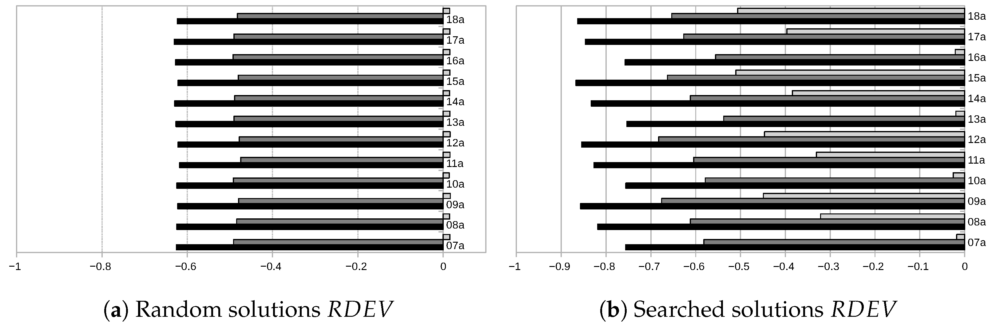
Figure 6 shows, for each instance, the average $RDEV$ across all scenarios in $\mathbf{S}$, both for the random and searched solutions experiments. Clearly, both the results obtained with ${\widehat{TCIT}}^K$ and ${\widehat{TCIT}}^C$ on the crisp scenarios are closer to the predicted expected value than those obtained with ${\widehat{TCIT}}^N$. Those obtained via the coarser approach are the closest to the expected value, evidencing the lower amount of artificial uncertainty that it introduces. One remarkable detail, when comparing random- and searched-solution cases for ${\widehat{TCIT}}^C$, is that, in the random-solution experiment, the relative distance values are positive; i.e., the TCIT values obtained with the executed schedules are, on average, larger than expected. In other words, the predicted estimate provided via ${\widehat{TCIT}}^C$ is slightly optimistic. However, when integrated into the tabu search, the relative deviation becomes negative. As was the case with $MVP$, this can be explained because truncating negative values (which are more likely after an improving local search move) cause the $\widehat{TCIT}$ to be skewed to the right, with a subsequent deviation in the expected values.

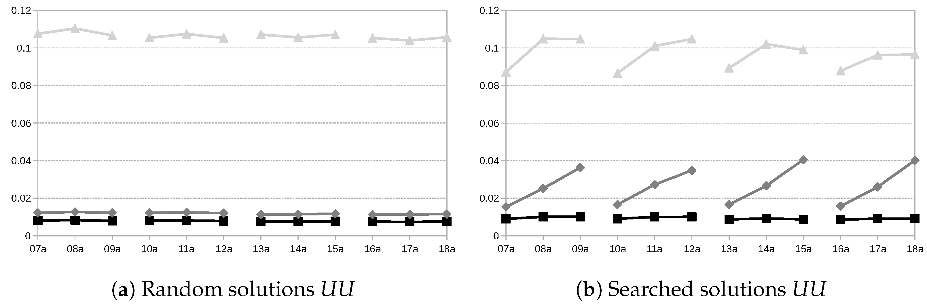
Finally, Figure 7 depicts the results obtained when considering the used uncertainty measure, $UU$. For random solutions, there is no difference in $UU$ with different flexibility levels. However, in the case of searched solutions, there exist interesting differences between the three approaches. In the case of ${\widehat{TCIT}}^K$, increasing flexibility also causes the used uncertainty to increase. However, for ${\widehat{TCIT}}^N$, increasing flexibility does not make any difference in either the random or searched solutions. The case of ${\widehat{TCIT}}^C$ is even more curious, as the initial increase in flexibility allows for higher $UU$, but adding more flexibility can even cause the $UU$ values to decrease. Also, notice that the $UU$ values are quite small. This is because a wider use of the support $\widehat{TCIT}$ would require most crisp realisations for the processing times to be extreme values in the support of each TFN representing processing times, which would contradict the possibility distribution given by each TFN.

In addition to the above assessment, we can also evaluate the crisp TCIT that is obtained with the schedules obtained using the tabu search with each model for computing $\widehat{TCIT}$. The objective is to assess the TCIT that can be obtained according to simulations, rather than using a central tendency measure such as the expected value, which, as we have seen, can be deviated due to the artificial uncertainty that is introduced. Figure 8 shows the average executed TCIT across the 1000 crisp scenarios and the 100 different schedules.

These results show a completely different behaviour with respect to the one observed when comparing based on the fuzzy values. It seems that, according to simulations, in those instances with less flexibility, ${\widehat{TCIT}}^N$ seems to work better than ${\widehat{TCIT}}^K$; however, as flexibility increases, making the problems harder, ${\widehat{TCIT}}^K$ takes the lead. There is no clear explanation for this behaviour other than that instances with less flexibility allow to make very few moves between resources, so most moves in the tabu search are limited to reordering of operations in one resource, and then having less artificial uncertainty in the idle times does not suppose a big advantage, as there would be few chances to find an operation that fills the gap. Meanwhile, ${\widehat{TCIT}}^N$ involves higher artificial uncertainty that skews TFNs more to the right, which means a higher deviation towards the worst case, which, for this set of instances, seems to be a beneficial trait in the guiding function for lower-flexibility cases. In any case, ${\widehat{TCIT}}^C$ remains the dominating alternative and the better approach when the problem at hand does not require computing idle times at the operation level.

5. Conclusions and Future Work

In this work, we have considered the fuzzy flexible job shop scheduling problem, with a focus on computing idle times. We have illustrated the difficulties inherent to computing idle times in the fuzzy framework, caused by operating with interactive uncertain variables. Starting from a naive definition of idle time before an operation from the literature, we have proposed an alternative way to compute such idle time that takes into account existing knowledge about schedules. These two means of computing idle times before operations yield two different ways of computing the core idle time of a resource and, by extension, the total core idle time of a schedule. Additionally, we have proposed a way of directly computing the core idle time in a resource (and, hence, the total core idle time of a schedule) for those cases where not that much granularity is necessary. We have argued that, although, in the deterministic setting, all three of these approaches are equivalent and yield the same value for the total core idle time in a schedule, that is not the case in the fuzzy setting. We finally conducted an experimental study to empirically evaluate the three ways of computing idle times in fuzzy schedules. We have seen how both the new proposals from this work seem superior to the naive means of calculating idle times that exist in the literature. On the other hand, neither of the two new proposals can be thought of as being superior to the other one. Moreover, the choice of which to use is heavily dependent on the particular application context. The knowledge-based approach from Section 3.2 allows fine-grained calculations at the operation level, whereas the coarser approach from Section 3.3 is adequate if only calculations at the resource level are needed.

We hope that our proposals provide a solid basis for future research tackling fuzzy flexible job shop problems where idle times play an important role. Additionally, it would be trivial to extend our new approach to computing waiting times for jobs or to adapt them to computing both idle and waiting times in other fuzzy scheduling problems. In particular, being able to compute idle times between operations in fuzzy schedules is crucial to tackling all of those problems that comprise time-of-use tariffs, i.e., problems in which the offer of energy or its cost varies over time.