Nonparametric Probability Density Function Estimation Using the Padé Approximation

Abstract

Estimating the Probability Density Function (PDF) of observed data is crucial as a problem in its own right, and also for diverse engineering applications. This paper utilizes two powerful mathematical tools, the concept of moments and the relatively little-known Padé approximation to achieve this. On the one hand, moments encapsulate crucial information that is central to both the “time-” and “frequency-”domain representations of the data. On the other hand, the Padé approximation provides an effective means of obtaining a convergent series from the data. In this paper, we invoke these established tools to estimate the PDF. As far as we know, the theoretical results that we have proven, and the experimental results that confirm them, are novel and rather pioneering. The method we propose is nonparametric. It leverages the concept of using the moments of the sample data—drawn from the unknown PDF that we aim to estimate—to reconstruct the original PDF. This is achieved through the application of the Padé approximation. Apart from the theoretical analysis, we have also experimentally evaluated the validity and efficiency of our scheme. The Padé approximation is asymmetric. The most unique facet of our work is that we have utilized this asymmetry to our advantage by working with two mirrored versions of the data to obtain two different versions of the PDF. We have then effectively “superimposed” them to yield the final composite PDF. We are not aware of any other research that utilizes such a composite strategy, in any signal processing domain. To evaluate the performance of the proposed method, we have employed synthetic samples obtained from various well-known distributions, including mixture densities. The accuracy of the proposed method has also been compared with that gleaned by several State-Of-The-Art (SOTA) approaches. The results that we have obtained underscore the robustness and effectiveness of our method, particularly in scenarios where the sample sizes are considerably reduced. Thus, this research confirms how the SOTA of estimating nonparametric PDFs can be enhanced by the Padé approximation, offering notable advantages over existing methods in terms of accuracy when faced with limited data.

1. Introduction

Most natural events are stochastic [1] because they involve uncertain interactions of random internal “environments”. To study these events, researchers have applied probability theory, which is a tool encompassing a branch of mathematics that aids in the analysis of the behavior of stochastic events. Probability theory, in particular, and stochastic processes, in general, are among the most fundamental fields of mathematics. They have applications in signal processing, pattern recognition, classification, forecasting, medical diagnosis, and many other applications. In practice, probability distributions find application in diverse fields such as electron emission, radar detection, weather prediction, remote sensing, economics, noise modelling, etc. [2,3,4,5]. Once the probabilistic model is well-defined, subsequent analysis often involves the theory of “estimation” (synonymously, learning, or training, depending on the application domain). Such estimation is always valuable, but it is nonetheless challenging [6], especially when the available data are limited [7,8].

In this context, the PDF of a random variable is central to various aspects of the analysis and characterization of the data and the model. Many studies have emphasized the need for estimating the PDF [9], which is challenging due to the absence of efficient construction methods.

Suppose that $X_N$ is a set of observed data with N samples randomly distributed with an unknown PDF. The given $X_N$ is characterized by its PDF ($f\left(x\right)$) of the underlying random variable, which satisfies the fundamental properties of a PDF:

$$\begin{array}{cc}\hfill {\int }_{-\infty }^{+\infty }f\left(x\right)dx& \hfill =1,\hfill \\ \hfill f\left(x\right)& \hfill \ge 0.\hfill \end{array}$$

(1)

Once the PDF has been estimated based on a well-defined criterion, one also needs an assessment method to compare $f\left(x\right)$ with the set of observed data to identify the accuracy of our estimation. This PDF can be used to study the statistical properties of the dataset, estimate future outcomes, generate more samples, and so on. Numerous methods have been proposed for estimating the PDF, and these can be classified into two approaches, namely, using parametric or nonparametric models

Unlike parametric models, which make assumptions about the parametric form of the PDF, nonparametric density estimation does not assume the form of the distribution from which the samples are drawn [10]. In parametric models, one develops a model to fit a probability distribution for the observed data, followed by the determination of the parameters of this distribution. The procedure is summarized into four steps:

1.

Select some known candidate probability distribution models based on the physical characteristics of the process and known characteristics of the distribution of the available samples.

2.

Determine the parameters of the candidate models.

3.

Assess the goodness-of-fit of the fitted generative model using established statistical tests and graphical analysis.

4.

Choose the model that yields the best results [2,11,12].

However, these methods cannot cover all data because some datasets do not follow specific distributional shapes. As a result, these methods may fail to accurately approximate the true but unknown PDF [3]. Nevertheless, they contribute to solving many applications.

In nonparametric density estimation, we resort to techniques to find a model to fit the idealistic probability distribution of the observed data [13]. For example, a histogram approximation is one of the earliest density estimation methods, introduced by Karl Pearson [14]. Here, the entire range of values is divided into a series of intervals, referred to as “bins”, followed by adding up the number of samples falling into each bin. Although the so-called bin width is an arbitrary value, extensive research has been done to find a robust way to indicate the effective bin width [15,16]. Moreover, some bins will be empty, while others may have few occurrences. Thus, the PDF will ultimately vary between adjacent bins because of fluctuations in the number of occurrences. By increasing the bin size, each bin tends to contain more samples [17]; however, many important details will be filtered out. This weakness causes the inferred PDF to be discontinuous, and so it cannot be viewed as an accurate method, especially if the derivatives of the histogram are required.

These drawbacks led to the development of more advanced methods, such as Kernel Density Estimation (KDE), Adaptive KDE, Gaussian Mixture Model (GMM), Quantized Histogram-Based Smoothing (QHBS), and the one-point Padé approximation model [18].

KDE [19] is a common density estimator resulting in smooth and continuous densities. It estimates the PDF by deploying a kernel function at each data point and then computing the sum of these kernels to construct a nonparametric estimate of the PDF. The kernel is usually a symmetric, differentiable function, such as the Gaussian. The bandwidth hyperparameter, which defines the width of the kernel, is crucial in determining the smoothness of the resulting estimate.

Adaptive KDE [20] is a form of KDE in which the bandwidth is not constant but instead changes according to the local density of the data. This approach allows for a more accurate depiction of the features of the distribution, especially in regions with dense data, while producing a smoother estimate where there are fewer data points.

GMM [21,22] is a parametric density estimation technique that assumes that the data have been produced by a weighted sum of Gaussian distributions. GMM models the mixture density by estimating the parameters of the (assumed) source Gaussian distributions. Each component of the mixture in the form of Gaussian has its own mean and covariance, while the overall density function is the weighted sum of these individual Gaussian densities. GMM offers a number of advantages over other models and can capture more complex and multi-modal distributions. It is, however, a parametric approach whose accuracy depends on the degree to which its underlying assumptions are met.

QHBS [23] is an approach to address the challenges posed by conventional histograms. It approximates the PDF by smoothing a histogram in a manner that reduces the discontinuities and enhances the smoothness of the resulting density estimate. This approach splits the data into sets of bins and then employs a quantization procedure to soften the estimates and thus produce a smoother, continuous, and differentiable representation of the PDF.

Each of these methods has its strengths and challenges. For instance, while KDE and Adaptive KDE offer smooth and continuous density estimates, selecting the appropriate kernel function and bandwidth can be difficult. On the other hand, methods like GMM and QHBS can address multimodal and discontinuous distributions effectively, but GMM requires knowledge of the number of component distributions, while QHBS is sensitive to the number of bins used in the underlying histogram. Despite these challenges, these methods are widely used in practice due to their ability to provide accurate and flexible density estimates in various applications.

Although we have presented only a rather brief review of these schemes, it can serve as a backdrop to our current work. In this paper, we shall argue that, unlike the previous methods, the use of the moments of the data can serve to yield an even more effective method to estimate the PDF, which also quite naturally leads us to the Padé transform, explained below. Note that we will synonymously refer to this phenomenon as the Padé approximation and the Padé Transform. Amindavar and Ritcey first proposed the use of the Padé approximation for estimating PDFs [24]. We include Amindavar’s original method in our quantitative evaluations below, here referred to as the “one-point Padé approximation model”. As originally formulated, this approach suffers from several challenges, which are mentioned in [24]. First, the Padé approximation method is only applicable to strictly positive data. Second, this method exhibits substantial distortion on the left side of the approximated PDF. Third, the original method did not demonstrate accurate PDF modelling when moments must be estimated directly from sample data. As detailed below, our proposed approach overcomes these challenges to arrive at a novel density estimation technique.

1.1. Organization of the Paper

In the next section, we briefly recall the basic concepts of the Padé approximation and moment estimation, both of which are used frequently in this research, and will be necessary for developing our proposed method. The subsequent section will illustrate the one-point Padé approximation method, which is an essential section to facilitate understanding of the concepts of our work. After that, the proposed method is introduced in reasonable depth. To demonstrate the efficiency of our work, we examine our work by invoking several criteria. Thereafter, the comparison between the proposed method and some of the mentioned methods will be presented. As shown in Section 5, the proposed method is a robust, accurate, and automatic way to estimate the PDF. It would be an efficient way to find an unknown PDF for many applications, especially if the sample size is small.

1.2. On the Experimental Results

It is prudent if we say a few sentences about the datasets, distributions, and experimental results that we have presented here. It is, of course, infeasible and impossible to survey and test all the techniques for estimating PDFs, and to further test them for all the possible distributions. Rather, we have compared our new scheme against a competitive representative method in the time domain. With regard to the frequency domain, we have compared our scheme against the Padé approximation, whose advantages are discussed in a subsequent section. Further, all the algorithms have been tested for four distributions with distinct properties and characteristics, namely Gaussian mixtures, the beta, the Gamma, and the exponential distribution.

2. Mathematical Background

In this section, we briefly present the mathematical foundations of the phenomena used here, namely that of Moments and of the Padé Transform in Section 2.1 and Section 2.2, respectively.

2.1. Moments

Moments are a set of statistical parameters used to describe a distribution [25]. They provide information about the statistical characteristics of a distribution, which is used in many applications. Let $f\left(x\right)$ be the PDF of the random variable x. Then, for the continuous function $f\left(x\right)$, the MGF at zero is defined as:

$$\begin{array}{c}\hfill M_n=E\left(x^n\right)={\int }_{-\infty }^{\infty }{x}^{n}f\left(x\right)dx.\end{array}$$

(2)

In practical scenarios, we encounter two main challenges. Firstly, the PDF of the random variable x is often unknown. Secondly, access to samples is typically limited. In many cases, when estimating moments, we resort to the discrete form of finding the MGF. Assuming we have N samples, the $n\mathrm{th}$ moment can be estimated as follows:

$$\begin{array}{c}\hfill M_n=\widehat{E}\left(x^n\right)={\displaystyle \frac{1}{N}}\sum _{i=1}^N{x}_i^n.\end{array}$$

(3)

While the number of moments is infinite, we will focus on utilizing a subset of these moments. Later, we will leverage these moments to describe the PDF, and thereafter, to the Padé Transform.

2.2. The Theoretical Aspects of the Padé Transform

The Padé approximation (or Transform) is a significant mathematical tool developed by Henry Padé around 1890 [26]. It finds numerous applications in engineering [27], but in the interest of brevity these are not detailed here. The concept of the Padé approximation involves representing a function in a rational form of the corresponding Taylor series expansion. There are several compelling reasons to use the Padé approximation. Firstly, it can be applied to accelerate the convergence of series. More interestingly, even in cases where a series does not converge, the Padé approximation can be employed and yields a good approximation that does converge. Secondly, the Padé approximation represents a rational form of a function, simplifying the problem in many instances. In this regard, the Padé approximation is a valuable tool for approximating functions [28], which is precisely the arena in which we are operating. It is fascinating that the existence of this rational function is derived from Cauchy’s representation of analytic functions [24], and there is an equivalence of the Cauchy integral with the Riemann integral.

$$\begin{array}{c}\hfill h\left(u\right)={\displaystyle \frac{1}{2\pi i}}{\int }_C{\displaystyle \frac{h\left(u^{\prime }\right)}{u^{\prime }-u}}d{u}^{\prime }.\end{array}$$

(4)

In this equation, C represents a contour in the complex plane, over which the integration is performed. This equation holds true for all analytic functions. When employing the Riemann integral, this equation transforms into a rational function, as shown below:

$$\begin{array}{c}\hfill h\left(u\right)={\displaystyle \frac{1}{2\pi i}}\sum _n{\displaystyle \frac{h\left(u_n\right)}{u_n-u}}\Delta u_n,\end{array}$$

(5)

where n is an index that runs over a set of discrete points, $u_n$, in the complex plane. Each point, $u_n$, corresponds to a specific value in this set, and the sum ${\sum }_n$ represents the contribution of all these points to the value of the function $h\left(u\right)$. We can thus see that all analytic functions can be transformed into rational functions. Later, we will observe that this conversion is essential for the convergence of $f\left(x\right)$ and for finding the inverse Laplace transformation. But for the present, we assume that we are given a power series representing an analytic function $f\left(u\right)$:

$$f\left(u\right)=\sum _{i=0}^{\infty }{c}_i{u}^n.$$

(6)

Our goal is to find a rational function, $P^{(L/M)}\left(u\right)$, to represent the series in the form of the Padé approximation function:

$$P^{(L/M)}\left(u\right)={\displaystyle \frac{{\sum }_{n=0}^L{a}_n{u}^n}{{\sum }_{n=0}^M{b}_n{u}^n}},$$

(7)

where L and M are the maximum degrees of the denominator and numerator, respectively. Now, to find $a_n$ and $b_n$, we equate the RHSs of Equations (6) and (7) as:

$$\sum _{i=0}^{\infty }{a}_i{u}^n={\displaystyle \frac{{\sum }_{n=0}^L{a}_n{u}^n}{{\sum }_{n=0}^M{b}_n{u}^n}}=\sum _{i=0}^{L+M}{c}_i{u}^n+O\left(u^{L+M+1}\right).$$

(8)

For this equation, we need $L+M$ coefficients [22]. Since we are dealing with practical problems, we assume that we have a finite number of available coefficients, and ignore the others. More specifically, $O\left(u^{L+M+1}\right)$ represents the remaining terms that we have ignored in Equation (8). To obtain coefficients, we equate the two sides as:

$$\left(\sum _{n=0}^M{b}_n{u}^n\right)\left(\sum _{n=0}^{L+M}{c}_i{u}^n\right)=\sum _{n=0}^L{a}_n{u}^n.$$

(9)

By matching the coefficients, this system of linear equations can be solved easily using the so-called Hankel matrix:

$$\left[\begin{array}{cccc}{C}_{(L-M+1)}& C_{(L+M+2)}& \cdots & C_L\\ ⋮& ⋮& ⋮& ⋮\\ C_{(L-M+K)}& C_{(L-M+K+1)}& \cdots & C_{(L+K-1)}\\ ⋮& ⋮& ⋮& ⋮\\ C_L& C_{(L+M)}& \cdots & C_{(L+M-1)}\end{array}\right]\left[\begin{array}{c}{b}_M\\ ⋮\\ b_K\\ ⋮\\ b_1\end{array}\right]=-\left[\begin{array}{c}{C}_{(L+1)}\\ ⋮\\ C_{(L+K+1)}\\ ⋮\\ C_{(L+M)}\end{array}\right]$$

(10)

These equations calculate the coefficients of the denominator of Equation (8). To find the coefficients of the numerator of Equation (8), we apply Equation (10) to Equation (9) to yield:

$$a_j=C_j+\sum _{i=1}^{min(M,j)}{b}_i{c}_{(j-i)}0\le i\le L$$

(11)

Therefore, by finding the coefficients, we can see how a Taylor series can be transformed into a rational function. In the next section, we demonstrate how we can leverage the advantages of the rational function for our work, namely to obtain the PDF of the samples by using the one-point Padé approximation and moments estimation.

2.3. Finding the PDF of Samples Using Moments Estimation Function

The one-point Padé approximation [24] was proposed for estimating the distribution of continuous functions, by using the MGF. However, it has some drawbacks. This method fails to provide accurate estimates for all the training samples. Specifically, it only estimates the PDF for positive random variables and is not applicable to negative ones, limiting its applicability to many PDFs. Additionally, the final estimation exhibits substantial distortion near zero (on the left side of the approximation). In this paper, our goal is to address these problems.

In this section, we explain how we can estimate the PDF with the aid of the biased approximation of the moments and the one-point Padé approximation. Indeed, through method refinement, the estimation noise can be reduced, leading to improved performance. To simplify the problem, we initially focus on positive random variables with a finite number of samples. Later, we explore how we can estimate the PDF for datasets comprising both positive and negative values. For the purpose of notation, let $\left\{S_i\right\}$ with N coefficients be a set of samples for which we aim to determine the PDF. Let:

$$S_i=\{s_1,\dots ,s_N\}$$

(12)

Let $M_n$ denote the $n\mathrm{th}$ moment of $S_i$. Further, let $f\left(x\right)$ be the continuous PDF of the random variable X, and $F\left(u\right)$ be its Laplace transformation, defined as:

$$F\left(u\right)={\int }_{x=0}^{\infty }f\left(x\right)e^{-ux}dx.$$

(13)

We now expand the exponential function by using its Taylor series. By doing this, and simplifying the equation, we get:

$$F\left(u\right)={\int }_0^{\infty }f\left(x\right)\sum _{n=0}^{\infty }{\displaystyle \frac{{(-u)}^n}{n!}}{x}^{n}dx=\sum _{n=0}^{\infty }{\displaystyle \frac{{(-u)}^n}{n!}}{\int }_0^{\infty }f\left(x\right)x^{n}dx=\sum _{n=0}^{\infty }{M}_n{\displaystyle \frac{{(-u)}^n}{n!}}.$$

(14)

As discussed in Section 2.1, where we briefly introduced the concept of moment estimation, we can use this approach to estimate $M_n$. In the next section, we will demonstrate how we can apply the Padé approximation. The primary reason for using the Padé approximation is that it transforms the infinite series of $F\left(u\right)$ into a rational function, which provides a good approximation which also converges more effectively. The rational function is represented as ${\displaystyle \frac{P_L}{Q_D}}$, where L and D denote the degrees of the numerator and denominator, respectively. Additionally, converting to a rational function enables us to apply the inverse Laplace transform to find $f\left(u\right)$.

2.4. Implementation Considerations of the Padé Transform

The first question that we must resolve is that of determining how many poles and zeros (i.e., the values of L and D) are adequate to yield an accurate approximation. For tackling this issue, we follow the arguments proposed by [29]. For uniqueness and convergence, we limit ourselves to Padé approximations where the degree of the numerator is less than the degree of the denominator. Thereafter, we invoke the residue theorem to find the inverse Laplace transformation as:

$$P_D^L\left(u\right)={\displaystyle \frac{{\sum }_{n=0}^L{a}_n{u}^n}{1+{\sum }_{n=1}^D{b}_n{u}^n}}=\sum _{i=1}^D{\displaystyle \frac{{\lambda }_i}{u+p_i}}.$$

(15)

$${\mathcal{L}}^{-1}\left(P_D^L\left(u\right)\right)=f\left(x\right)=\sum _{i=1}^M{\lambda }_i{e}^{-p_{i}x},p_i>0.$$

(16)

In Equation (15), ${\lambda }_i$ represents the residue associated with each term in the decomposition and $p_i$ denotes the poles of the rational function, where each $p_i$ corresponds to a specific root of the denominator. One major issue with this method is the distortion incurred in estimating the PDF, near zero. As previously discussed, the accuracy of the one-point Padé approximation method is compromised in the right tail; hence, the left tail of the approximation is more reliable and accurate. To illustrate this issue, consider the example of a Gaussian PDF:

$$f\left(x\right)={\displaystyle \frac{1}{\sqrt{2\pi {\sigma }^2}}}{e}^{-{\displaystyle \frac{{(x-\mu )}^2}{2{\sigma }^2}}},$$

(17)

where $\sigma$ and $\mu$ are the standard deviation and mean, respectively, as illustrated in Figure 1, where $\sigma =50$ and $\mu =15$. More specifically, the figure was drawn using 300 samples generated from this distribution. Indeed, we have estimated the PDF and compared it to the ideal (true) one. In Figure 1, we compare the ideal PDF with the estimated one.

As seen in Figure 1, the left part of the estimated PDF does not resemble the shape of the original PDF. Therefore, we require a method to estimate the left part of the PDF accurately. In the next section, we will propose a solution to address this issue. Subsequently, we will compare the proposed method with other methods to assess its effectiveness.

3. The Padé Approximation Using  Artificial Samples

Many branches of science have invoked the Padé approximation as a tool to convert a series into a rational function. Similarly, in our study, we have applied it indirectly to samples to approximate an unknown PDF. The previously discussed method estimated $f\left(x\right)$ using the Padé approximation. However, its accuracy decreases significantly as $x\to 0$, causing distortion in that portion of the PDF. Moreover, all the samples in the previous method must be positive. To resolve this, we propose to utilize two datasets. The first is the given dataset. Thereafter, we create a new dataset from the original one, and the two of them will simultaneously be utilized to solve the problem. Suppose a given sample is randomly distributed from an unknown distribution $f\left(x\right)$ (Equation (18)). We then generate N samples from $R_n$ by mirroring $R_n$ across the y-axis, creating the series $L_n$:

$$R_n=\{x_1,x_2,\dots ,x_N\}.$$

(18)

$$L_n=\{-x_1,-x_2,\dots ,-x_N\}.$$

(19)

As illustrated in Equation (19), all elements of the $L_n$ series will be mirrored values of $R_n$. Consequently, the estimated PDF using the $L_n$ dataset, denoted as $l\left(x\right)$, is precisely the reflection of our PDF function, $f\left(x\right)$, across the negative Y-axis. To address the weakness of the one-point Padé approximation, in the following we will estimate the left part of $f\left(x\right)$ using the right part $l\left(x\right)$. Consequently, we estimate the right part of $f\left(x\right)$ with the help of $R_n$, leading to a more accurate estimation of the function. Now, to calculate $l\left(x\right)$ from $L_n$, we follow the same procedure. To implement the one-sided Laplace transform, firstly, we need non-zero integer samples. Therefore, we shift all elements of $L_n$ by the maximum amount of the $L_n$ series + 1, which is $\beta +1$:

$$L_n=\{-x_1+\beta +1,\dots ,-x_N+\beta +1\}.$$

(20)

Proceeding now from Equation (3):

$$E\left({(-x+\beta +1)}^{n+1}\right)={\displaystyle \frac{1}{N}}\sum _{n=0}^N{(-x+\beta +1)}^n\widehat{x}=-x+\beta +1\widehat{M_n}={\displaystyle \frac{1}{N}}\sum _{n=0}^N{\left(\widehat{x}\right)}^n.$$

(21)

$\widehat{M_n}$ is the moment generating function of our new training samples. So we continue:

$$l\left(u\right)=\sum _{n=0}^{\infty }{\widehat{M}}_n\left({\displaystyle \frac{{(-u)}^n}{n!}}\right)⟶{\widehat{P}}_D^L\left(u\right)={\displaystyle \frac{{\sum }_{n=0}^L{a}_n{u}^n}{1+{\sum }_{n=1}^D{b}_n{u}^n}}=\sum _{i=1}^D{\displaystyle \frac{{\widehat{\lambda }}_i}{u+{\widehat{p}}_i}}.$$

(22)

$$L^{-1}\left({\widehat{P}}_D^L\left(u\right)\right)=l\left(\widehat{x}\right)=\sum _{i=1}^M{\widehat{\lambda }}_i{e}^{-{\widehat{p}}_i\widehat{x}},{\widehat{p}}_i>0.$$

(23)

It is easy to see that $l\left(\widehat{x}\right)$ is the mirrored form of our desired PDF. However, due to the use of the Padé approximation, this estimation suffers from the same issue we discussed before: it is only reliable when $\widehat{x}$ is sufficiently large. Now, our objective is to utilize the right side of $l\left(\widehat{x}\right)$ to replace the distorted part of $f\left(x\right)$. To achieve this, we need to roll back the entire shifting process. Considering Equation (19) and then combining Equation (21) and Equation (15), we have:

$$x=-\widehat{x}+\beta +1\Rightarrow \widehat{x}=-x+\beta +1.$$

(24)

The estimated PDF $\widehat{f}\left(x\right)$ is given by:

$$l\left(x\right)=\left\{\begin{array}{cc}\hfill l(-x+\beta +1),\hfill & \hfill \mathrm{if}x\to 0\hfill \\ \hfill r\left(x\right),\hfill & \hfill \mathrm{if}x\to \infty .\hfill \end{array}\right.$$

(25)

$R\left(x\right)$ is the estimation of the series $R_n$. An acceptable point C is required to be considered as the “centroid” for combining these two functions. The final result is equal to:

$$g\left(x\right)=\left\{\begin{array}{cc}\hfill {\displaystyle \frac{l\left(x\right)}{{\int }_C^{\infty }\left(l\left(x\right)+{\int }_C^{\infty }r(-x+m)dx\right)}},\hfill & \hfill \mathrm{if}x>C;\hfill \\ \hfill {\displaystyle \frac{f(-x+m)}{{\int }_C^{\infty }\left(l\left(x\right)+{\int }_C^{\infty }f(-x+m)dx\right)}},\hfill & \hfill \mathrm{if}x<C.\hfill \end{array}\right.$$

(26)

The denominators of sub-equations are necessary to ensure that the integral of $g\left(x\right)$ is equal to unity. Selecting the best value for C is one of the challenges that should be taken into account. In this paper, we select the mean of $X_n$ because it yields good experimental results. For illustrative purposes, we apply the method in some examples. With this approach, one can approximate the function; however, a discontinuity may arise. The function is not smooth at the point C, and there is a jump at the point C. For illustrative purposes, we first apply the method in one example, and then we highlight the issue. Finally, we propose a method by which we can render the function to be continuous at this point. The ideal Gaussian PDF given in Equation (17) was used to generate normally (Gaussian) distributed samples. Thereafter, we randomly selected 200 samples, $S_{200}$, with the help of an inverse transform sampling method [30].

$$S_{200}=\{x_1,\dots ,x_{200}\}.$$

(27)

$$\begin{array}{cc}\hfill R_{200}& =\{x_1,\dots ,x_{200}\},\hfill \\ \hfill L_{200}& \hfill =\{-x_i+max\left(R_{200}\right)\mid 1\le i\le 200\}.\hfill \end{array}$$

(28)

These two sets, namely $R_{200}$ and $L_{200}$, are samples that are generated to calculate the right and left parts of the PDF, respectively. As shown in Figure 1, after applying the approximant method, the left and right parts of the PDF are calculated separately. For example, $\left\{L_{200}\right\}$ is the dataset utilized to draw the left part of the PDF.

$$N(50,10)={\displaystyle \frac{1}{\sqrt{2\pi \times 10}}}{e}^{-{\displaystyle \frac{{(x-50)}^2}{200}}}.$$

(29)

In the same vein, $f_L\left(x\right)$ and $f_R\left(x\right)$ are functions that draw the left and right sides of the learned PDF, respectively. After performing this operation, we obtain:

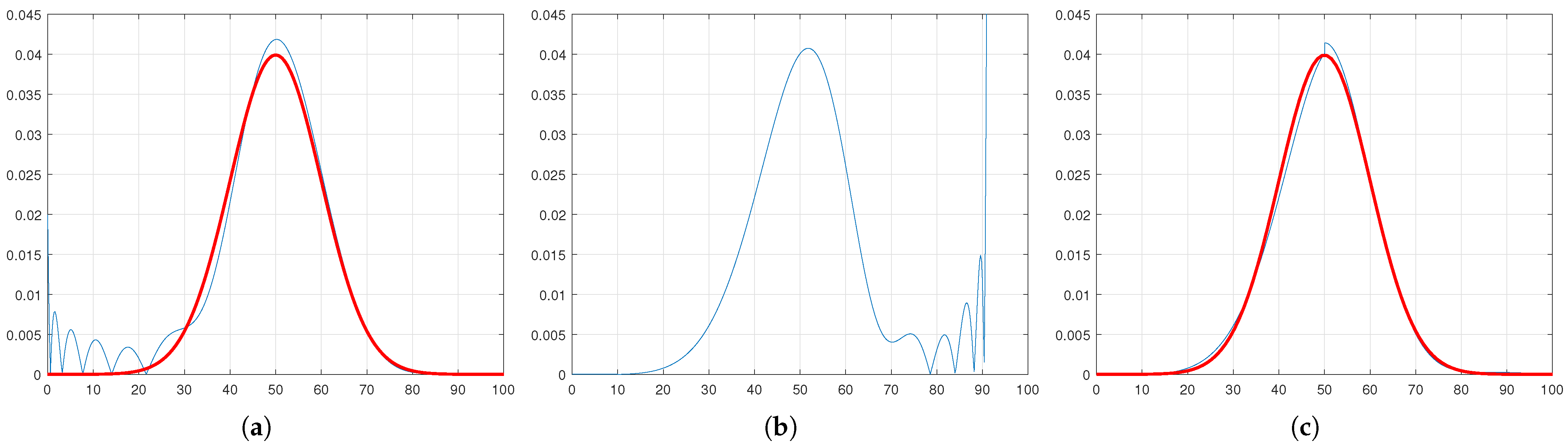
$$\begin{array}{cc}\hfill f_L\left(x\right)& =7200e^{-0.23x}-(255+71i)e^{-0.19-0.13ix}\hfill \\ & +(255-71i)e^{-0.19+0.13ix}+(11+9.2i)e^{-0.15-0.19ix}\hfill \\ & +(11-9.2i)e^{-0.15+0.19ix}+\dots \hfill \end{array}$$

(30)

$$\begin{array}{cc}{f}_R\left(x\right)\hfill & =(88+31i)e^{-0.21-0.11ix}+(88-31i)e^{-0.21+0.11ix}\hfill \\ & -(255+40i)e^{-0.22-0.056ix}-(255-40i)e^{-0.22+0.056ix}+\dots \hfill \end{array}$$

(31)

In Figure 2, we display the left and right parts of the PDF. The blue series represents the ideal PDF, while the red series represents the estimated PDF. Subsequently, these PDFs are combined to create a less noisy PDF; see Figure 2c, which is highly similar to the ideal PDF. However, as we discussed earlier, there is a discontinuity at the midpoint (50). To address this, in the next section (Section 4) we introduce a sigmoid-based smoothing function to eliminate this discontinuity.

4. Using a Sigmoid-Based Transition

When dealing with piecewise functions, abrupt transitions between segments can introduce discontinuities or undesirable behaviour. To achieve a smooth transition between two functions, we can use a sigmoid-based blending approach [31]. This method is particularly useful in scenarios where continuity and differentiability are important, such as in working with PDFs or control systems. The sigmoid function is defined as:

$$\sigma (t,c,k)={\displaystyle \frac{1}{1+e^{-k(t-c)}}}.$$

(32)

The sigmoid function is defined as a smooth, continuous curve that transitions from 0 to 1. Here, t is the independent variable, c is the transition point, and k controls the steepness of the transition. The parameter k determines how sharply the curve transitions. For small values of k, the transition is gradual, blending the functions smoothly over a wider range. For larger values of k, the transition becomes sharper, closely approximating a step function at $t=c$.

To smoothly blend two functions, $f_1\left(t\right)$ and $f_2\left(t\right)$, around the transition point, c, we define the blended function by Equation (33) as:

$$f_{\mathrm{blended}}(t,c,k)=f_1\left(t\right)·(1-\sigma (t,c,k))+f_2\left(t\right)·\sigma (t,c,k).$$

(33)

This formulation ensures that as $t\to -\infty$, $\sigma (t,c,k)\to 0$, and the blended function approaches $f_1\left(t\right)$. Similarly, as $t\to \infty$, $\sigma (t,c,k)\to 1$, and the blended function approaches $f_2\left(t\right)$. Around $t=c$, the two functions are smoothly combined based on the sigmoid weighting. The sigmoid-based transition is commonly used in various applications, such as in control systems, where it facilitates gradual shifts between control regimes, and signal processing, where it is employed for blending signals or applying gradual filters. This approach provides a robust mechanism for creating smooth, continuous transitions between functions, enhancing both stability and interpretability in mathematical models. In our work, we used the sigmoid function for PDF reconstruction. This function ensures smooth transitions between the mirrored and original PDFs, effectively eliminating the discontinuity point.

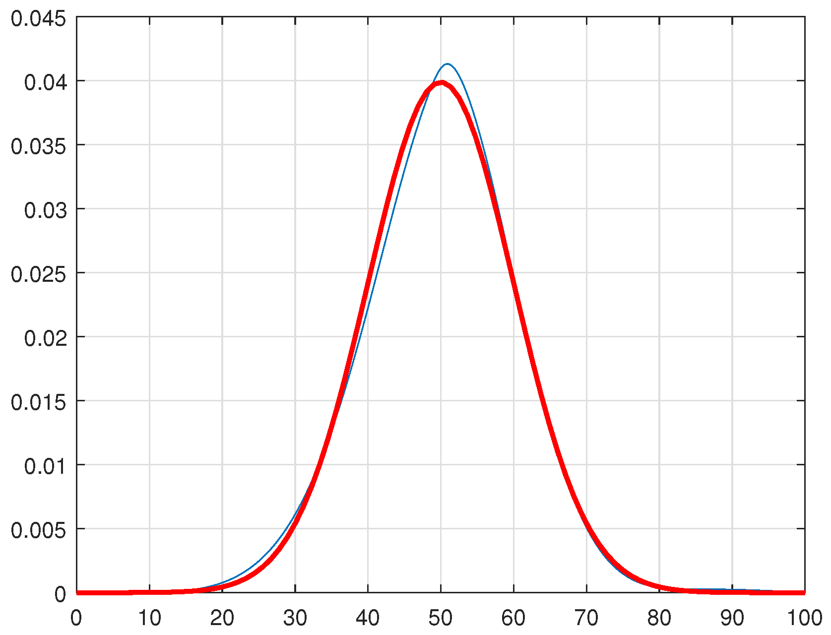
The result of applying the smoothing algorithm to the example from Section 3 is seen in Figure 3.

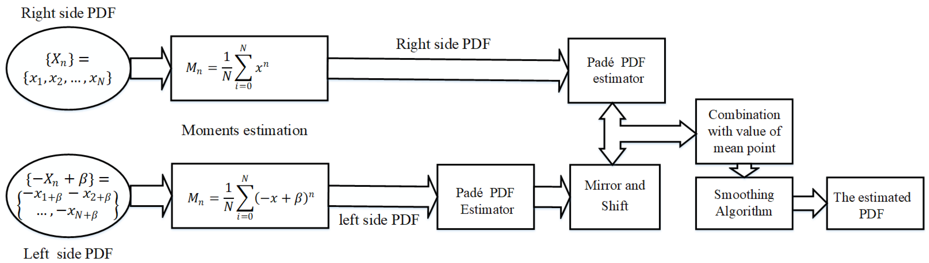
To illustrate the proposed method within the broader context, Figure 4 presents a schematic diagram of the PA procedure. This figure outlines the sequential steps required to achieve an accurate approximation. Specifically, using Equation (33), we depict the final estimation obtained by combining the two estimations.

In addressing the challenge of estimating the probability density function for negative random variables, we utilized a methodology involving horizontally shifting all samples to create a new dataset comprising only positive values. This positive dataset was then utilized to accurately approximate the probability density function. The process was initiated by aggregating all samples with a maximum absolute value, and subsequently, employing the same procedure outlined in Section 3 to estimate the PDF. In the final step, the samples were reverted to their original positions. To illustrate this procedure, consider the example in which $S_{500}$ is a series of 500 samples randomly generated from a Gaussian distribution with a mean of zero and a variance of 20, i.e., ($N(0,20)$).

In the first step, all the samples were transformed into positive samples by shifting by the Min($S_{1000}$), such that they were strictly positive.

$$S_{500}=\{x_1,\dots ,x_{500}\}.$$

(34)

The transformed samples, denoted as $S_n^{\prime }$, were obtained using the following equation:

$$S_n^{\prime }=S_n+\mathrm{Max}\left(S\right)+1.$$

(35)

The proposed method was then applied to this set which results in an estimate of the PDF (see Figure 5).

5. Quantitative and Comparative Assessment

In this section, we report the results obtained by conducting several experiments to assess the performance of the proposed method. The experiments can be summarized as follows. Firstly, the proposed method was applied to datasets generated from well-known probability distributions. The results were then compared with the ideal PDF. Subsequently, the proposed method was compared with other state-of-the-art methods. We aimed to show that our new approach could produce favourable outcomes when working with fewer samples, i.e., in scenarios where data are limited, which is a common occurrence in real-world situations. In addition, we have made the MATLAB code, implementing all the proposed methods, publicly available in the following GitHub repository: https://github.com/hamidddds/Twosided_PadeAproximation (accessed on 23 January 2025).

In our research project, we conducted a series of tests to thoroughly investigate the problem using three datasets of varying sizes. The first dataset consisted of 300 samples, which we categorized as a large dataset, providing a robust representation for comprehensive analysis. The second dataset contained 100 samples, classified as a medium-sized dataset, offering a sufficient number of samples for a balanced evaluation. Lastly, the third dataset comprised only 50 samples, representing a very small dataset specifically designed to simulate challenging scenarios in which access to extensive data is limited. This enabled us to assess how well the performance varied across the sample sizes. In real-world applications, sample sizes of 50 are often insufficient to accurately calculate all data properties in specific ranges. In many cases, scientists address this limitation by making assumptions about the underlying structure of the density and then using parametric methods to estimate the parameters, although the overall accuracy of the results tends to decrease, particularly when incorrect assumptions are made regarding the density. Despite these challenges, we included these small sample sizes to demonstrate that, even in harsh conditions, our method can capture some characteristics of the data and perform reasonably well. However, it is important to note that such small sample sizes are highly sensitive to data sparsity, which can significantly impact performance. Clearly, it is important to mention that the accuracy of all estimations improved with increasing numbers of samples.

In this article, we employ five techniques for comparison with our proposed approach: Kernel Density Estimation (KDE), Adaptive KDE, Gaussian Mixture Model (GMM), Quantized Histogram-Based Smoothing (QHBS), and the one-point approximation model. Since our method is based on the one-point Padé approximation model, we have included it as a reference point for evaluating our approach. The KDE is a nonparametric technique that smooths data points to estimate the underlying PDF without assuming a specific distribution. It employs a kernel function, such as the Gaussian, and a bandwidth parameter to control the level of smoothing. In this study, a Gaussian kernel was used, with the bandwidth calculated using Silverman’s rule of thumb [32]. The Adaptive KDE enhances the standard KDE by dynamically adjusting the bandwidth based on the density of data points. This adaptability enables it to handle varying data densities efficiently, capturing intricate details in densely populated regions while ensuring uniformity in sparser areas. The Adaptive KDE utilized the same Gaussian kernel but varied the bandwidth locally to reflect data density. The GMM is a parametric technique that represents the PDF as a combination of weighted Gaussian components. It estimates the parameters using methods such as expectation–maximization, providing an effective approach for clustering and density estimation. While the GMM performs well when data adhere to Gaussian assumptions, it may face challenges with non-Gaussian distributions. In this study, a three-component Gaussian model was employed, a configuration commonly observed in many applications [33,34,35]. The QHBS combines histogram-based density estimation with smoothing techniques. It divides the data into segments, or bins, estimates the density within each bin, and then applies smoothing to reduce abrupt changes in the data distribution. For this study, the number of bins was set to 20 to balance detail and smoothness [36].

To evaluate the performance of our proposed approach, we utilized six metrics: the Wasserstein Distance, the Bhattacharyya Distance, the Correlation Coefficient, the Kullback–Leibler (KL) Divergence, the L1 Distance, and the L2 Distance. The Wasserstein Distance evaluates the cost of transforming one probability distribution into another by examining variations in their distributions, making it responsive to the distribution’s shape and useful for assessing alignment. A score of zero for the Wasserstein Distance signifies similarity between distributions. The Bhattacharyya Distance measures the overlap between two distributions, helping us understand how well two methods approximate densities by directly reflecting their probabilistic similarity. A smaller Bhattacharyya Distance suggests a better approximation quality, with zero indicating a perfect overlap. The Correlation Coefficient assesses the linear relationship between distributions, providing a clear interpretation of their alignment. A Correlation Coefficient of 1 signifies perfect linear correlation, whereas a value of 0 indicates no linear relationship between them. The KL Divergence measures the difference between two distributions, revealing the drawbacks of approximating one using the other. It is useful for identifying subtle variations in the distribution of probability mass. A lower KL Divergence is preferred, as it signifies greater similarity between distributions, with zero indicating identical distributions. The L1 Distance (also known as Manhattan or Taxicab Distance) calculates the sum of absolute differences between corresponding elements in two vectors or distributions. It is particularly effective in high-dimensional spaces and provides an intuitive measure of dissimilarity. A smaller L1 Distance indicates greater similarity between distributions, with zero representing identical distributions. The L2 Distance (commonly referred to as Euclidean Distance) measures the straight-line distance between two points in a multidimensional space using the Pythagorean theorem. It is widely used for numerical data and provides a geometric interpretation of similarity. Like L1, an L2 Distance of zero indicates identical distributions, while larger values signify greater dissimilarity. These measures collectively provide a comprehensive foundation for assessing the accuracy, reliability, and alignment of density estimation methods across various dimensions and scenarios.

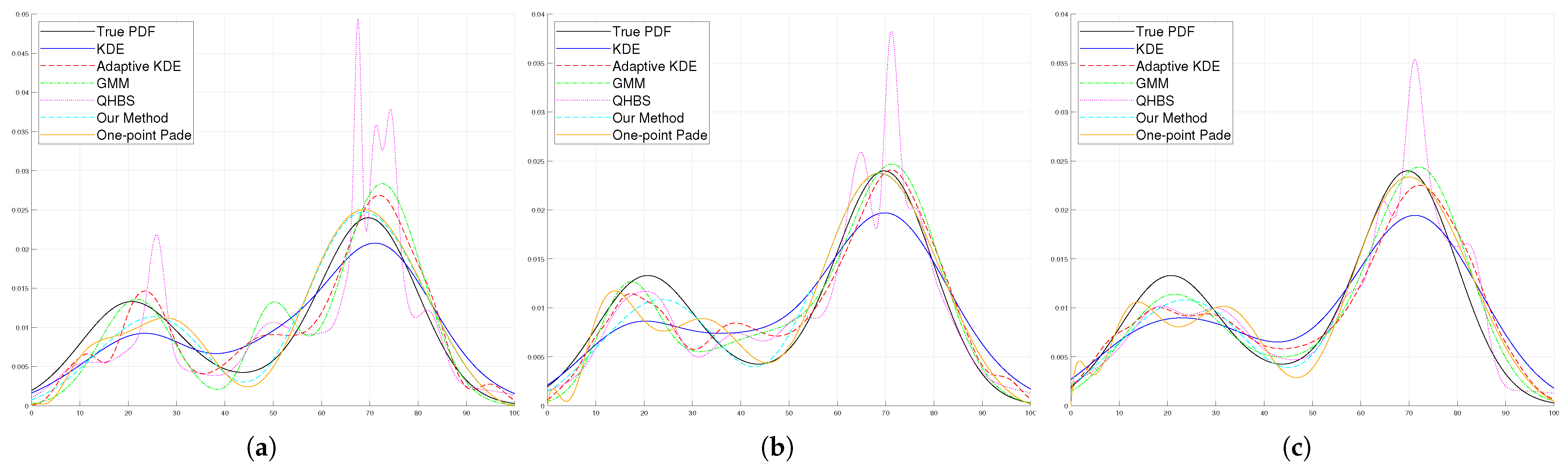
5.1. Example 1: Gaussian Mixture

For the first experiment, we chose a Gaussian mixture distribution model. This is because many real-world problems are based on Gaussian distributions or their combinations so as to simulate real-world problems. The multi-modal distribution was constructed by summing three Gaussian distributions:

$$f\left(x\right)={\displaystyle \frac{1}{0.75}}\left({\displaystyle \frac{1}{2}}N(20,10)+N(40,20)+{\displaystyle \frac{1}{4}}N(70,10)\right)$$

(36)

The value of 0.75 ensured that the properties of a probability distribution were preserved, with its integral being equal to unity. In this equation, $N(\mu ,\sigma )$ represents a Gaussian distribution with mean $\mu$ and standard deviation $\sigma$, as defined in Equation (37). The coefficients before the Gaussian distributions were chosen arbitrarily.

The results of the experiments are displayed in Figure 6.

$$N(\mu ,\sigma )={\displaystyle \frac{1}{\sigma \sqrt{2\pi }}}{e}^{-{\displaystyle \frac{{(x-\mu )}^2}{2{\sigma }^2}}}.$$

(37)

Table 1. Performance metrics for different methods for the Gaussian mixture using 300 samples. Here and elsewhere, bold is used to indicate the best results.

Method	↓ WD	↓ BD	↑ CC	↓ KLD	↓ L1	↓ L2
KDE	32.4425	2.3137	0.9324	0.0045	0.2329	0.0084
Adaptive KDE	28.8019	2.3091	0.9369	0.0029	0.1939	0.0074
GMM	28.2692	2.3050	0.9672	0.0013	0.1312	0.0053
QHBS	30.1941	2.3082	0.9272	0.0026	0.1877	0.0087
One-Point Padé	30.4723	2.3088	0.9496	0.0032	0.1605	0.0065
Proposed Method	31.4479	2.3057	0.9712	0.0016	0.1163	0.0049

,

Table 2. Performance metrics for different methods for the Gaussian mixture using 100 samples.

Method	↓ WD	↓ BD	↑ CC	↓ KLD	↓ L1	↓ L2
KDE	30.5430	2.3143	0.9195	0.0048	0.2430	0.0087
Adaptive KDE	28.4085	2.3094	0.9494	0.0031	0.1782	0.0065
GMM	28.2237	2.3105	0.9501	0.0038	0.1590	0.0068
QHBS	28.9642	2.3102	0.9237	0.0034	0.2033	0.0092
One-Point Padé	28.7078	2.3088	0.9572	0.0036	0.1462	0.0061
Proposed Method	29.5758	2.3049	0.9742	0.0013	0.1185	0.0047

and

Table 3. Performance metrics for different methods for the Gaussian mixture using 50 samples.

Method	↓ WD	↓ BD	↑ CC	↓ KLD	↓ L1	↓ L2
KDE	39.6778	2.3137	0.9191	0.0046	0.2352	0.0083
Adaptive KDE	38.3835	2.3138	0.9243	0.0052	0.2331	0.0086
GMM	39.8234	2.3127	0.9452	0.0049	0.2189	0.0095
QHBS	40.0201	2.3255	0.8182	0.0095	0.3795	0.0170
One-Point Padé	40.4137	2.3102	0.9659	0.0045	0.1729	0.0062
Proposed Method	38.8917	2.3074	0.9672	0.0025	0.1567	0.0059

detail the outcomes for varying sample sizes. We observed that, for small and medium and large sample sizes, our method outperformed the strategies proposed in prior studies. As the sample size increased, the GMM technique surpassed our method in performance. The GMM’s reliance on the underlying distribution has been noted for its effectiveness in estimating Gaussian density functions. However, when handling datasets where the histogram shape diverges significantly from a Gaussian distribution, its accuracy tends to decline. This makes parameter estimation challenging for methods like the GMM. Our method excels in such scenarios, as evidenced by Examples 2, 3, and 4 below. Notably, it produced results without visible distortions at the beginning of the graph, highlighting its robustness under these conditions.

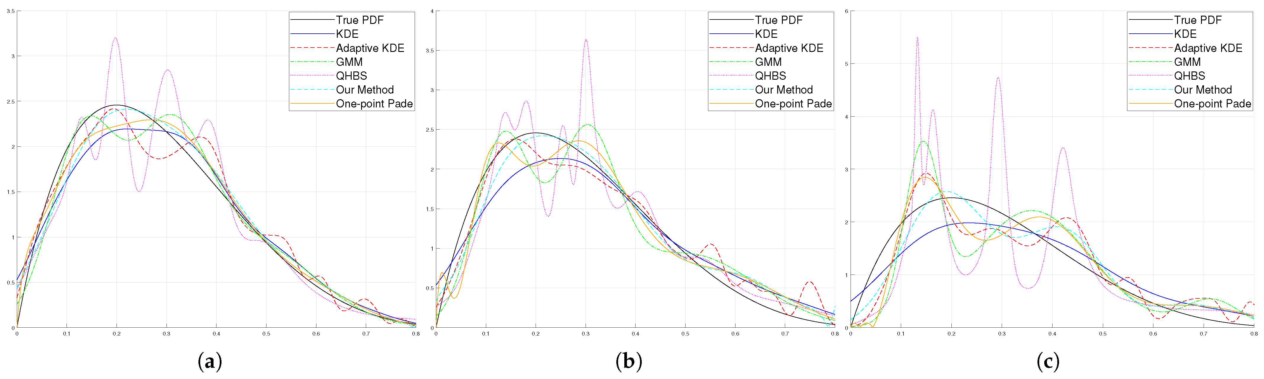
5.2. Example 2: The Beta Distribution

The next distribution model that we consider is the Beta distribution. The Beta distribution is a continuous probability distribution defined on the interval [0, 1], making it suitable for modelling probabilities and proportions. It is governed by two shape parameters, $\alpha$ and $\beta$, which influence the distribution’s shape, allowing it to be symmetric, skewed, or U-shaped. The Beta distribution is extensively utilized in Bayesian statistics as a conjugate prior for binomial and Bernoulli processes, enabling efficient updates of beliefs based on observed data. In our experiment, the parameters were chosen as $\alpha =2$ and $\beta =5$ to evaluate the performance of our method in comparison to other methods. The formula for the PDF of the Beta distribution is shown in Equation (38). The results of the simulations are given in Figure 7.

$$f(x;\alpha ,\beta )={\displaystyle \frac{\Gamma (\alpha +\beta )}{\Gamma \left(\alpha \right)\Gamma \left(\beta \right)}}{x}^{\alpha -1}{(1-x)}^{\beta -1}\mathrm{for}0\le x\le 1$$

(38)

The results (see

Table 4. Performance metrics for different methods for the beta distribution using 300 samples.

Method	↓ WD	↓ BD	↑ CC	↓ KLD	↓ L1	↓ L2
KDE	18.4653	7.1327	0.9844	0.005	0.1070	0.0042
Adaptive KDE	15.7541	7.1331	0.9800	0.017	0.1203	0.0048
GMM	11.6768	7.1313	0.9868	0.009	0.0806	0.0035
QHBS	11.8088	7.1360	0.9356	0.003	0.1780	0.0081
One-Point Padé	13.7342	7.1319	0.9876	0.021	0.0798	0.0034
Proposed Method	11.0687	7.1311	0.9897	0.003	0.0789	0.0032

,

Table 5. Performance metrics for different methods for the Beta distribution using 100 samples.

Method	↓ WD	↓ BD	↑ CC	↓ KLD	↓ L1	↓ L2
KDE	29.5680	7.1375	0.9811	0.012	0.1418	0.0055
Adaptive KDE	33.4228	7.1376	0.9848	0.015	0.1460	0.0055
GMM	28.7827	7.1368	0.9565	0.020	0.1716	0.0063
QHBS	37.6501	7.1395	0.9107	0.025	0.2023	0.0092
One-Point Padé	28.6066	7.1376	0.9644	0.018	0.1503	0.0058
Proposed Method	27.1665	7.1356	0.9856	0.010	0.1105	0.0045

and

Table 6. Performance metrics for different methods for the Beta distribution using 50 samples.

Method	↓ WD	↓ BD	↑ CC	↓ KLD	↓ L1	↓ L2
KDE	41.9417	7.1406	0.9634	0.025	0.2126	0.0074
Adaptive KDE	45.4668	7.1438	0.9130	0.030	0.2402	0.0088
GMM	43.3645	7.1566	0.8302	0.020	0.3128	0.0132
QHBS	51.2981	7.1775	0.6701	0.035	0.5102	0.0225
One-Point Padé	43.3572	7.1519	0.8915	0.018	0.2500	0.0100
Proposed Method	37.9675	7.1405	0.9392	0.015	0.1921	0.0074

) demonstrate that our method outperformed competing approaches and secured first place in the competition. For a sample size of 50, the results indicate that KDE achieved superior performance in terms of the Correlation Coefficient, showing an advantage in this specific criterion. However, across other evaluation metrics our method consistently delivered better performance.

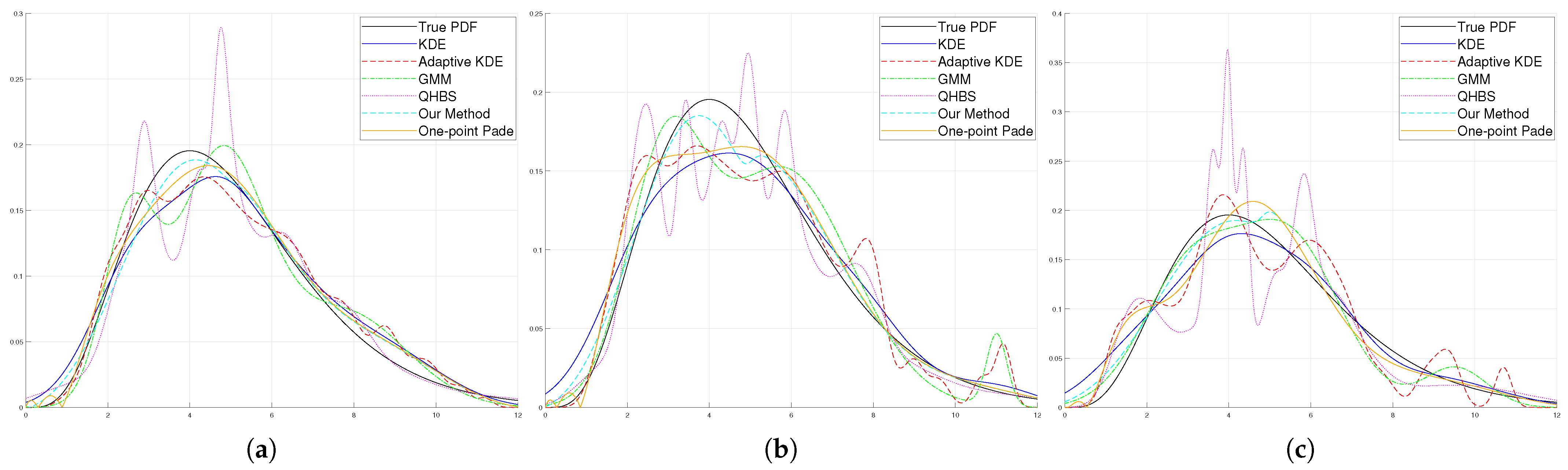
5.3. Example 3: The Gamma Distribution

In our study, we also examined the Gamma distribution, which is recognized for its versatility in effectively representing both symmetrical and skewed datasets. This particular distribution provides valuable perspectives when estimating PDFs. It finds applications in fields such as finance (for predicting waiting durations), engineering (for analyzing failures), and various scientific phenomena that involve the duration until a specific event occurs. Noteworthy is the fact that the Exponential distribution, Erlang distribution, and chi-squared distribution are special cases of the Gamma distribution. The formula for the Gamma distribution is given in Equation (39).

$$f(x;\alpha ,\beta )={\displaystyle \frac{{\beta }^{\alpha }{x}^{\alpha -1}{e}^{-\beta x}}{\Gamma \left(\alpha \right)}},\mathrm{for}x,\alpha ,\beta >0,\Gamma \left(\alpha \right)=(\alpha -1)!$$

(39)

In our experiment, we assumed that $\alpha$ was equal to 5 and $\beta$ was equal to 1. The results, as shown in Figure 8 and

Table 7. Comparison of PDF approximation methods for the Gamma distribution using 300 samples.

Method	↓ WD	↓ BD	↑ CC	↓ KLD	↓ L1	↓ L2
KDE	19.4452	4.4273	0.9888	0.00025	0.1274	0.0053
Adaptive KDE	15.8213	4.4260	0.9840	0.00027	0.1285	0.0051
GMM	14.5563	4.4266	0.9680	0.00033	0.1496	0.0065
QHBS	9.7451	4.4308	0.9265	0.00031	0.1876	0.0101
One-Point Padé	13.4854	4.4250	0.9926	0.00024	0.0899	0.0037
Proposed Method	13.9661	4.4245	0.9950	0.00200	0.0826	0.0032

,

Table 8. Performance metrics for different methods for the Gamma distribution using 100 Samples.

Method	↓ WD	↓ BD	↑ CC	↓ KLD	↓ L1	↓ L2
KDE	18.6965	4.4309	0.9822	0.00265	0.1552	0.0065
Adaptive KDE	15.2305	4.4316	0.9506	0.00285	0.1996	0.0081
GMM	9.8272	4.4266	0.9519	0.00310	0.1474	0.0079
QHBS	8.0250	4.4290	0.9394	0.00360	0.1900	0.0090
One-Point Padé	9.4705	4.4255	0.9772	0.00235	0.1226	0.0057
Proposed Method	7.3515	4.4245	0.9928	0.00205	0.0794	0.0035

and

Table 9. Performance metrics for different methods for the Gamma distribution using 50 samples.

Method	↓ WD	↓ BD	↑ CC	↓ KLD	↓ L1	↓ L2
KDE	12.0644	4.4329	0.9810	0.0250	0.1355	0.0058
Adaptive KDE	12.8983	4.4406	0.9301	0.0300	0.2514	0.0096
GMM	11.0408	4.4308	0.9749	0.0275	0.1451	0.0058
QHBS	15.4045	4.4440	0.8379	0.0350	0.3498	0.0163
One-Point Padé	11.4033	4.4283	0.9657	0.0225	0.1563	0.0067
Proposed Method	10.5327	4.4272	0.9872	0.0200	0.1052	0.0041

, demonstrate the effectiveness of the proposed method, where it outperforms all other methods on all performance metrics and for all sample sizes.

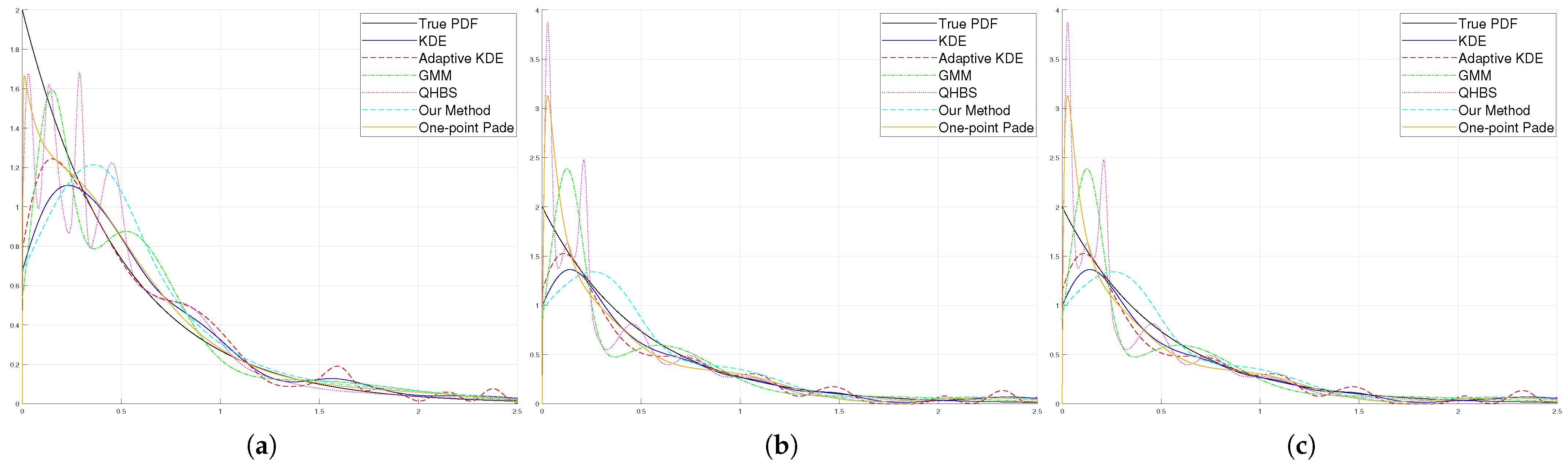
5.4. Example 4: The Exponential Distribution

The above example illustrates the nature of moment-based methods, which are flexible with a limited number of samples. The next distribution model that we consider is the Exponential distribution. The Exponential distribution is commonly used to model the time between events in a Poisson process and is defined by a rate parameter, $\lambda$. The formula for the Probability Density Function (PDF) of the Exponential distribution is shown in Equation (40). In our experiments, $\lambda$ was set to 1. The results of the simulations are given in Figure 9.

$$f(x;\lambda )=\lambda e^{-\lambda x}\mathrm{for}x\ge 0$$

(40)

Upon reviewing the data shown in Figure 7 and

Table 10. Performance metrics for different methods for the Exponential distribution using 300 samples.

Method	↓ WD	↓ BD	↑ CC	↓ KLD	↓ L1	↓ L2
KDE	15.6920	5.3070	0.9526	0.0003	0.2042	0.0197
Adaptive KDE	15.0852	5.3081	0.9716	0.0009	0.1705	0.0158
GMM	9.3181	5.3093	0.9447	0.0003	0.2478	0.0209
QHBS	10.2243	5.3060	0.9769	0.0004	0.1755	0.0135
One-Point Padé	22.2235	5.3160	0.8965	0.0002	0.3207	0.0281
Proposed Method	4.5099	5.3035	0.9819	0.0013	0.0891	0.0120

,

Table 11. Performance metrics for different methods for the Exponential distribution using 100 samples.

Method	↓ WD	↓ BD	↑ CC	↓ KLD	↓ L1	↓ L2
KDE	12.0407	5.3112	0.9802	0.0004	0.2441	0.0128
Adaptive KDE	12.6357	5.3144	0.9461	0.0016	0.1867	0.0206
GMM	10.0232	5.3256	0.9134	0.0008	0.3727	0.0285
QHBS	9.8939	5.3125	0.9213	0.0003	0.2599	0.0295
One-Point Padé	8.9574	5.3130	0.9510	0.0015	0.2252	0.0226
Proposed Method	16.1897	5.3065	0.9829	0.0003	0.1399	0.0119

and

Table 12. Performance metrics for different methods for the Exponential distribution using 50 samples.

Method	↓ WD	↓ BD	↑ CC	↓ KLD	↓ L1	↓ L2
KDE	21.9270	5.3114	0.9694	0.0017	0.1903	0.0157
Adaptive KDE	14.0566	5.3204	0.9579	0.0106	0.2266	0.0195
GMM	20.7139	5.3246	0.9112	0.0009	0.3420	0.0334
QHBS	20.3703	5.3223	0.9123	0.0006	0.3835	0.0339
One-Point Padé	13.4794	5.3203	0.9296	0.0017	0.2398	0.0306
Proposed Method	16.5618	5.3111	0.9897	0.0003	0.1702	0.0102

, it is noticeable that the effectiveness of all techniques has decreased. The main cause for this decline is attributed to the fact that the Exponential distribution presents difficulties in capturing its characteristics near zero, which poses a challenge for the techniques to accurately depict its traits in this region. In some instances, it seems that the One-Point Padé approximation demonstrates better performance. The reason for this could be that the One-Point Padé approximation introduces a distortion near zero, which in this scenario appears advantageous at first glance. The distortion aids in approximating the behaviour near zero to match the characteristics of the Exponential function in that region. Nevertheless, it is crucial to realize that this can give a false impression of enhanced performance, as the distortion does not accurately represent the true nature of the Exponential distribution.

6. Discussion and Conclusions

In this paper, we have considered the problem of estimating the PDF of observed data. Our novel scheme uses two powerful mathematical tools: the concept of moments and the relatively little-known Padé approximation. While moments incorporate crucial information which is central to both the time and frequency domains, the Padé approximation provides an effective means of obtaining convergent series from the data. Both of these phenomena are used in our new method to estimate the PDF in an inter-twined manner.

The method we propose is nonparametric. It invokes the concept of matching the moments of the original function and its learned PDF, and this, in turn is achieved by using the Padé approximation. Apart from the theoretical analysis, we have also experimentally evaluated the validity and efficiency of our scheme.

Although the Padé approximation is asymmetric, we have taken advantage of this asymmetry to our advantage. We have done this by working with two “mirrored” versions of the data so as to obtains different versions of the PDF. We have then effectively “superimposed” (or coalesced) them together to yield the final composite PDF. We are not aware of any other research that utilizes such a composite strategy, in any signal processing domain.

To evaluate the performance of the proposed method, we have employed synthetic samples obtained from various well-known distributions, including mixture densities. The accuracy of the proposed method has also been compared with that obtained by other approaches representative of the families of time- and frequency-domain methods available in the literature.

Our method has shown promising results across the distributions tested. However, we recognize the potential for further exploration. While our chosen examples demonstrate the method’s efficacy, future work could involve testing on a broader range of distributions, including heavy-tailed and multimodal distributions. This extended testing could provide additional insights into the method’s performance under diverse scenarios and potentially uncover new areas for refinement or application.

Moreover, in future research, we intend to explore methods that could enhance the robustness of the proposed approach, particularly in handling outliers. The current method, like other nonparametric density estimation techniques, may be sensitive to extreme values, as sample moments, which can be influenced by outliers. Although this issue can be mitigated through outlier detection and censoring prior to density estimation, we anticipate a potential for improvement. One promising direction would be to investigate the integration of more robust estimators for sample moments into the density estimation method. This could potentially increase the method’s resilience to outliers, without compromising its performance on “clean” data, thereby expanding its applicability to datasets possessing more challenging characteristics.

The results underscore the robustness and effectiveness of our method, particularly in scenarios when the sample sizes are considerably reduced. Thus, this research confirms how the state-of-the-art of estimating nonparametric PDFs can be enhanced by the Padé approximation, offering notable advantages over existing methods in terms of accuracy. As far as we know, the theoretical results that we have proven, and the experimental results that confirm them, are novel and rather pioneering.

References

1. Pinsky, M.; Karlin, S. An Introduction to Stochastic Modeling; Academic Press: Cambridge, MA, USA, 2010. [Google Scholar]
2. Zilz, D.P.; Bell, M.R. Statistical Results on the Performance of an Adaptive-Threshold Radar Detector in the Presence of Wireless Communications Interference Revision 1; Technical Report 482; Purdue University School of Electrical and Computer Engineering: West Lafayette, IN, USA, 2017. [Google Scholar]
3. Tateo, A.; Miglietta, M.; Fedele, F.; Menegotto, M.; Pollice, A.; Bellotti, R. A statistical method based on the ensemble probability density function for the prediction of “Wind Days”. Atmos. Res. 2019, 216, 106–116. [Google Scholar] [CrossRef]
4. Beitollahi, M.; Hosseini, S.A. Using curve fitting for spectral reflectance curves intervals in order to hyperspectral data compression. In Proceedings of the 2016 10th International Symposium on Communication Systems, Networks and Digital Signal Processing (CSNDSP), Prague, Czech Republic, 20–22 July 2016; IEEE: Piscataway, NJ, USA, 2016; pp. 1–5. [Google Scholar]
5. Beitollahi, M.; Hosseini, S.A. Using Savitsky-Golay filter and interval curve fitting in order to hyperspectral data compression. In Proceedings of the 2017 Iranian Conference on Electrical Engineering (ICEE), Tehran, Iran, 2–4 May 2017; IEEE: Piscataway, NJ, USA, 2017; pp. 1967–1972. [Google Scholar]
6. Silverman, B.W. Density Estimation for Statistics and Data Analysis; Routledge: London, UK, 2018. [Google Scholar]
7. Chen, W.C.; Tareen, A.; Kinney, J.B. Density estimation on small datasets. Phys. Rev. Lett. 2018, 121, 160605. [Google Scholar] [CrossRef] [PubMed]
8. Kendall, M.G. The Advanced Theory of Statistics, 2nd ed.; Charles Griffin and Co., Ltd.: London, UK, 1946. [Google Scholar]
9. Hwang, J.N.; Lay, S.R.; Lippman, A. Nonparametric multivariate density estimation: A comparative study. IEEE Trans. Signal Process. 1994, 42, 2795–2810. [Google Scholar] [CrossRef]
10. Archambeau, C.; Verleysen, M. Fully nonparametric probability density function estimation with finite gaussian mixture models. In Proceedings of the 5th International Conference on Advances in Pattern Recognition, Calcultta, India, 10–13 December 2003; pp. 81–84. [Google Scholar]
11. Clerc, S.; Dennison, J.R.; Hoffmann, R.; Abbott, J. On the computation of secondary electron emission models. IEEE Trans. Plasma Sci. 2006, 34, 2219–2225. [Google Scholar] [CrossRef]
12. Gentle, J.E. Estimation of Probability Density Functions Using Parametric Models. In Computational Statistics; Springer: New York, NY, USA, 2009; pp. 475–485. [Google Scholar]
13. April, S. Density Estimation for Statistics and Data Analysis Chapter 1 and 2; Chapman and Hall: London, UK, 2003. [Google Scholar]
14. Hsu, C.Y.; Shao, L.J.; Tseng, K.K.; Huang, W.T. Moon image segmentation with a new mixture histogram model. Enterp. Inf. Syst. 2021, 15, 1046–1069. [Google Scholar] [CrossRef]
15. Reyes, M.; Francisco-Fernández, M.; Cao, R. Bandwidth selection in kernel density estimation for interval-grouped data. Test 2017, 26, 527–545. [Google Scholar] [CrossRef]
16. Knuth, K.H. Optimal data-based binning for histograms. arXiv 2006, arXiv:physics/0605197. [Google Scholar]
17. Papkov, G.I.; Scott, D.W. aaaLocal-moment nonparametric density estimation of pre-binned data. Comput. Stat. Data Anal. 2010, 54, 3421–3429. [Google Scholar] [CrossRef]
18. Tsuruta, Y.; Sagae, M. Properties for circular nonparametric regressions by von Miese and wrapped Cauchy kernels. Bull. Inform. Cybern. 2018, 50, 1–13. [Google Scholar] [CrossRef]
19. Zambom, A.Z.; Ronaldo, D. A review of kernel density estimation with applications to econometrics. Int. Econom. Rev. 2013, 5, 20–42. [Google Scholar]
20. Demir, S. Adaptive kernel density estimation with generalized least square cross-validation. Hacet. J. Math. Stat. 2019, 48, 616–625. [Google Scholar] [CrossRef]
21. Hamsa, K. Some Contributions to Renewal Density Estimation. Ph.D. Thesis, University of Calicut, Kozhikode, India, 2009. [Google Scholar]
22. Jarosz, W. Efficient Monte Carlo Methods for Light Transport in Scattering Media; University of California: San Diego, CA, USA, 2008. [Google Scholar]
23. Lagha, K.; Adjabi, S. Non parametric sequential estimation of the probability density function by orthogonal series. Commun. Stat.-Theory Methods 2017, 46, 5941–5955. [Google Scholar] [CrossRef]
24. Amindavar, H.; Ritcey, J.A. Padé approximations of probability density functions. IEEE Trans. Aerosp. Electron. Syst. 1994, 30, 416–424. [Google Scholar] [CrossRef]
25. Davies, K.; Dembińska, A. Computing moments of discrete order statistics from non-identical distributions. J. Comput. Appl. Math. 2018, 328, 340–354. [Google Scholar] [CrossRef]
26. Gamsha, A.M.; Hameed, M.A.; Roslan, R. Psolutions of poiseuille flow using homotopy perturbation method linked with Padé approximation. ARPN J. Eng. Appl. Sci. 2017, 12, 2545–2551. [Google Scholar]
27. Hosseini, S.A.; Ghassemian, H. Rational function approximation for feature reduction in hyperspectral data. Remote Sens. Lett. 2016, 7, 101–110. [Google Scholar] [CrossRef]
28. Singh, V.P.; Chandra, D. Reduction of discrete interval systems based on pole clustering and improved Padé approximation: A computer-aided approach. Adv. Model. Optim. 2012, 14, 45–56. [Google Scholar]
29. Gilewicz, J. Numerical detection of the best Padé approximant and determination of the Fourier coefficients of insufficiently sampled functions. In Padé Approximants and Their Applications; Springer: Berlin/Heidelberg, Germany, 1973; pp. 99–103. [Google Scholar]
30. Olver, S.; Townsend, A. Fast inverse transform sampling in one and two dimensions. arXiv 2013, arXiv:1307.1223. [Google Scholar]
31. Jeffrey, M.R. Smoothing tautologies, hidden dynamics, and sigmoid asymptotics for piecewise smooth systems. Chaos Interdiscip. J. Nonlinear Sci. 2015, 25, 103125. [Google Scholar] [CrossRef] [PubMed]
32. Scott, D.W. Scott’s rule. Wiley Interdiscip. Rev. Comput. Stat. 2010, 2, 497–502. [Google Scholar] [CrossRef]
33. Upcroft, B.; Kumar, S.; Ridley, M.; Ong, L.L.; Durrant-Whyte, H. Fast re-parameterisation of Gaussian mixture models for robotics applications. In Proceedings of the Australasian Conference on Robotics and Automation, Canberra, Australia, 6–8 December 2004. [Google Scholar]
34. Kasa, S.R.; Rajan, V. Avoiding inferior clusterings with misspecified Gaussian mixture models. Sci. Rep. 2023, 13, 19164. [Google Scholar] [CrossRef]
35. Mas’ud, A.A.; Sundaram, A.; Ardila-Rey, J.A.; Schurch, R.; Muhammad-Sukki, F.; Bani, N.A. Application of the Gaussian Mixture Model to classify stages of electrical tree growth in epoxy resin. Sensors 2021, 21, 2562. [Google Scholar] [CrossRef] [PubMed]
36. Hosseini, S.A.; Ghassemian, H. Hyperspectral data feature extraction using rational function curve fitting. Int. J. Pattern Recognit. Artif. Intell. 2016, 30, 1650001. [Google Scholar] [CrossRef]
Figure 1. Comparison between the Gaussian function and its estimation using the Padé approximation. Here, the degree of the numerator and denominator are L = 8 and D = 10 , respectively. The blue series represents the ideal PDF, while the red series represents the estimated PDF.
Algorithms 18 00088 g001
Figure 2. The results of estimating the Gaussian density function are presented. The blue line represents the estimated PDF, while the red line depicts the true source density function. As observed, the left tail of the estimated PDF (a) and the right tail of the estimated PDF (b) exhibit inaccuracies. The final result, shown in (c), is the fused estimate with a discontinuity where the left and right estimated PDFs join.
Algorithms 18 00088 g002
Figure 3. The Padé approximation of the Gaussian distribution function (blue line) compared with the true density function (red line) after applying the sigmoid smoothing algorithm.
Algorithms 18 00088 g003
Figure 4. Schematic diagram of the PA procedure. After invoking the “merging” phase, one obtains the final estimation.
Algorithms 18 00088 g004
Figure 5. Estimation of Gaussian density function by considering the negative values. The blue and red lines show the estimated and ideal density functions, respectively.
Algorithms 18 00088 g005
Figure 6. Visual assessment of different density estimation methods. The true Gaussian mixture PDF (black), KDE (blue), Adaptive KDE (red), GMM approximation (green), QHBS (pink), One-point approximation (orange), and our method (cyan). The results for different sample sizes are shown from left to right: 50 samples (a), 100 samples (b), and 300 samples (c).
Algorithms 18 00088 g006
Figure 7. Visual assessment of different density estimation methods. The true Beta distribution (black), KDE (blue), Adaptive KDE (red), GMM approximation (green), QHBS (pink), One-point approximation (orange), and our method (cyan). The results for different sample sizes are shown from left to right: 300 samples (a), 100 samples (b), and 50 samples (c).
Algorithms 18 00088 g007
Figure 8. Visual assessment of different density estimation methods. The true Gamma PDF (black), KDE (blue), Adaptive KDE (red), GMM approximation (green), QHBS (pink), One-point approximation (orange), and our method (cyan). The results for different sample sizes are shown from left to right: 300 samples (a), 100 samples (b), and 50 samples (c).
Algorithms 18 00088 g008
Figure 9. Visual assessment of different density estimation methods. The true exponential PDF (black), KDE (blue), Adaptive KDE (red), GMM approximation (green), QHBS (pink), One-point approximation (orange), and our method (cyan). The results for different sample sizes are shown from left to right: 300 samples (a), 100 samples (b), and 50 samples (c).
Algorithms 18 00088 g009