Abstract
The aim of this paper is to predict Google stock price using different datasets and machine learning models, and understand which models perform better. The novelty of our approach is that we compare models not only by predictive accuracy but also by explainability and robustness. Our findings show that the choice of the best model to employ to predict Google stock prices depends on the desired objective. If the goal is accuracy, the recurrent neural network is the best model, while, for robustness, the Ridge regression model is the most resilient to changes and, for explainability, the Gradient Boosting model is the best choice.
1. Introduction
Google services have shifted the use of technology in our daily lives, enhancing our communication, collaboration and access to information. The aim of this paper is to predict Google stock prices using different datasets and machine learning models, and understand which model performs better.
More specifically, we have built three different databases, considering the existing economic literature and the context in which Google (Alphabet) operates. We then applied to the databases different state-of-the-art machine learning models, ranging from linear regression models with Ridge regularization, to Gradient Boosting and two types of neural networks, i.e., artificial and recurrent ones.
The original contribution of this paper is that the models have been compared not only in terms of predictive accuracy, but also in terms of robustness and explainability, in line with the recently proposed S.A.F.E. AI model (Babaei et al., 2025) [1].
The application of S.A.F.E. AI metrics to our data reveals that the choice of the best model to employ to predict Google stock prices depends on the desired objective. When prioritizing accuracy, the recurrent neural network emerges as the best model. If the main concern is robustness, the Ridge regression model is the most resilient to changes. Meanwhile, for explainability, the Gradient Boosting model is the best choice.
The rest of the paper is as follows. Section 2 introduces the considered models; Section 3 introduces the database we have built for the analysis; Section 4 presents the empirical findings we have obtained applying the models to the data and comparing them in terms of S.A.F.E. AI metrics. Finally, Section 5 presents some concluding remarks.
2. Models
We considered a range of representative models to predict Google (Alphabet) stock prices: from statistical learning models, such as from ridge linear regression to machine learning models, and from gradient boosting to deep learning models, such as neural networks and recurrent neural networks.
2.1. Ridge Linear Regression
The Ridge linear regression model used for Alphabet’s price prediction adds a penalty term λ to the standard linear regression model. In this way, the size of the regression coefficients is controlled so that they do not become too large. Moreover, regularization helps in reducing the variance of the model and to improve predictive accuracy, see, e.g., James et al. (2021) [2], Miller et al. (2022) [3] and Pereira et al. (2016) [4]. We choose λ = 1, a moderate penalty.
2.2. Extreme Gradient Boosting
Extreme Gradient Boosting is an ensemble of decision trees, optimized for supervised learning tasks. For Alphabet’s price prediction, we implemented a version of the algorithm introduced by Chen and Guestrin (2016) [5]. The model employs Bayesian Optimization to search for optimal hyperparameters, which are the learning rate, the maximum depth, the size of the data samples and the number of sampled features for each tree. For more details, see also Tarwidi et al. (2023) [6].
2.3. Feedforward Neural Network
A neural network is a computational model able to process information similarly to the human brain, thanks to its large number of tightly interconnected processing elements. The main types of neural network architecture are Feedforward (FNN), Convolutional (CNN) and Recurrent Neural Networks (RNN). (See, for example, Maind and Wankar, 2014 [7]). In an FNN, the information flows in one direction, from the input layer, through the hidden layers, to the output layer, with no feedback loops. The model we consider in this paper is a sequential model consisting of two hidden layers, each with 50 neurons, and one neuron for the output.
2.4. Long Short-Term Memory Model
The Long-Short Term Memory (LSTM) model is a recurrent neural network (RNN) whose aim is to capture long-range dependencies in temporal sequences, such as time series data, see, e.g., Vasileiadis et al. (2024) [8] and Giudici et al. (2024) [1]. Houdt et al. (2020) [9] describe the simplest LSTM version, which consists of three key components representing memory blocks: a cell, an output gate and a forget gate. At each step, the model processes sequences of data, defined by a loopback parameter, keeping track of relevant information over long periods (see e.g., Sherstinsk, 2020 [10]). In the model considered here, the loopback parameter has been set to 5 days, representing a week of working days. We consider an LSTM model with two layers, where each layer is composed of 50 neurons.
2.5. The SAFE A.I. Model
Babaei et al. (2025) [1] introduced a model to assess and then monitor and mitigate the risks generated by artificial intelligence (AI) applications. The model measures the risks of AI, relating the probability of occurrence of a harm due to AI to its lack of sustainability, accuracy, fairness and explainability. Each of the latter four attributes is measured in terms of normalized metrics that extend the well-known Area Under the ROC Curve and Gini coefficient: from a binary response to a more general ordinal or continuous response, but keeping the simple interpretability of the binary coefficients, expressed in percentages.
Sustainability measures how resilient applications of artificial intelligence are to perturbations, deriving from cyber-attacks or extreme events. To this aim, Babaei et al. (2025) have extended the notion of Lorenz Zonoid to measure the variation in model output induced on different population percentiles, leading to the notion of the Rank Graduation Robustness (RGR) metrics.
The accuracy metrics directly extend the Area Under the ROC Curve (AUC) to all types of response variables, leading to the Rank Graduation Accuracy metric (RGA), based on the notion of Lorenz Zonoid and on the related concordance curve. Such a measure allows the assessment of model accuracy to become more independent for the underlying data and models.
The fairness metrics are based on the idea of comparing the Gini inequality coefficient for a model, separately calculated in different population groups. This leads to a Rank Graduation Fairness (RGF) measure.
Finally, the explainability metrics allow us to interpret the impact of each explanatory variable in terms of its contribution to the predictive accuracy, by means of the Rank Graduation Explainability (RGE) metrics.
3. Data
Several variables can affect the stock price of Alphabet. We chose those that are more frequently used in the reference literature and that are more related to the operational context of Google. We then sourced from Yahoo Finance, besides the closing price of Alphabet, which would be our response variable, the explanatory variables described in Table 1 below, for the period from June 2014 to May 2024. To avoid inconsistencies, explanatory variables that are functions of the daily price were lagged by one day. To build and compare the machine learning models, we randomly sampled 80% of the observations as the training set and used the remaining 20% as the test set.

Table 1.
The considered variables. Source: Yahoo Finance and Bloomberg. Authors’ Elaboration.
In Figure 1, we plotted the correlations of the variables described in Table 1 with the Alphabet closing price (Close).
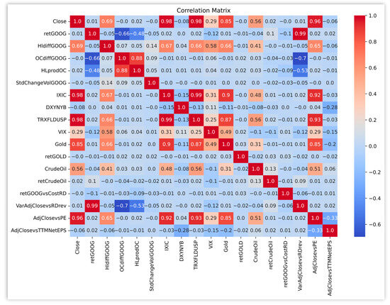
Figure 1.
Correlation among feature variables. Source: Yahoo Finance and Bloomberg.
From Figure 1, note that the target variable, Alphabet’s Close Price, has a high correlation (0.98) with IXIC (Nasdaq Composite Index) and with TRXFLDUSP (Bloomberg U.S. Dollar Total Return Index), but also with gold Close price (0.85), the difference between high and low (0.69) and the crude oil Close price (0.56).
Figure 1 also underlines the strong collinearity among the explanatory variables. The presence of multicollinearity may reduce predictive accuracy, and the interpretability of the models. To improve interpretability, in this paper we have subdivided the collected data into three data sets, which differ by the contained features. The first dataset contains only the lags from 1 day to 5 days of GOOG’s close price. The second dataset includes both financial market data related to the Google stock price, such as retGOOG and HlfiddGOOG, and variables describing the market context in which Alphabet works, such as retGOLD, retCrudeOil, DXYNYB and VIX. The third dataset includes data from annual financial reports, such as retGOOGvsCostRD, VarAdjClosevsRDrev and AdjClosevsTTMNetEPS. All datasets include also the lagged stock price data. In this way, as we moved from the first dataset to the third, we could assess the additional (structural) importance of groups of variables: stock market variables, context variables and report variables.
4. Results
In this section, we compare the performance of the proposed models on the three built datasets. The results of the models, applied to all variables, are shown in Table 2.
Table 2.
Model comparison using all variables.
Table 2 shows that the Long-Short Term model (LSTM), is the most accurate model, as it reaches the lowest MSE, RMSE, MAE and MAPE, as well as the highest R-squared, in the test set. This, however, is not the best fit model in the training set.
4.1. LSTM
We then applied the LSTM model separately to each of the three datasets. The results are reported in Table 3.
Table 3.
Accuracy of Long-Short Term models.
From Table 3, it is possible to note a decline in the results of the LSTM going from the first to the third dataset. We remark that the decrease in accuracy may be compensated by an improvement of explainability and robustness. To understand whether this is true, we present the application of the S.A.F.E. AI metrics, based on the unifying concept of Lorenz inequality, in Table 4, for the LSTM model.
Table 4.
SAFE AI metrics for LSTM models.
From Table 4, it appears that the second dataset shows the highest total explainability. Connecting Table 3 with Table 4, this means that the high accuracy of the LSTM for the first database mainly derives from the lagged price variables, whereas the second database gives a more structural explanation. Finally, note that the LSTM model has a similar robustness across all datasets.
4.2. ANN
We then repeated the detailed analysis performed for the LSTM for the ANN model, the second in performance, as shown in Table 2. We applied the LSTM model separately to each of the three datasets. The results are reported in Table 5.
Table 5.
Accuracy of ANN models.
From Table 5, note that the ANN model performs best in predictive accuracy on the first dataset, similarly to the LSTM model. The worst performance occurs for the second dataset. We now consider the application of the S.A.F.E. AI metrics in Table 6.
Table 6.
Safe AI metrics for ANN models.
From Table 6, note that all models have very low explainability and robustness as, in ANN, lagged variables prevail. In the case of the second dataset, the metrics are equal to zero. A possible strategy to improve the performance of the ANN for the dataset is to reduce the number of lags, possibly reducing them to one. A possible exception is dataset 3, which provides about 10% explanation, which is highly robust. The low RGR results underline the fact that, in a possibly evolving environment, the results of ANN will dramatically change.
4.3. XG Boost
We now consider the XG Boost model in Table 7.
Table 7.
Accuracy of XG Boost models.
From Table 7, the XG Boost model shows, in line with previous models, that the model performed best on dataset1, followed by dataset2 and dataset3. The most explainable features in the second datasets were IXIC and DXYNYB (0.5581 and 0.0273) while in the third one, the most explainable features were IXIC, Crude Oil price and retGOOG, respectively, 0.1921, 0.0279 and 0.0199.
We now consider the application of the S.A.F.E. AI metrics in Table 8.
Table 8.
Safe AI metrics for XG Boost model.
The S.A.F.E. AI metrics in Table 8 denote generally good accuracy but a big difference with respect to explainability. The second dataset is the most explainable, in line with the result from the LSTM model. The main issue concerning this model is the overall robustness when perturbing data with small values of RGR.
4.4. Ridge Linear Regression
We finally consider the Ridge regression model in Table 9.
Table 9.
Accuracy of Ridge regression model.
Table 9 shows a result in line with the previous models: the model is more accurate for the first database, followed by the second and the third. The S.A.F.E. AI metrics are shown in Table 10.
Table 10.
Safe AI metrics for the Ridge regression model.
The S.A.F.E. AI metrics in Table 10 denote good accuracy but low explainability. The second dataset is the most explainable, in line with the result from the previous model. The robustness is high, as we expect from this type of model.
5. Concluding Remarks
Our aim was to predict Alphabet’s stock price, taking into consideration the possible explanatory factors. To achieve this goal, we built three different datasets, considering autoregressive financial market data (dataset1), economic context data (dataset2) and company financial report data (dataset3).
We then compared four machine learning models for the three considered datasets. The models were compared not only in terms of predictive accuracy, but also in terms of robustness and explainability, in line with the recently proposed S.A.F.E. AI approach.
Our findings underscore the importance of careful model selection in light of the desired outcomes. If the primary goal is predictive accuracy, all of the models show acceptable RGA values, ranging from 0.9625 to 0.9955. If the focus is instead on robustness, the Ridge regression model seems to be the most suitable choice, together with LSTM. If explainability is prioritized over robustness, XG Boost will be the best choice.
The trade-off between all those aspects should guide the choice of the model, depending on the specific application and goals. Alternatively, the value of each metric can be mapped onto a probability, and the three resulting probabilities can be multiplied together. This led, in the case of Dataset2, to a probability of about 0.38 for LSTM, 0.19 for XGboost and 0.33 for Ridge, indicating that the LSTM is the model with the highest probability of being safe, in this case.
More generally, taking into account also data comparison, if the focus is mainly in obtaining a high predictive accuracy, a user should consider an LSTM model, possibly using the first dataset. If the focus is mainly on obtaining a model which is easier to explain and understand, a user should consider XGBOOST, possibly using the third dataset. If the focus is on obtaining a model that is robust to data perturbations and outliers, a user should consider Ridge linear regression for one of the three datasets.
From a financial management practice, the paper indicates how stock price can be predicted using several independent variables, with their lagged values.
Future research may consider hybrid models integrating LSTM, XGBOOST and RIDGE to jointly improve explainability, robustness and accuracy and/or add further variables, such as technical analysis indicators.
Additionally, the work can be extended to predict other stock prices, and, possibly, to use Google stock prices to predict other stock prices.
Author Contributions
Conceptualization, P.G.; methodology, P.G.; software, C.E.B.; validation, P.G.; formal analysis, C.E.B.; investigation, C.E.B.; resources, P.G.; data curation, C.E.B.; writing—original draft preparation, C.E.B.; writing—review and editing, C.E.B.; visualization, C.E.B.; supervision, P.G.; project administration, P.G.; no funding acquisition. All authors have read and agreed to the published version of the manuscript.
Funding
This research received no external funding.
Data Availability Statement
The raw data supporting the conclusions of this article will be made available by the authors on request.
Conflicts of Interest
The authors declare no conflict of interest.
References
- Babaei, G.; Giudici, P.; Raffinetti, E. A Rank graduation box for SAFE Artificial Intelligence. Expert Syst. Appl. 2025, 29, 125329. [Google Scholar] [CrossRef]
- James, G.; Witten, D.; Hastie, T.; Tibshirani, R. An Introduction to Statistical Learning with Applications in R, Second Edition. 2021. Available online: https://www.statlearning.com/ (accessed on 19 July 2024).
- Miller, A.; Panneerselvam, J.; Liu, L. A review of regression and classification techniques for analysis of common and rare variants and gene-environmental factors. Neurocomputing 2022, 489, 466–485. [Google Scholar] [CrossRef]
- Pereira, J.M.; Basto, M.; Ferreira da Silva, A. The Logistic Lasso and Ridge Regression in Predicting Corporate Failure. Procedia Econ. Financ. 2016, 39, 634–641. [Google Scholar] [CrossRef]
- Chen, T.; Guestrin, C. XGBoost: A Scalable Tree Boosting System; Association for Computing Machinery: New York, NY, USA, 2016; pp. 785–794. [Google Scholar] [CrossRef]
- Tarwidi, D.; Pudjaprasetya, S.R.; Adytia, D.; Apri, M. An optimized XGBoost-based machine learning method for predicting wave run-up on a sloping beach. MethodsX 2023, 10, 102119. [Google Scholar] [CrossRef] [PubMed]
- Maind, B.; Wankar, P. Basics of Artificial Neural Network. Int. J. Recent Innov. Trends Comput. Commun. 2014, 2, 96–100. [Google Scholar] [CrossRef]
- Vasileiadis, A.; Alexandrou, E.; Paschalidou, L. Artificial Neural Networks and Its Applications. arXiv 2024, arXiv:2110.09021. [Google Scholar] [CrossRef]
- Van Houdt, G.; Mosquera, C.; Nápoles, G. A Review on the Long Short-Term Memory Model. Artif. Intell. Rev. 2020, 53, 5929–5955. [Google Scholar] [CrossRef]
- Sherstinsky, A. Fundamentals of Recurrent Neural Network (RNN) and Long Short-Term Memory (LSTM) network. Phys. D Nonlinear Phenom. 2020, 404, 132306. [Google Scholar] [CrossRef]
Disclaimer/Publisher’s Note: The statements, opinions and data contained in all publications are solely those of the individual author(s) and contributor(s) and not of MDPI and/or the editor(s). MDPI and/or the editor(s) disclaim responsibility for any injury to people or property resulting from any ideas, methods, instructions or products referred to in the content. |
© 2025 by the authors. Licensee MDPI, Basel, Switzerland. This article is an open access article distributed under the terms and conditions of the Creative Commons Attribution (CC BY) license (https://creativecommons.org/licenses/by/4.0/).