

Analytical MPC Algorithm Using Steady-State Process Model


Abstract
1. Introduction
2. Materials and Methods
2.1. MPC Algorithms
2.2. Analytical DMC Algorithm
2.3. Efficient SSDMC Algorithm
3. Results
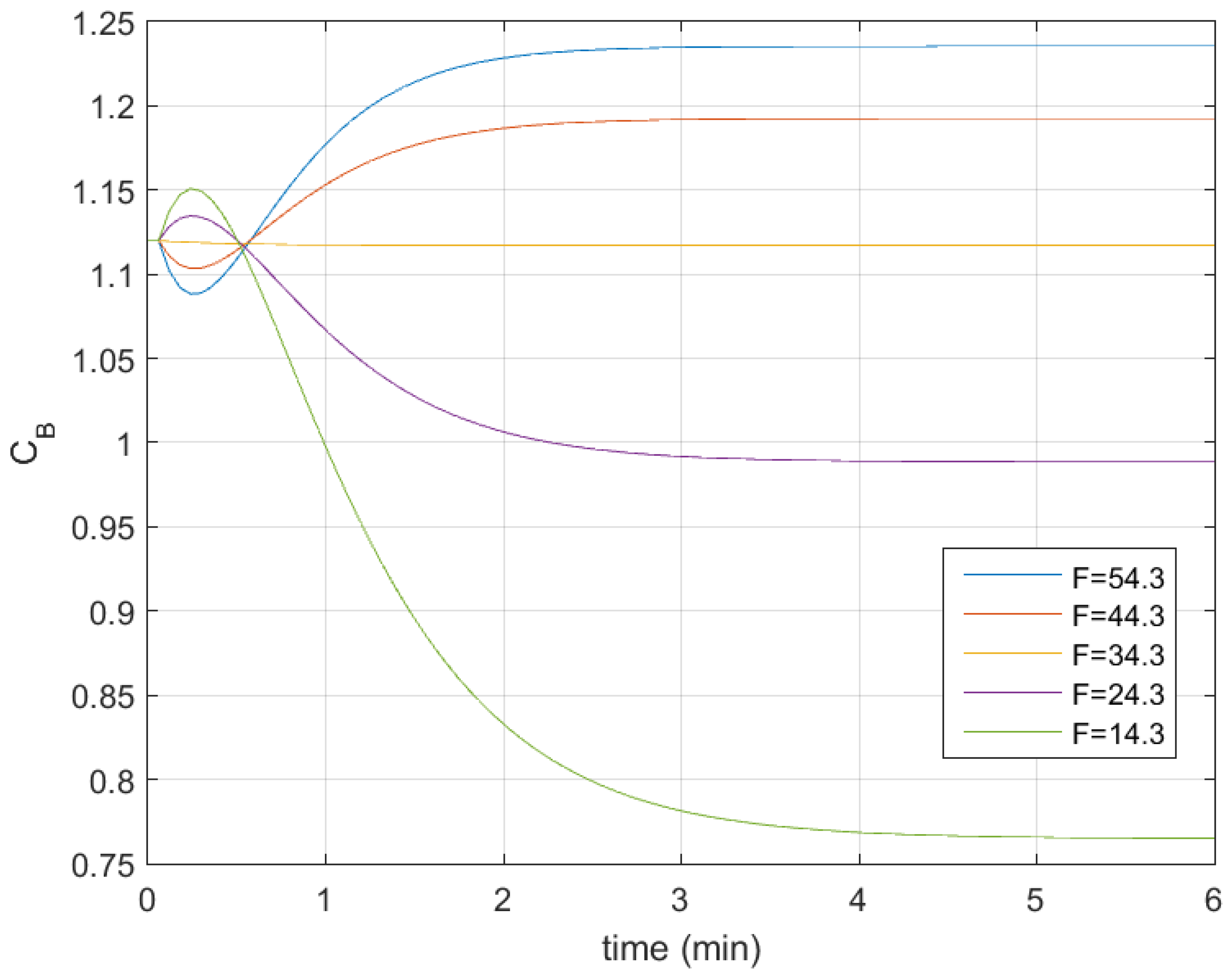
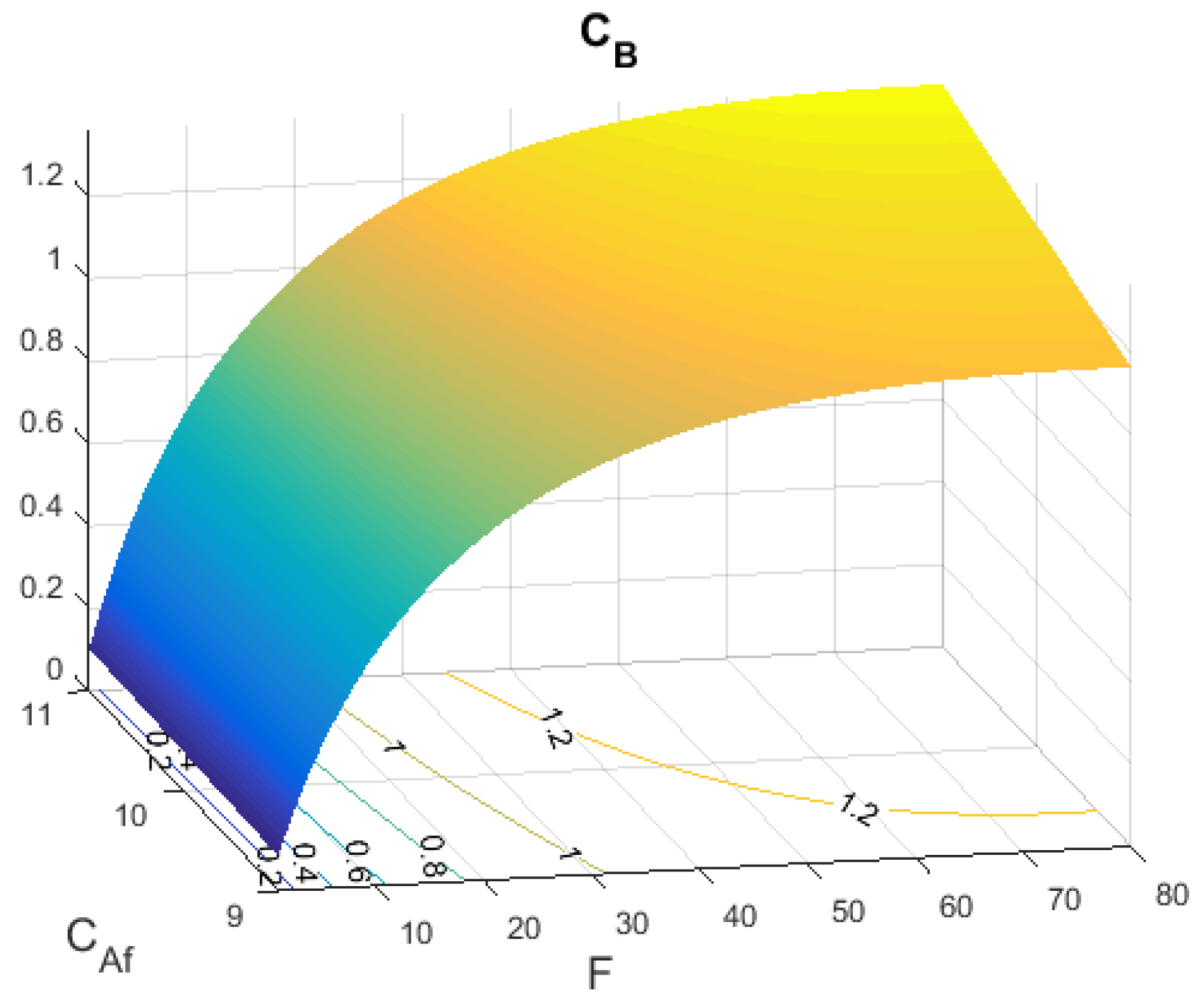
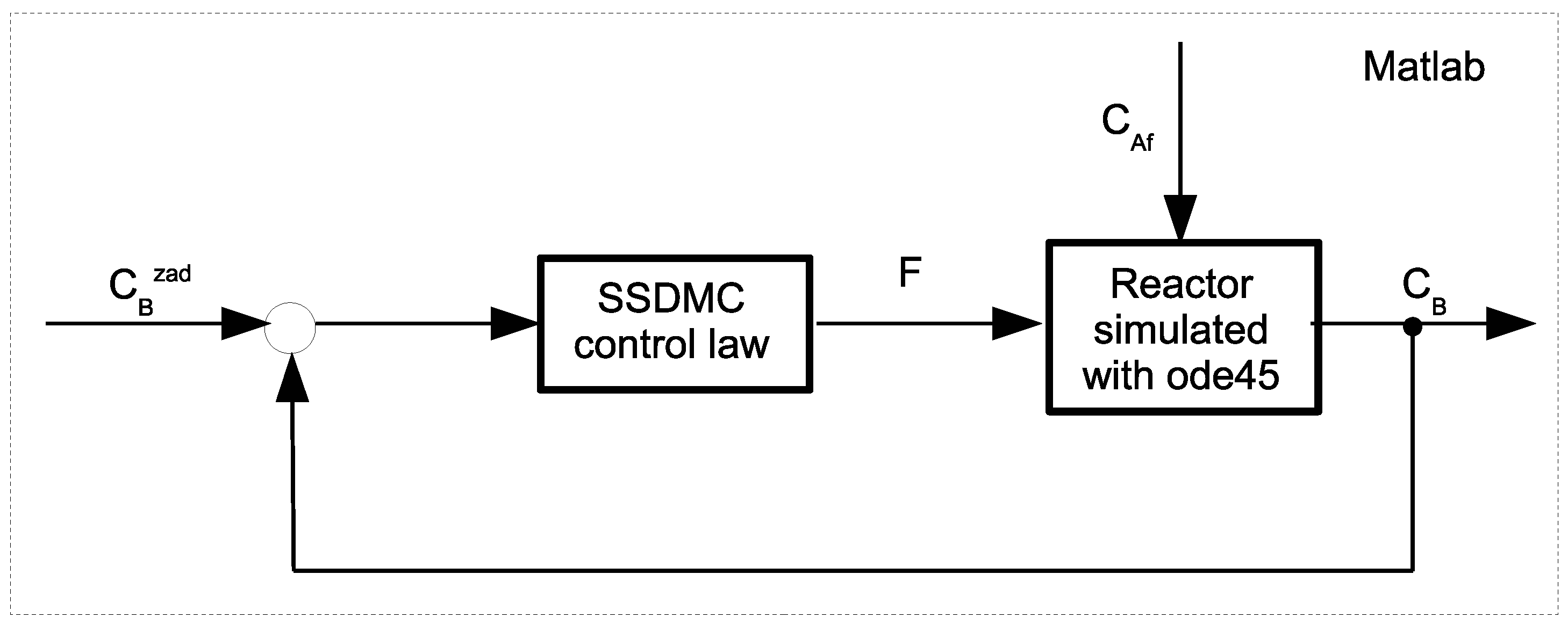
3.1. Control Plant
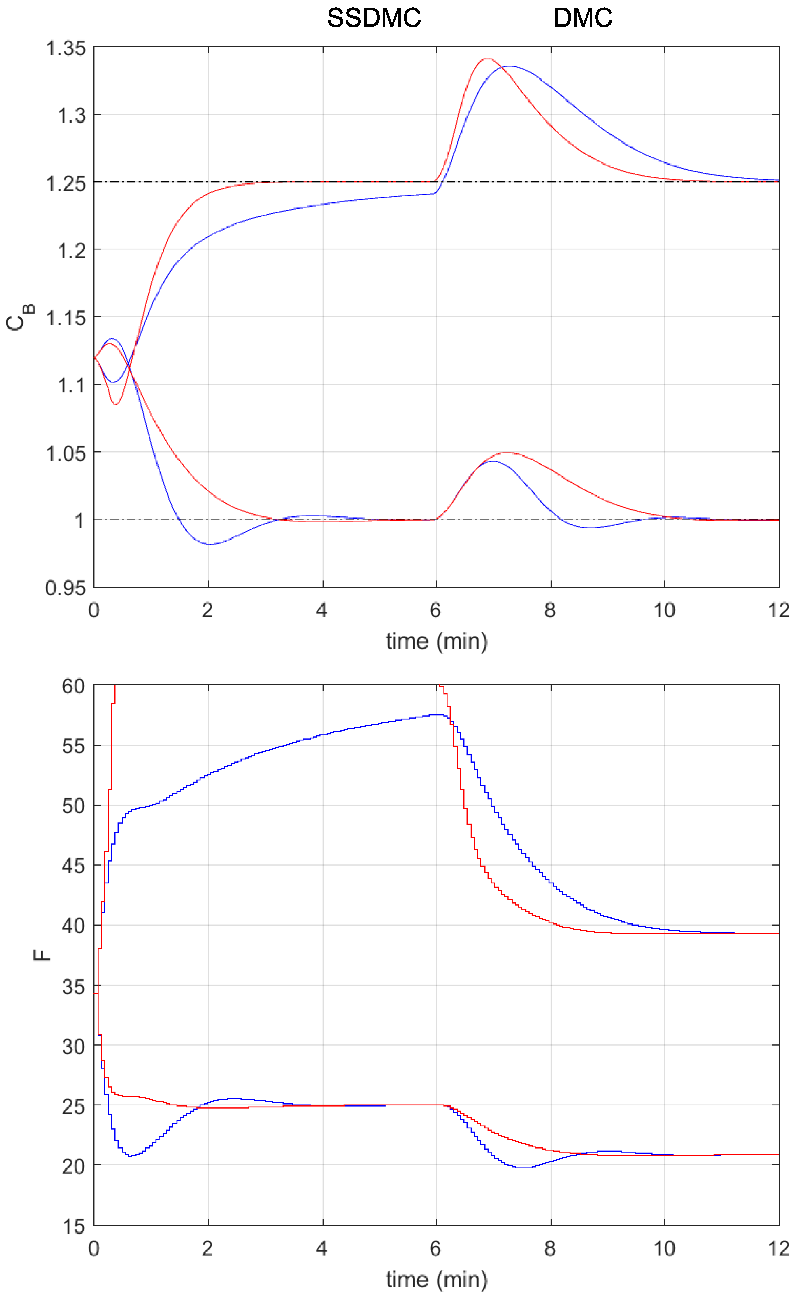
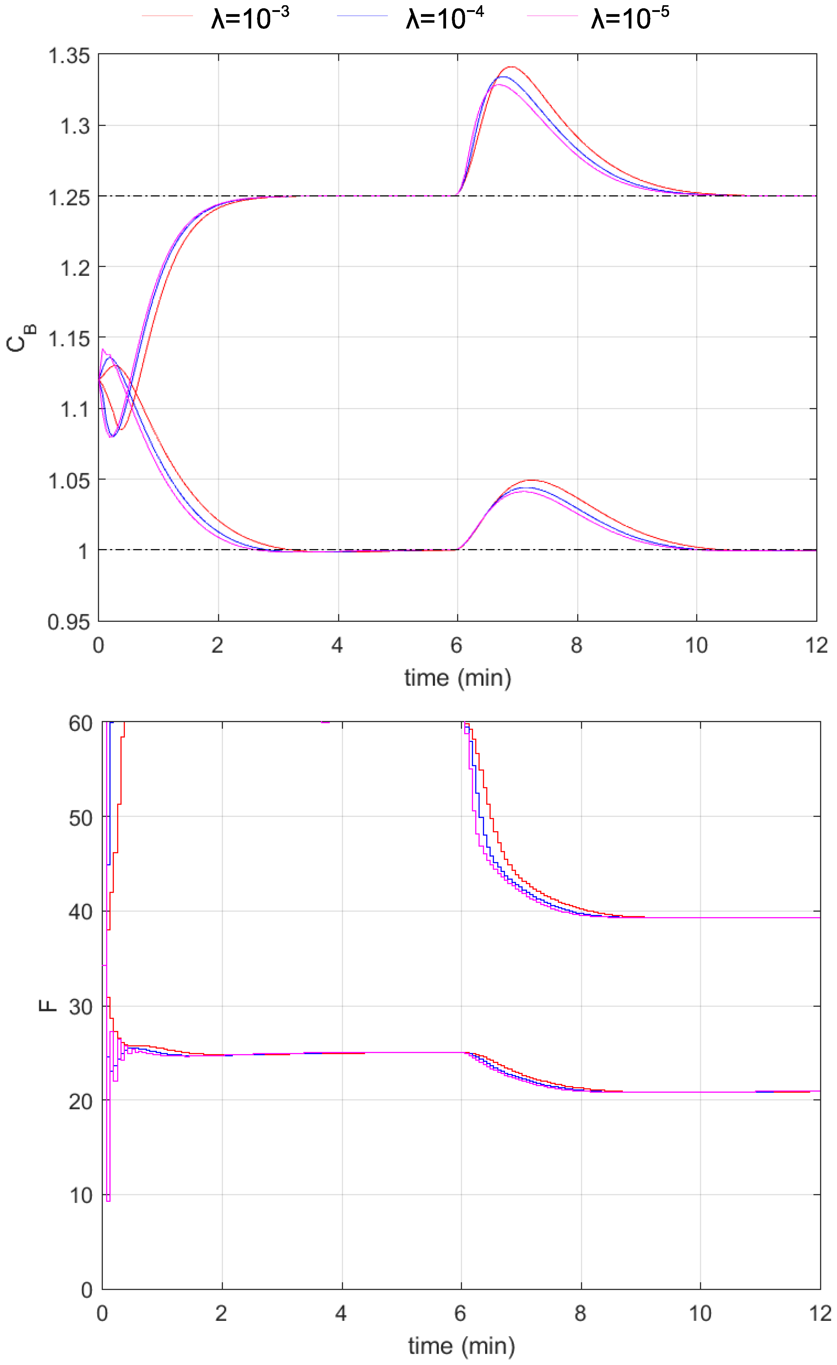
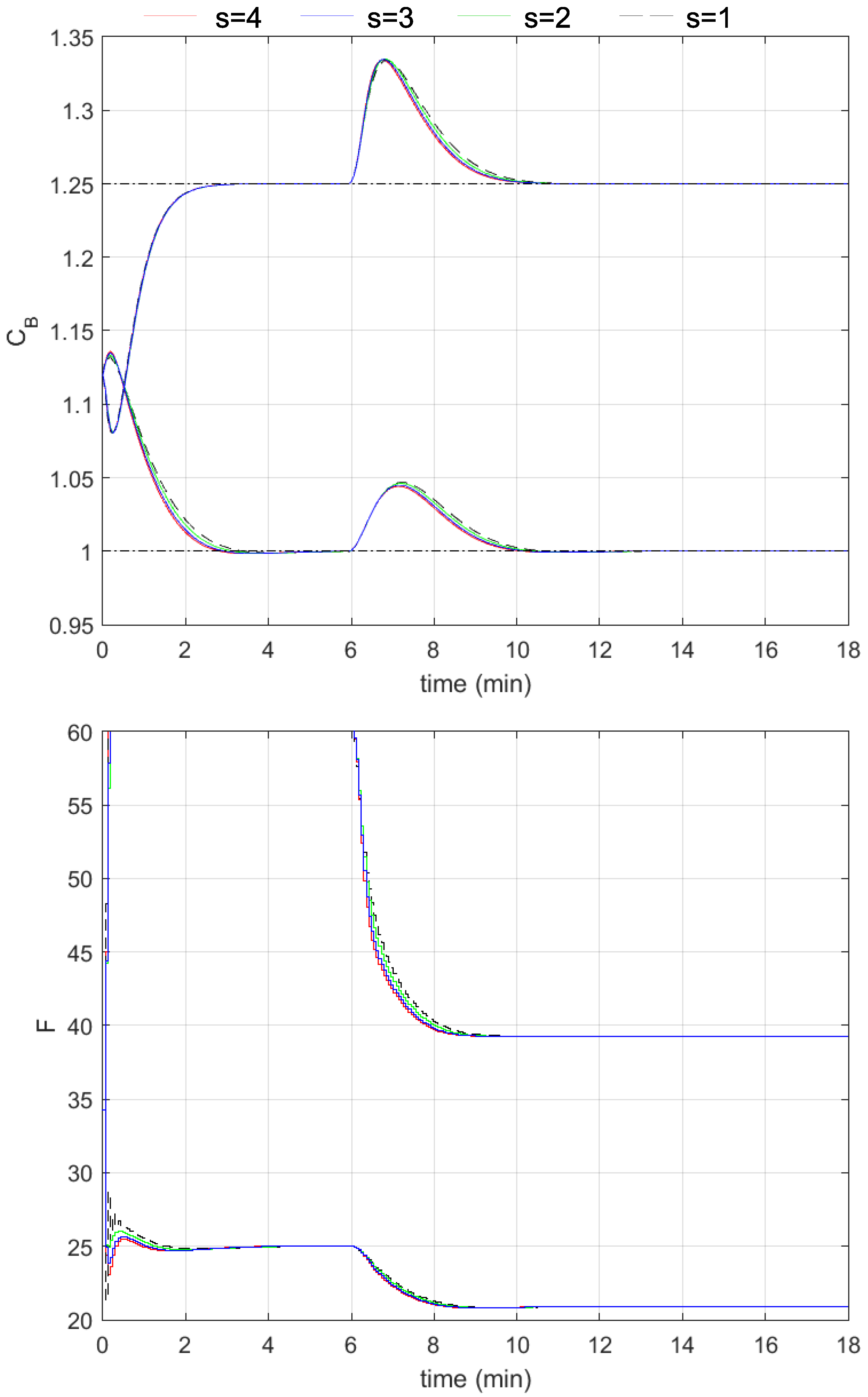
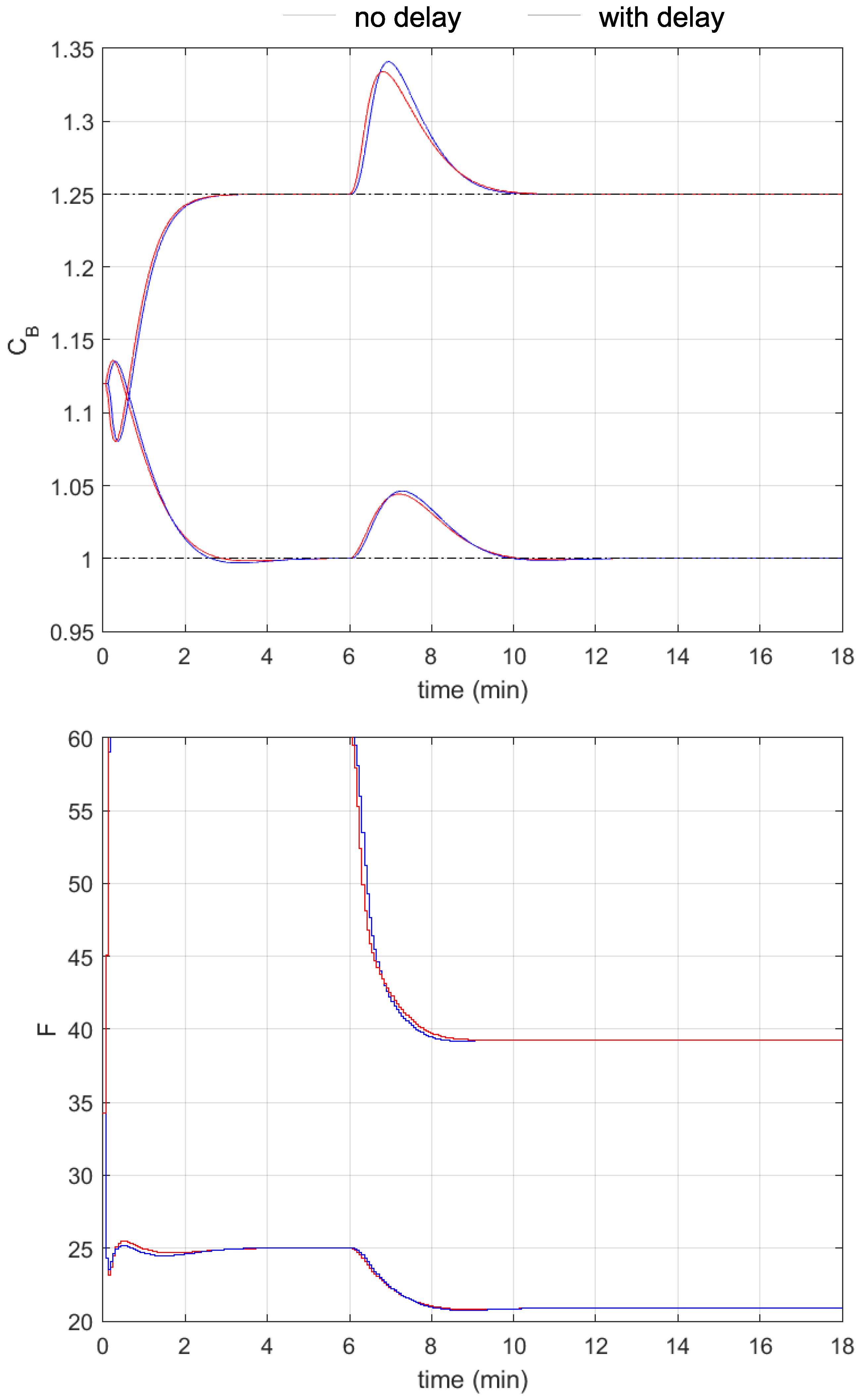
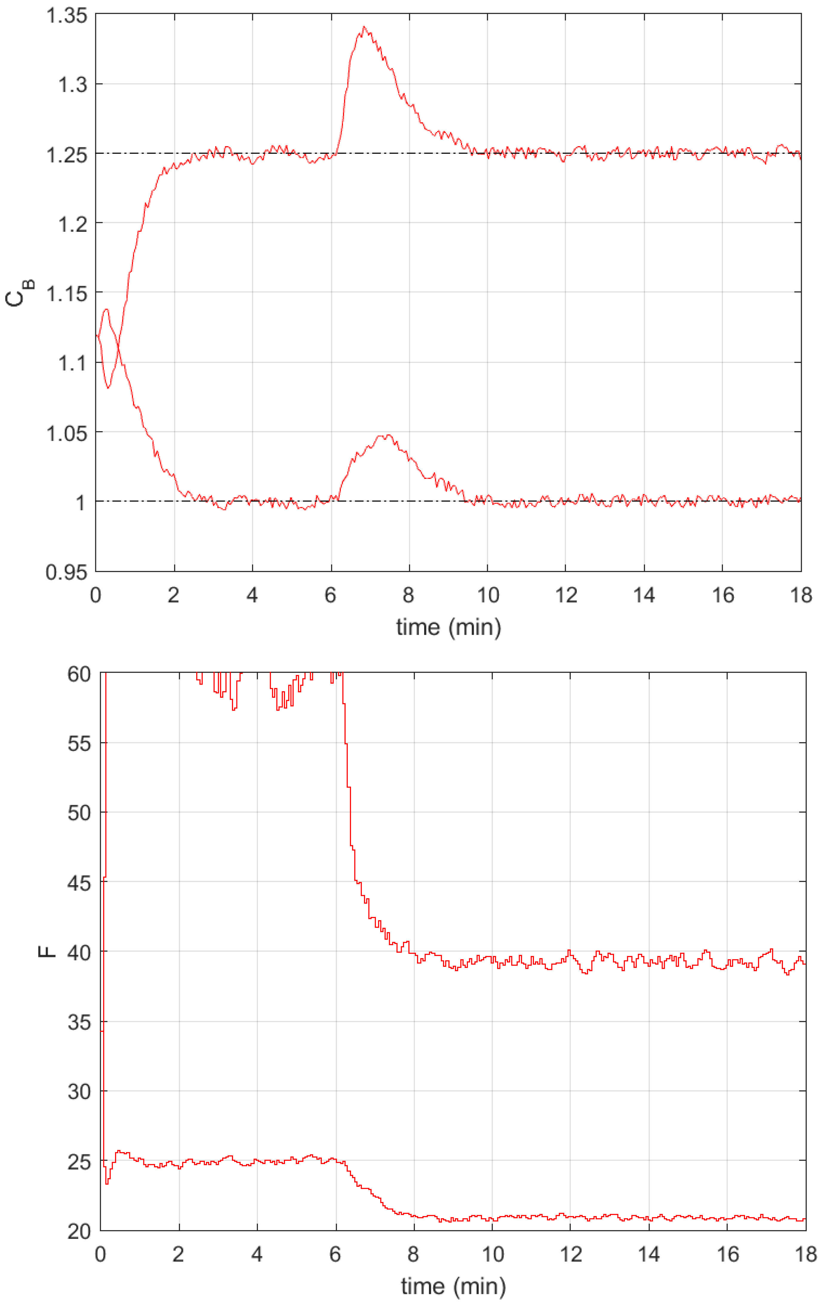
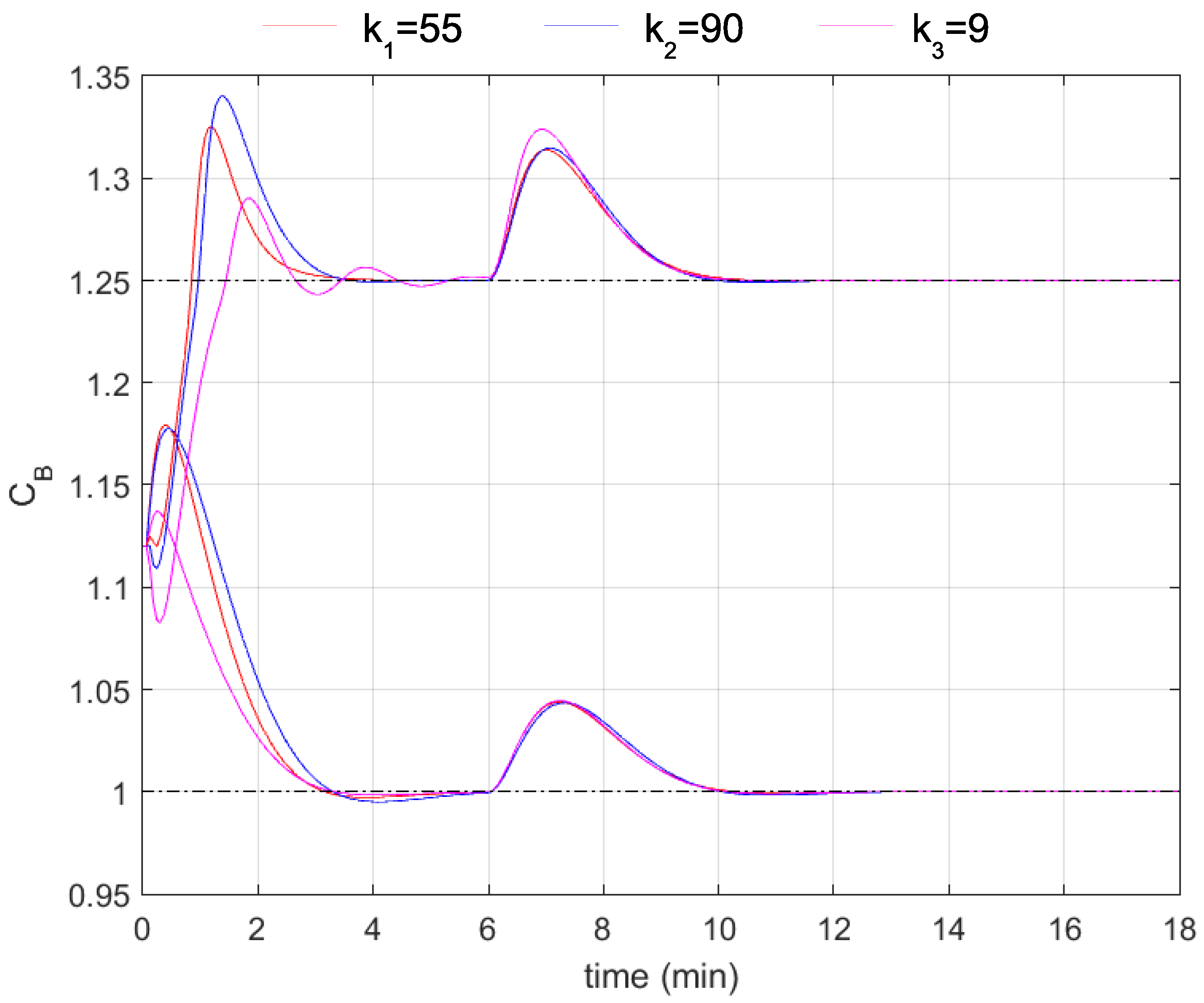
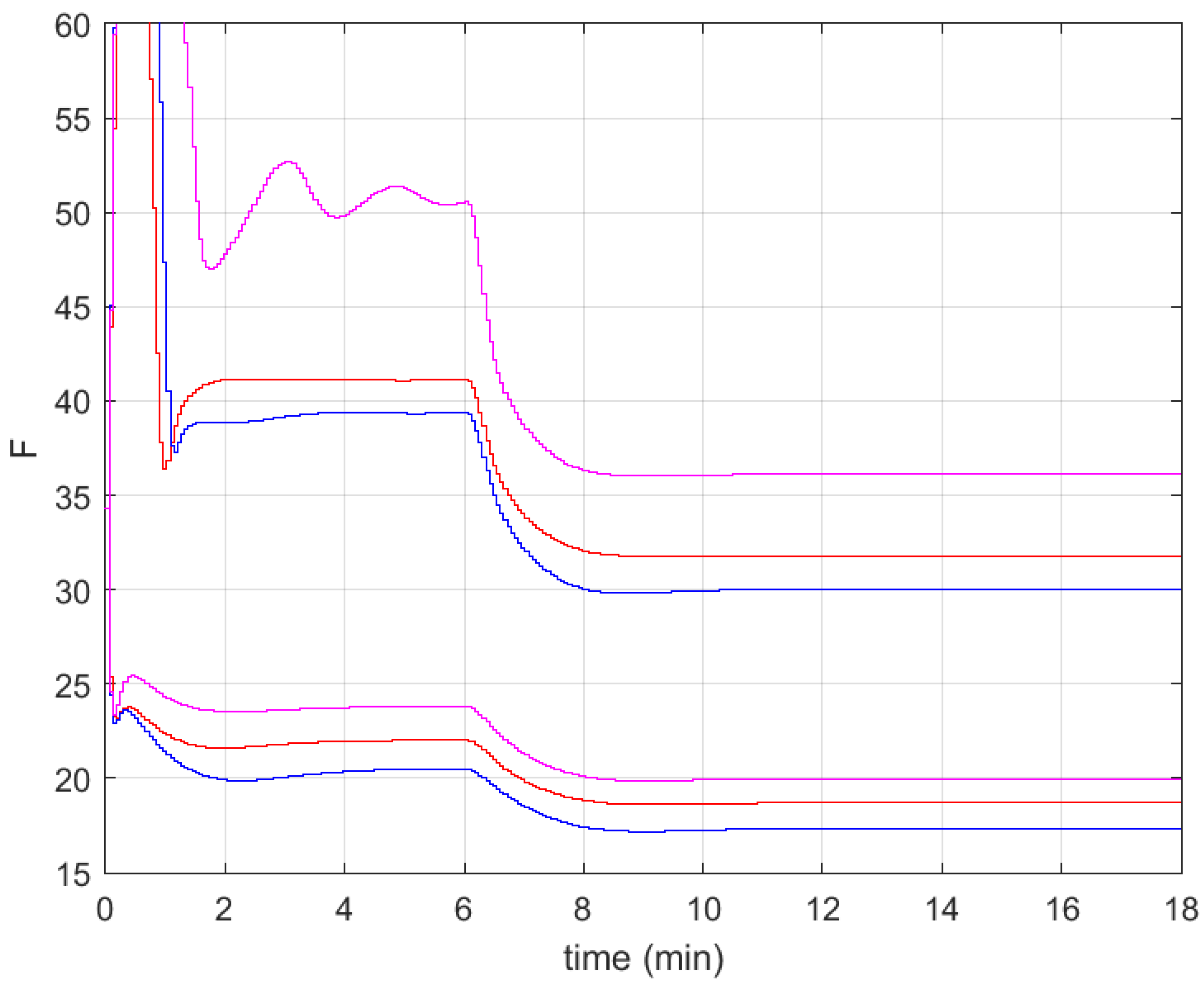
3.2. Simulation Results
4. Discussion and Conclusions
Funding
Data Availability Statement
Conflicts of Interest
Abbreviations
| CSTR | Continuous Stirred-Tank Reactor |
| DMC | Dynamic Matrix Control |
| LMI | Linear Matrix Inequality |
| LMPC | Linear Model-Based Model Predictive Control |
| MPC | Model Predictive Control |
| NMPC | Nonlinear Model-Based MPC |
| PID | Proportional–Integral–Derivative |
| SISO | Single-Input Single-Output |
| SSDMC | Steady-State Model-Based Dynamic Matrix Control |
References
- Arteaga, M.A.; Guajardo-Benavides, E.J.; Sánchez-Sánchez, P. Stability Analysis and Experimental Validation of Standard Proportional-Integral-Derivative Control in Bilateral Teleoperators with Time-Varying Delays. Algorithms 2024, 17, 580. [Google Scholar] [CrossRef]
- Candan, F.; Dik, O.F.; Kumbasar, T.; Mahfouf, M.; Mihaylova, L. Real-Time Interval Type-2 Fuzzy Control of an Unmanned Aerial Vehicle with Flexible Cable-Connected Payload. Algorithms 2023, 16, 273. [Google Scholar] [CrossRef]
- Kong, W.; Zhang, H.; Yang, X.; Yao, Z.; Wang, R.; Yang, W.; Zhang, J. PID control algorithm based on multistrategy enhanced dung beetle optimizer and back propagation neural network for DC motor control. Sci. Rep. 2024, 14, 28276. [Google Scholar] [CrossRef]
- Mao, W.-L.; Chen, S.-H.; Kao, C.-Y. Fractional-Order Fuzzy PID Controller with Evolutionary Computation for an Effective Synchronized Gantry System. Algorithms 2024, 17, 58. [Google Scholar] [CrossRef]
- Guo, X.; Shirkhani, M.; Ahmed, E.M. Machine-Learning-Based Improved Smith Predictive Control for MIMO Processes. Mathematics 2022, 10, 3696. [Google Scholar] [CrossRef]
- Mohammadzaheri, G.M.; Ghodsi, M. An Enhanced Smith-Predictor-based Control System for delayed MIMO Processes and its Use on a CSTR with Multiple Time-delays. In Proceedings of the 2023 28th International Conference on Automation and Computing (ICAC), Birmingham, UK, 30 August–1 September 2023; pp. 1–6. [Google Scholar]
- Camacho, E.F.; Bordons, C. Model Predictive Control; Springer: London, UK, 1999. [Google Scholar]
- Maciejowski, J.M. Predictive Control with Constraints; Prentice Hall: Harlow, UK, 2002. [Google Scholar]
- Nebeluk, R.; Marusak, P. Efficient MPC algorithms with variable trajectories of parameters weighting predicted control errors. Arch. Control Sci. 2020, 30, 325–363. [Google Scholar]
- Rossiter, J.A. Model–Based Predictive Control: A Practical Approach; CRC Press: Boca Raton, FL, USA, 2003. [Google Scholar]
- Sands, T. Comparison and Interpretation Methods for Predictive Control of Mechanics. Algorithms 2019, 12, 232. [Google Scholar] [CrossRef]
- Tatjewski, P. Advanced Control of Industrial Processes; Structures and Algorithms; Springer: London, UK, 2007. [Google Scholar]
- Ławryńczuk, M. Computationally Efficient Model Predictive Control Algorithms: A Neural Network Approach; Springer: Berlin/Heidelberg, Germany, 2014. [Google Scholar]
- Mohamed, M.A.-E.-H.; Abbas, H.S.; Shouran, M.; Kamel, S. A Neuro-Predictive Controller Scheme for Integration of a Basic Wind Energy Generation Unit with an Electrical Power System. Energies 2022, 15, 5839. [Google Scholar] [CrossRef]
- Mohammadzaheri, M.; Chen, L.; Mirsepahi, A.; Ghanbari, M.; Tafreshi, R. Neuro-Predictive Control of an Infrared Dryer with a Feedforward-Feedback Approach. Asian J. Control 2015, 17, 1972–1977. [Google Scholar] [CrossRef]
- Abdelaal, M.; Schön, S. Predictive Path Following and Collision Avoidance of Autonomous Connected Vehicles. Algorithms 2020, 13, 52. [Google Scholar] [CrossRef]
- Chen, H.; Allgöwer, F. A Quasi-Infinite Horizon Nonlinear Model Predictive Control Scheme with Guaranteed Stability. Automatica 1998, 34, 1205–1217. [Google Scholar] [CrossRef]
- Tatjewski, P. Offset–free nonlinear model predictive control with state–space process models. Arch. Control Sci. 2017, 27, 595–615. [Google Scholar] [CrossRef]
- Diehl, M.; Bock, H.G.; Schlöder, J.P.; Findeisen, R.; Nagy, Z.; Allgöwer, F. Real–time optimization and nonlinear model predictive control of processes governed by differential–algebraic equations. J. Process Control 2002, 12, 577–585. [Google Scholar] [CrossRef]
- Schäfer, A.; Kühl, P.; Diehl, M.; Schlöder, J.; Bock, H.G. Fast reduced multiple shooting methods for nonlinear model predictive control. Chem. Eng. Process. 2007, 46, 1200–1214. [Google Scholar] [CrossRef]
- Zavala, V.M.; Laird, C.D.; Biegler, L.T. A fast moving horizon estimation algorithm based on nonlinear programming sensitivity. J. Process Control 2008, 18, 876–884. [Google Scholar] [CrossRef]
- Ławryńczuk, M. Nonlinear state–space predictive control with on–line linearisation and state estimation. Int. J. Appl. Math. Comput. Sci. 2015, 25, 833–847. [Google Scholar] [CrossRef]
- Morari, M.; Lee, J.H. Model predictive control: Past, present and future. Comput. Chem. Eng. 1999, 23, 667–682. [Google Scholar] [CrossRef]
- Marusak, P. Efficient model predictive control algorithm with fuzzy approximations of nonlinear models. LNCS 2009, 5495, 448–457. [Google Scholar]
- Marusak, P. Advantages of an easy to design fuzzy predictive algorithm in control systems of nonlinear chemical reactors. Appl. Soft Comput. 2009, 9, 1111–1125. [Google Scholar] [CrossRef]
- Marusak, P. Numerically Efficient Fuzzy MPC Algorithm with Advanced Generation of Prediction: Application to a Chemical Reactor. Algorithms 2020, 13, 143. [Google Scholar] [CrossRef]
- Marusak, P. Advanced Construction of Dynamic Matrix in Numerically Efficient Fuzzy MPC Algorithms. Algorithms 2021, 14, 25. [Google Scholar] [CrossRef]
- Nebeluk, R.; Ławryńczuk, M. Fast Nonlinear Predictive Control Using Classical and Parallel Wiener Models: A Comparison for a Neutralization Reactor Process. Sensors 2023, 23, 9539. [Google Scholar] [CrossRef]
- Dominguez, L.F.; Pistikopoulos, E.N. A Novel mp-NLP Algorithm for Explicit/Multi-parametric NMPC. In Proceedings of the 8th IFAC Symposium on Nonlinear Control Systems, Bologna, Italy, 1–3 September 2010. [Google Scholar]
- Johansen, T.A. On multi–parametric nonlinear programming and explicit nonlinear model predictive control. In Proceedings of the 41st IEEE Conf Decision and Control, Las Vegas, NV, USA, 10–13 December 2002; Volume 3, pp. 2768–2773. [Google Scholar]
- Johansen, T.A. Approximate explicit receding horizon control of constrained nonlinear systems. Automatica 2004, 40, 293–300. [Google Scholar] [CrossRef]
- Bemporad, A.; Borrelli, F.; Morari, M. Piecewise linear optimal controllers for hybrid systems. In Proceedings of the 2000 American Control Conference, Chicago, IL, USA, 28–30 June 2000; Volume 2, pp. 1190–1194. [Google Scholar]
- Bemporad, A.; Morari, M.; Dua, V.; Pistikopoulos, E.N. The explicit linear quadratic regulator for constrained systems. Automatica 2002, 38, 3–20. [Google Scholar] [CrossRef]
- Pistikopoulos, E.N.; Dua, V.; Bozinis, N.A.; Bemporad, A.; Morari, M. On–line optimization via off–line parametric optimization tools. Comput. Chem. Eng. 2002, 26, 175–185. [Google Scholar] [CrossRef]
- Chaber, P.; Ławryńczuk, M. Fast analytical model predictive controllers and their implementation for STM32 ARMmicrocontroller. IEEE Trans. Ind. Inform. 2019, 15, 4580–4590. [Google Scholar] [CrossRef]
- Wojtulewicz, A.; Ławryńczuk, M. Implementation of multiple–input multiple–output dynamic matrix control algorithm for fast processes using field programmable gate array. IFAC–PapersOnLine 2018, 51, 324–329. [Google Scholar] [CrossRef]
- Bagheri, P.; Sedigh, A.K. Analytical approach to tuning of model predictive control for first-order plus dead time models. IET Control Theory Appl. 2013, 7, 1806–1817. [Google Scholar] [CrossRef]
- Short, M. Move suppression calculations for well-conditioned MPC. ISA Trans. 2017, 67, 371–381. [Google Scholar] [CrossRef]
- Zheng, H.; Zou, T.; Hu, J.; Yu, H. An offline optimization and online table look-up strategy of two-layer model predictive control. IEEE Access 2018, 6, 47433–47441. [Google Scholar] [CrossRef]
- Abbas, H.S.; Hanema, J.; Tóth, R.; Mohammadpour, J.; Meskin, N. An improved robust model predictive control for linear parameter-varying input-output models. Int. J. Robust Nonlinear Control 2018, 28, 859–880. [Google Scholar] [CrossRef]
- Ding, B.; Zou, T. A synthesis approach for output feedback robust model predictive control based-on input–output model. J. Process Control 2014, 24, 60–72. [Google Scholar] [CrossRef]
- Yan, Y.; Zhang, L. Robust Model Predictive Control with Almost Zero Online Computation. Mathematics 2021, 9, 242. [Google Scholar] [CrossRef]
- Marusak, P. A numerically efficient fuzzy MPC algorithm with fast generation of the control signal. Int. J. Appl. Math. Comput. Sci. 2021, 31, 59–71. [Google Scholar] [CrossRef]
- Jain, A.; Taparia, R. Laguerre function based model predictive control for van–de–vusse reactor. In Proceedings of the 2nd IEEE International Conference on Power Electronics, Intelligent Control and Energy Systems, ICPEICES 2018, Delhi, India, 22–24 October 2018; Volume 3, pp. 1010–1015. [Google Scholar]
- Mate, S.; Kodamana, H.; Bhartiya, S.; Nataraj, P.S.V. A Stabilizing Sub–Optimal Model Predictive Control for Quasi–Linear Parameter Varying Systems. IEEE Control Syst. Lett. 2020, 4, 402–407. [Google Scholar] [CrossRef]
- Ribeiro, L.M.; Secchi, A.R. A methodology to obtain analytical models that reduce the computational complexity faced in real time implementation of NMPC controllers. Braz. J. Chem. Eng. 2019, 36, 1255–1277. [Google Scholar] [CrossRef]
- Nguyen, T.S.; Hoang, N.H.; Hussain, M.A. Tracking error plus damping injection control of non-minimum phase processes. IFAC-Papers Online 2018, 51, 643–648. [Google Scholar] [CrossRef]
- Uçak, K. A Runge–Kutta neural network-based control method for nonlinear MIMO systems. Soft Comput. 2019, 23, 7769–7803. [Google Scholar] [CrossRef]
- Uçak, K. A Novel Model Predictive Runge–Kutta Neural Network Controller for Nonlinear MIMO Systems. Neural Process. Lett. 2020, 51, 1789–1833. [Google Scholar] [CrossRef]
- Banerjee, S.; Khan, O.; El Mistiri, M.; Nandola, N.N.; Rivera, D.E. Data-Driven Control of Highly Interactive Systems using 3DoF Model-On-Demand MPC: Application to a MIMO CSTR. IFAC-PapersOnLine 2024, 58, 420–425. [Google Scholar] [CrossRef]
- Mohammadzaheri, M.; Chen, L. Double-command fuzzy control of a nonlinear CSTR. Korean J. Chem. Eng 2010, 27, 19–31. [Google Scholar] [CrossRef]
- Doyle, F.; Ogunnaike, B.A.; Pearson, R.K. Nonlinear model–based control using second–order Volterra models. Automatica 1995, 31, 697–714. [Google Scholar] [CrossRef]
Disclaimer/Publisher’s Note: The statements, opinions and data contained in all publications are solely those of the individual author(s) and contributor(s) and not of MDPI and/or the editor(s). MDPI and/or the editor(s) disclaim responsibility for any injury to people or property resulting from any ideas, methods, instructions or products referred to in the content. |
© 2025 by the author. Licensee MDPI, Basel, Switzerland. This article is an open access article distributed under the terms and conditions of the Creative Commons Attribution (CC BY) license (https://creativecommons.org/licenses/by/4.0/).
Share and Cite
Marusak, P.M. Analytical MPC Algorithm Using Steady-State Process Model. Algorithms 2025, 18, 79. https://doi.org/10.3390/a18020079
Marusak PM. Analytical MPC Algorithm Using Steady-State Process Model. Algorithms. 2025; 18(2):79. https://doi.org/10.3390/a18020079
Chicago/Turabian StyleMarusak, Piotr M. 2025. "Analytical MPC Algorithm Using Steady-State Process Model" Algorithms 18, no. 2: 79. https://doi.org/10.3390/a18020079
APA StyleMarusak, P. M. (2025). Analytical MPC Algorithm Using Steady-State Process Model. Algorithms, 18(2), 79. https://doi.org/10.3390/a18020079