SA-Net: Leveraging Spatial Correlations Spatial-Aware Net for Multi-Perspective Robust Estimation Algorithm

Abstract

Robust estimation aims to provide accurate and reliable parameter estimations, particularly when data are affected by noise or outliers. Traditional methods like random sample consensus (RANSAC) struggle with handling outliers because they treat all observations as equally important. A series of advanced deep learning methods have recently emerged, which use deep learning techniques to estimate the probability of each sample being selected, prioritizing higher confidence for observations that are closer to the ground truth model. However, optimizing solely based on proximity to the ground truth model does not guarantee higher-quality estimations. Meanwhile spatial relationships between the data points in the minimum sampled set also influence the accuracy of the final estimated model. To address these issues, we propose Spatial-Aware Net (SA-Net), a dual-branch neural network that integrates both confidence and spatial encodings. SA-Net employs a confidence distribution encoder to learn the confidence distribution and a spatial distribution encoder to capture spatial correlations between point features. By incorporating multi-perspective sampling, the minimum sample set can be selected based on different spatial distributions in the output of the neural network, and applying Chamfer Loss constraints, our approach improves model optimization and effectively mitigates suboptimal solutions. Extensive experiments demonstrate that SA-Net outperforms the state of the art across various real-world robust estimation tasks.

1. Introduction

Robust estimation refers to learning a model parameter for data that have been contaminated by noise and outliers, which is crucial in applications such as motion segmentation [1], pose graph initialization in Structure-from-Motion algorithms [2,3,4], and image mosaicing [5,6,7]. Random sample consensus (RANSAC) facilitates the accurate estimation of model parameters from datasets containing outliers. RANSAC is achieved by iteratively selecting random subsets of observations, called minimal sets, to generate model hypotheses. To assess the quality of the estimations, RANSAC evaluates each model by maximizing its consensus with the entire dataset. Recent approaches, such as marginalizing sample consensus (MAGSAC) [8] and marginalizing sample consensus plus plus (MAGSAC++) [9], further refine this process by scoring models based on a marginalized inlier counting. Deep learning methods adhere to the overall framework of RANSAC, taking data points as input. Through the deep learning network, the probability of each sample being selected for sampling is computed. The Gumbel-Softmax technique is employed to make the probabilistic sampling process differentiable, enabling the identification of the minimum sample set. Subsequently, a model is estimated based on this minimum sample set, yielding the final matrix results. This paper focuses on the application of robust model estimation algorithms in computer vision, specifically using correspondences obtained from pre-processing matching algorithms to estimate the essential matrix and fundamental matrix between stereo views. The essential matrix describes the geometric relationship between two cameras when the intrinsic camera parameters are known, thereby reflecting the mapping relationship between the two coordinate systems. The fundamental matrix, on the other hand, is independent of the camera’s intrinsic parameters and primarily serves to map a point in one image to the corresponding epipolar line in another image.

However, previous methods typically relied on the confidence distribution of data points, using the distance to the ground truth model as a direct optimization objective. However, a shorter distance between the matches in the minimal sets and the ground truth model does not necessarily indicate a higher-quality estimated model [10]. We show an illustration in Figure 1a; the ill-conditioned minimal sets, despite being closer to the ground truth model, lead to worse results than the normal minimal sets in line fitting problems. Meanwhile, Figure 1b also shows the lower inlier ratio of the minimal sets associated with the best model compared with the minimal sets associated with the good model. This suggests that within a certain range of error, the distance from the points to the model should not be the sole criterion for sampling. Despite fine-tuning the neural network with ill-conditioned samples being able to somewhat improve model optimization [10], it only partially addresses the issue from a data perspective, the underlying cause of under-optimization (single objective function on confidence distribution) remaining unresolved. Hence, we visualize some of the ill-conditioned samples as Figure 2 and find that ill-conditioned samples are densely clustered within a specific region in space. Furthermore, we analyze the minimum distance between inliers in the good minimal sets and the best minimal sets. Shown in Figure 3, it is found that the points of the best model are more sparsely distributed in space.

Therefore, in this paper, we propose to utilize the spatial probability distribution to enhance the learning on ill-conditioned samples. By incorporating both confidence and spatial objective functions, the model could evaluate the hypotheses from different perspectives, potentially enabling it to learn spatial relationships between points, leading to higher-quality estimations and improved optimization. To this end, we propose Spatial-Aware Net (SA-Net), a dual-branch neural network that consists of a confidence distribution encoder and a spatial distribution encoder. SA-Net not only learns the confidence sampling distribution through the confidence distribution encoder but also introduces the spatial distribution encoder to model spatial correlations between point features. The spatial encoder includes a Cluster-based Graph Mapping block, which allows point matches to share local feature information, while the FPS Aggregate Dispatch Block facilitates information interaction across spatially distant areas. The spatial encoder executes multiple parallel layers to generate a multi-perspective sampling distribution, helping the model avoid suboptimal solutions. Simultaneously, the application of Chamfer Loss constraints addresses the issue of sparsity in the space of samples within minimal sets.

In summary, our contributions are as follows:

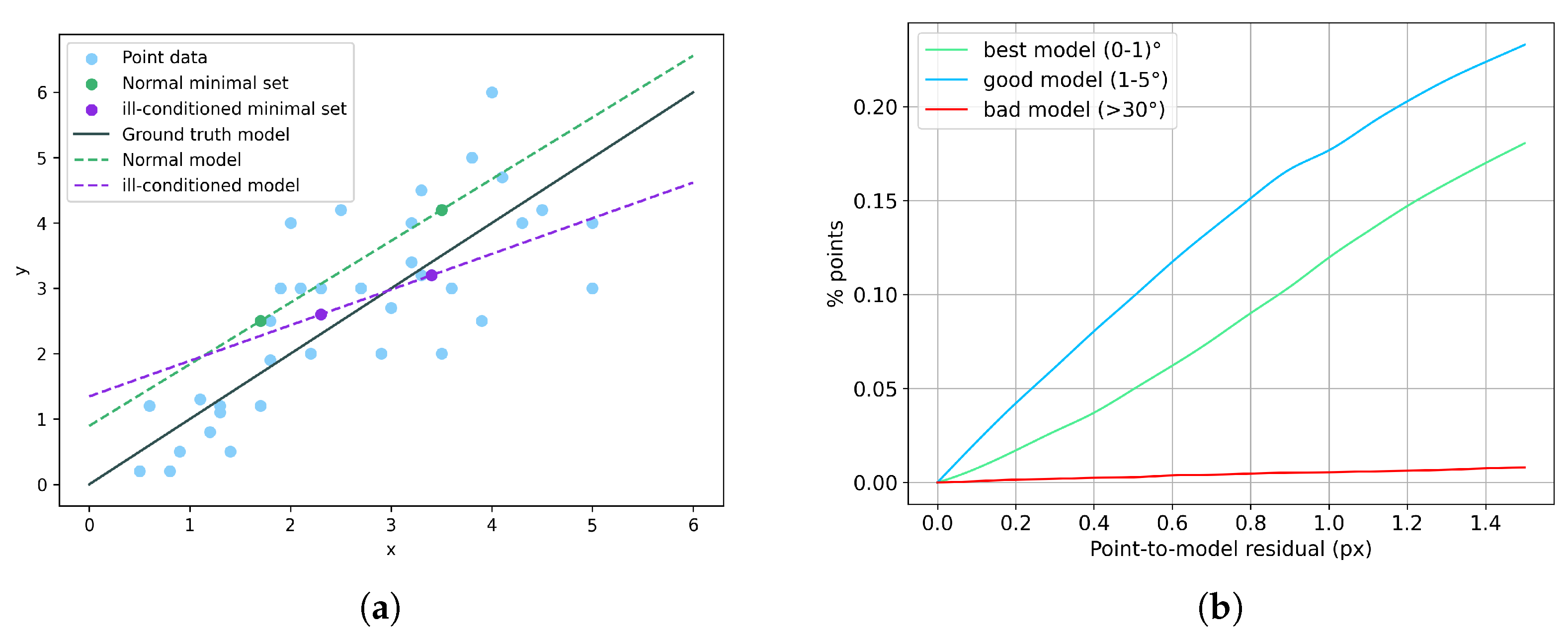
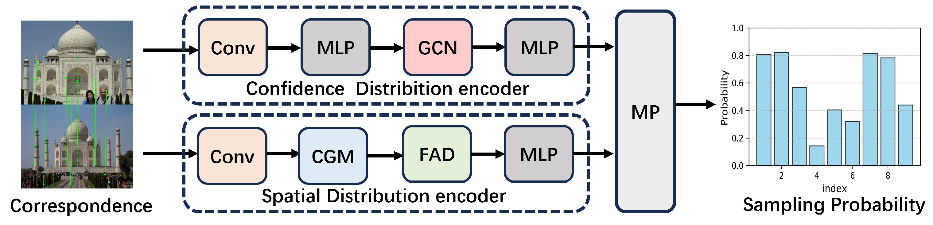
• We reveal the suboptimality in robust estimation models that rely solely on confidence for evaluation. To address this, we propose SA-Net, a dual-branch network that integrates spatial distribution information, mitigating over-reliance on confidence to improve optimization.
• To improve the model’s spatial perception, we introduce the Cluster-based Mapping and FPS Aggregate Dispatch block, which explore feature point relationships from both global and local perspectives. Additionally, we utilize Chamfer Loss to constrain the sampling distribution.
• Compared with state-of-the-art methods, SA-Net achieves superior results in real-world scenarios on fundamental and essential matrix estimation.

2. Related Works

Since the RANSAC [11] method was proposed, many methods based on RANSAC have been developed to enhance the effectiveness of the RANSAC method. The RANSAC method is an algorithm to find the best model and inliers conforming to a model from a set of data. It first randomly selects a certain subset of data from the set to construct a model. After obtaining the model, its quality is determined by a predefined threshold. Once the RANSAC model is obtained, it selects which data points in the set are inliers and which are outliers. RANSAC iterates this process continuously until it reaches the set maximum number of iterations. In the process mentioned above, many methods have made improvements to the RANSAC pipeline as shown in Figure 4 and achieved better results than RANSAC [8,9,10,12,13,14,15,16,17,18,19,20,21].

When sampling correspondence in RANSAC, all point pairs contribute equally to the model evaluation. However, we can roughly assess the correctness of the matches by considering factors such as the confidence of the matches and other relevant information. N adjacent points sample consensus (NAPSAC) [14] considers that inliers should be concentrated around a hyperplane, while outliers are uniformly distributed outside a spherical region. It performs point sampling by adjusting the radius of the hypersphere. Locally optimized random sample consensus (LO-RANSAC) [12] uses local optimization to reweight all inliers to avoid the influence of outliers. During each sampling, points are selected from the inliers. Progressive sample consensus (PROSAC) [22] uses a probabilistic prior to guide the sampling process, where points with higher confidence are more likely to be considered, thus accelerating the computation process. Group sample consensus (GroupSAC) [15] introduces the concept of grouping on top of NAPSAC, grouping points based on their similarity. Points within the same group are more likely to be inliers if they exhibit strong intra-group consistency. Universal sample consensus (USAC) [16] summarizes the advantages of previous work and forms a standard framework. In [18], graph-cut random sample consensus ((GC-RANSAC) abstracts points into a graph, assuming that neighboring points have the same inlier/outlier classification to optimize the model. MAGSAC [8] and MAGSAC++ [9] avoid manually setting thresholds and evaluate the model by marginalizing thresholds and using point scores as weights. Rydell et al. [23] revisited the Sampson approximation in epipolar geometry and explained when the Sampson distance approximation works most effectively.

Currently, some methods have also integrated deep learning into the pipeline of RANSAC and achieved promising results by combining traditional model quality evaluation steps. Differentiable random sample consensus (DSAC) [17] designs neural networks to predict sampling distributions and model scores separately. Neural-guided random sample consensus (NG-RANSAC) [19] uses the distance from the points to the ground truth model as supervision signals, which achieves probabilistic sampling for points. However, in the above works, the sampling process remained non-differentiable. The emergence of Gumbel-Softmax [24] bridged the gap in the sampling process, where generalized differentiable random sample consensus (D-RANSAC) firstly applies Gumbel-Softmax [24] to the RANSAC pipeline, making the entire RANSAC process end to end. Recently, there have also been some methods that apply other deep learning paradigms, such as [21,25]. Reinforcement learning sample consensus (RLSAC) [25] firstly applies reinforcement learning paradigms to robust estimation. Bayesian network random consensus (BANSAC) [21] utilizes Bayesian networks to update the probability of individual points, continuously iterating and optimizing the model. Ding et al. [26] proposed a depth-based method to estimate the fundamental matrix through the relative depths between corresponding points. Fan et al. [27] started from anchored objects, leveraging the power of the pre-trained large-scale 2D foundation model, and adopted a framework with hierarchical feature representation and 3D geometry principles to estimate the relative camera pose between object prompts and the target object in new views. At the same time, ref. [28] proposed a random epipolar constraint loss function and a lightweight optical flow estimation framework to constrain the neural network and enhance the model’s generalization ability. Parallel sample consensus (PARSAC) [29] predicts multiple sets of sample and inlier weights to determine the model parameters for each potential instance in parallel. Neurally filtered sample consensus (NeFSAC) [10] firstly introduced the concept of poor conditioning. NeFSAC holds that even if each point in the minimal point set has particularly small errors, certain combinations can still lead to significant errors in model estimation due to the inconsistent spatial relationships among some points, thus preventing the estimation of models using bad minimal samples.

Our work follow the concept of NeFSAC and introduces a novel end-to-end neural network. Instead of solely relying on datasets to constrain the neural network training process, we incorporate a specific positional-aware module called spatial encoder to address this problem.

3. Methods

SA-Net processes both geometric and auxiliary information from matches to generate a sampling distribution that guides model computation. As illustrated in Figure 5, the network consists of two main components: the spatial distribution encoder and the confidence distribution encoder. Each encoder plays a critical role in refining the sampling process, and their functionalities are detailed in the following sections.

3.1. Confidence Distribution Encoder

We aim to map match information, represented by $X_c\in {\mathbb{R}}^{N\times 7}$, to a probability distribution within $[0,1]$, the details as shown in Figure 6. Here, $X_c$ includes both geometric and additional information, with 7 channels representing position and other details. Then, the match information $X_c$ is processed by the confidence distribution encoder. Initially, a series of ResNet blocks [30] with shared weights transforms $X_c$ to a higher-dimensional space. Subsequently, the group layer from CLNet [31] aggregates the local consensus features. A 1 × 1 MLP kernel is used to derive the probability distribution $p_l$ of these aggregated features. The adjacency matrix is constructed by multiplying $p_l$ with ${p_l}^T$. Enhanced local features are then input into a Graph Convolution Network (GCN) [32] to integrate the global match features, with this process iterated to strengthen the global features and reduce incorrect matches. Finally, a 1 × 1 MLP kernel is applied to produce the confidence probability distribution $p_{con}$.

3.2. Spatial Probability Distribution Encoder

The purpose of the spatial distribution encoder is to extract meaningful geometric relationships from the input data, which is essential for capturing spatial correlations between matches as in Figure 7. And the detail is shown in Figure 8. The input data, represented as ${\mathbf{X}}_s={\left\{{\mathrm{x}}_i^s\right\}}_{i=1}^N\in {\mathbb{R}}^{N\times 4}$, contain geometric information for image matching. To effectively capture this information, ResNet blocks are applied to project ${\mathrm{x}}_i^s$ into a higher-dimensional feature space, generating the feature map $F_s={\left\{f_i^s\right\}}_{i=1}^N$. This transformation enhances the model’s ability to learn spatial relationships, providing a richer feature representation for subsequent encoding processes.

Cluster-based Graph Mapping Block. The Cluster-based Graph Mapping block is proposed to group similar features into clusters and propagate information within clusters. This helps model the spatial relationships more effectively by aggregating information across nodes. To achieve this, we treat each feature $f_s^i$ as a node and divide the nodes into $k_c$ clusters. A sparse graph network is then constructed to facilitate communication between nodes within clusters. The clustering matrix $M={\left\{m_{ij}\right\}}_{i,j=1}^N$ is used to mapping intra-cluster relationships, where $m_{ij}=1$ if nodes i and j belong to the same cluster:

$$m_{ij}=\left\{\begin{array}{c}1,c_i=c_j\hfill \\ 0,\mathrm{otherwise}\hfill \end{array}\right.$$

(1)

Then, to obtain the cluster feature $F_{clu}$, the process of interaction can be expressed as

$$\begin{array}{c}(Q_s,K_s,V_s)=Linea{r}_{(Q,K,V)}\left(F_s\right)\hfill \\ F_{clu}=At{t}_{clu}\left(F_s\right)=M·softMax\left({\displaystyle \frac{Q_s{K}_s^T}{\sqrt{dim}}}\right)V_s,\hfill \end{array}$$

(2)

where Q, K, and V represent the query, key, and value vectors corresponding to the respective features.

FPS Aggregation Dispatch Block. This block selects representative points (anchors) from geometric data to effectively propagate global spatial information to the local context. The process starts with the random selection of an initial data match from $X_s$, forming the starting point for the anchor set $X_{fps}$. We then compute the distance between each remaining point and the current anchor set, iteratively adding the farthest point until $X_{fps}$ contains $k_s$ points.

After obtaining the anchor set, FPS Attention extracts the corresponding features from the feature map, and these anchor features are aggregated using a self-attention mechanism, which captures key global spatial relationships.

To disseminate this global information into the local context, KNN Attention is applied. The aggregated anchor features are adaptively distributed to surrounding points based on their feature similarity, facilitating interaction and feature sharing within the local region. A group of $k_n$ points is selected around each anchor to form local clusters, where the anchor feature is denoted as $f_{an}$ and the local context features as $f_{loc}$. The dispatched local context features $f_{loc}^{\prime }$ are computed as follows.

$$\begin{array}{c}(Q_d,K_d,V_d)=Linea{r}_{(Q,K,V)}(f_{an},f_{loc},f_{loc})\hfill \\ f_{loc}^{\prime }=softMax\left({\displaystyle \frac{Q_d{K}_d^T}{\sqrt{dim}}}\right)V_d,\hfill \end{array}$$

(3)

and sampling preference $p_{spa}\in {\mathbb{R}}^{B\times L\times N}$ is obtained for the data point set by passing $F_{fps}$ through several 1 × 1 MLP layers.

Multi-Perspective Block. Since both clustering and sampling operations involve randomness, a single poor sampling or clustering result may lead to suboptimal results. To promote diversity in sampling, the spatial encoder is executed in parallel with L heads. Additionally, the confidence distribution probabilities are combined with the sampling preference probabilities. A hyperparameter $\delta$ is introduced to balance the two weights and derive the final sampling probability $p=p_{con}+\delta p_{spa}$.

3.3. Loss Function

In RANSAC and its variant methods, a predetermined threshold is used to classify data points. Data points in the set with a distance to the model less than the threshold are considered inliers, while those with a greater distance are considered outliers. Some methods follow the RANSAC approach to design their loss functions. For example, ref. [17] applies soft probabilistic hypothesis selection to optimize the model. Other algorithms [31] apply cross-entropy loss to model optimization based on the idea of match exclusion. They also use geometry-induced losses [19] to link the estimated model quality with the distribution of inliers.

Inspired and influenced by these works, we compare our estimated model with the ground truth model to constrain the model’s convergence. We use SVD decomposition [33] to turn the solution $\widehat{\theta }$ into rotation and translation $(\widehat{R},\widehat{t})$. We know that the rotation error ${\epsilon }_{\mathbf{R}}$ and translation error ${\epsilon }_{\mathbf{t}}$ can be calculated using the following formulas:

$$\begin{array}{c}{\epsilon }_R(\widehat{R},R)={cos}^{-1}\left(\left(\mathrm{tr}\left(\widehat{R}{R}^{\mathrm{T}}\right)-1\right)/2\right)\hfill \\ {\epsilon }_t(\widehat{t},t)={cos}^{-1}\left({\displaystyle \frac{{\widehat{t}}^{\mathrm{T}}t}{\left|\right|\widehat{t}\left|\right|·\left|\right|t\left|\right|}}\right)\hfill \end{array}$$

(4)

where R and t are the ground truth rotation matrix and ground truth translation matrix, respectively. The pose loss is subsequently defined as follows:

$$L_{pose}={\displaystyle \frac{1}{2}}({\epsilon }_R(\widehat{R},R)+{\epsilon }_t(\widehat{t},t)),$$

(5)

The average symmetric epipolar error is defined as follows:

$$L_{epi}={\displaystyle \frac{1}{\left|\mathcal{I}\right|}}\sum _{i\in \mathcal{I}}{\epsilon }_{epi}\left(\theta ,{\Phi }_i\right),$$

(6)

where $\mathcal{I}$ is the set of inliers selected based on the ground truth model, and $\theta$ is the ground truth model. ${\Phi }_i$ is the positional information of data item i, and ${\epsilon }_{epi}$ is the residual error corresponding to the data item.

Chamfer Loss $L_{cham}$ is applied to constrain the spatial distribution of the sampling to be relatively sparse:

$$L_{cham}(X_s,X_m)={\displaystyle \frac{1}{|X_s|}}\sum _{{\mathrm{x}}_s\in X_s}\underset{{\mathrm{x}}_m\in X_m}{min}\left|\right|{\mathrm{x}}_s-{\mathrm{x}}_m{\left|\right|}_2^2$$

(7)

Here, $X_m$ represents the matches in the minimal sampling set. The ultimate optimization objective is defined as

$$L=L_{pose}+\alpha L_{epi}+\beta L_{cham}$$

(8)

4. Experiments

The proposed SA-Net is trained on an Nvidia RTX A6000 GPU (Nvidia, Santa Clara, CA, USA) for 15 epochs, with a batch size of 64 and a learning rate of ${10}^{-5}$. The number of clusters in the CGM block and the anchor parameter $k_s$ are both set to 64, while the KNN parameter $k_n$ is set to 32. To increase sampling diversity, we configure the number of parallel layers L in the spatial distribution encoder as 4 and assign the weight of probabilistic bargaining mechanism to 0.1. For the loss function, the parameters $\alpha$ and $\beta$ are both set to 0.1. We train the model using pre-detected RootSIFT features [34] from the PhotoTourism dataset [35], which contains on 4950 image pairs from the St. Peter’s Square scene, split into training and validation sets at a 3:1 ratio. The remaining 12 scenes are used exclusively for testing. For model selection, we follow the MAGSAC++ [9] for model evaluation.

4.1. Fundamental Matrix Estimation

We follow D-RANSAC [20] and use the eight-point algorithm on four preferences sampling distributions. As shown in

Table 1. The F1 scores (each, average in last row) for F matrix estimation on 6K image pairs from the PhotoTourism dataset [35]. Best results are in bold, and the second best are underlined.

Scene/Method	RANSAC	MAGSAC++	OANet	CLNet	NG-RANSAC	RLSAC	D-RANSAC	SA-Net
Taj Mahal	42.21	58.63	54.13	56.22	57.65	54.98	59.66	60.51
Sacre Coeur	45.83	52.11	47.28	48.10	51.03	53.71	53.09	55.08
Trevi Fountain	31.77	35.93	29.32	30.07	36.25	34.89	35.97	39.45
Pantheon Exterior	58.20	63.44	51.39	55.79	59.81	61.49	65.38	66.97
Brandenburg Gate	36.95	39.32	37.03	38.48	39.20	41.94	41.43	44.91
Colosseum Exterior	46.80	51.34	43.58	47.87	53.21	56.86	55.43	56.08
Buckingham Palace	25.65	29.76	25.93	27.81	29.88	29.13	30.71	33.79
Grand Place Brussels	29.75	33.84	29.56	33.52	35.39	34.35	35.56	37.52
Palace of Westminster	31.73	33.85	31.65	32.72	35.12	34.27	34.92	39.88
Prague Old Town Square	35.56	38.73	34.32	37.34	39.43	38.31	39.72	41.23
Notre-Dame Front Facade	37.93	39.84	34.58	36.85	39.74	39.47	43.51	45.63
Westminster Abbey	52.06	52.89	43.38	49.03	51.27	50.41	52.04	52.57
Avg	39.54	44.14	38.51	41.15	44.00	44.15	45.61	47.80

, SA-Net outperforms existing traditional and deep learning methods in most scenes, and the average F1 score of our method surpasses the second-best method by 2.19 points. In some challenging scenes, such as Buckingham Palace and the Palace of Westminster, our method significantly improves accuracy compared to other methods. Furthermore, we show the cumulative distribution functions (CDFs) of epipolar errors. The epipolar errors are calculated from the 6K test image pairs in PhotoTourism. As Figure 9 shown, the curve of our method is the highest in the figure, and our advantage over other methods is more pronounced at lower epipolar errors. This demonstrates that our method excels at selecting the relatively more accurate model from a set of high-precision models.

4.2. Essential Matrix Estimation

In essential matrix estimation, we decompose E into its rotation and translation matrix, and subsequently calculate their respective errors. The area under the curve (AUC) is then computed with thresholds at 5°, 10°, and 20°. As presented in

Table 2. The average AUC scores and run-time of SA-Net and comparison methods over 12 scenes on RootSIFT [34] matches. Best results are in bold, and the second best are underlined.

Method	AUC@5°	AUC@10°	AUC@20°	Run-Time (ms)
LMEDS	0.237	0.292	0.345	21
RANSAC	0.251	0.334	0.394	42
GC-RANSAC	0.315	0.375	0.413	81
MAGSAC	0.355	0.405	0.457	102
MAGSAC++	0.354	0.411	0.459	68
OANet	0.259	0.323	0.374	25
CLNet	0.334	0.395	0.449	31
NG-RANSAC	0.369	0.413	0.464	52
D-RANSAC	0.394	0.426	0.501	61
SA-Net	0.436	0.442	0.524	78

, RootSIFT features and the SNN ratio [36] are utilized to derive matching information and confidence, which serve as inputs to the model for estimating the essential matrix. Our approach outperforms both traditional and deep learning-based methods, achieving the highest accuracy. However, we fall behind some methods in terms of inference time.

4.3. Ablation Study

To analyze the effects of each component in SA-Net, we perform detailed ablation studies on the PhotoTourism dataset. We divide our network into the following components: confidence distribution encoder (CDE), Cluster-based Graph Mapping block (CGM), FPS Aggregation Dispatch Block (FAD) and Chamfer Loss (CL). We ablate the structures within our network to demonstrate the importance of each component. The result of the ablation study is shown in

Table 3. Ablation study of SA-Net on essential matrix estimation using PhotoTourism dataset. Best results are in bold, and the second best are underlined.

CDE	CGM	FAD	CL	AUC
				@5°	@10°	@20°
✔				0.378	0.421	0.483
✔	✔			0.412	0.428	0.513
✔		✔	✔	0.401	0.434	0.517
✔	✔	✔	✔	0.436	0.442	0.524

. We conduct our tests on 6000 images from PhotoTourism, maintaining the same experimental setup and parameters as in Table 1. A neural network with only the Con. module is used as the baseline method to verify the improvement in accuracy brought by the other network modules. Based on the baseline, we retrain four groups of networks: CDE, CDE+CGM, CDE+FAD+CL, and the full version of the network. The CDE+CGM combination improves by 0.03 at @5° compared to the baseline, while the CDE+FAD+CL combination shows more significant improvements at @10° and @20°. The full network achieves the best performance across all metrics.

Meanwhile, we posit that increasing the number of sampling preferences does not inherently yield better results. To test this hypothesis, we conduct ablation experiments with varying values of L, reporting the F1 scores, epipolar error, and inference time (see

Table 4. The effect of fixing or varying the number of parallel layers L in the spatial distribution encoder. We report the F1 score, mean epipolar error, and run-time on the fundamental matrix estimation from PhotoTourism [35]. Best results are in bold, and the second best are underlined.

Settings/Metric	F1 Score (%)	Med. Epi. Error (px)	Run-Time (ms)
$L=1$	44.29	2.61	21
$L=2$	47.50	1.83	25
$L=4$	49.31	1.07	34
$L=8$	43.77	4.12	46
$L=16$	34.81	13.23	73

). Our findings indicate that when the number of sampling preferences is too small, the model is prone to becoming trapped in local optima. Conversely, when the number of preferences is too large, the sampling per preference becomes insufficient, resulting in a notable decline in overall accuracy.

4.4. Visualization

To understand the impact of our spatial encoder on the confidence distribution of match sampling, we conduct visualization experiments. We explore the confidence distribution of matches in different spatial regions as shown in Figure 10. We select the Brandenburg Gate, Buckingham Palace, and the Taj Mahal for our visualization experiments. We find that, in RANSAC and NG-RANSAC, the lack of constraints on the spatial distance of matches can lead to sampling pairs with similar spatial distances, which degrades the results of the relative pose estimation. SA-Net sampling maintains a relatively sparse distribution in space and achieves better results in relative pose estimation.

5. Discussion

In traditional robust model estimation algorithms, each point is treated with equal importance. This approach often results in noisy points being included in the model estimation, thereby reducing its accuracy. In deep learning-based methods, many researchers typically use the distance from data points to the model (epipolar distance in our paper) as the direct optimization objective. However, through experiments, we observe that the epipolar distance is not the sole factor affecting model accuracy. To address the shortcomings of the two methods, we propose a dual-branch neural network that simultaneously focuses on both the confidence information and spatial location information of the data points. Experiments show that our approach achieves optimal performance in most scenarios. Additionally, we conduct ablation experiments to evaluate the performance improvement contributed by each module. We find that all of our modules complement each other, with the MP module effectively solving the randomness issue caused by farthest point sampling and clustering operations. Furthermore, we experiment with the number of layers in the MP module and find that $L=4$ is optimal. Too many layers may lead to insufficient sampling at each layer, while too few layers may expose the model to random interference, affecting the experimental results. Although our work achieves relatively good performance, in order to avoid the spatial randomness introduced by farthest point sampling and clustering operations, we introduce a multi-layer parallel neural network to eliminate this randomness. This, however, significantly increases the number of parameters in the network and sacrifices efficiency in terms of the training and inference time.

6. Conclusions

In this paper, a dual-branch network SA-Net is proposed to incorporate spatial distribution encoder and confidence distribution encoder. SA-Net leverages the accuracy of matching data and the spatial distribution of minimal sets. In the spatial distribution encoder, the Cluster-based Graph Mapping block enhances the correlation between domain data through clustering, while the FPS Aggregation Dispatch Block employs an aggregate dispatch strategy to progressively propagate global information to local neighborhoods. Given the inherent randomness of both clustering and FPS, we parallelize multiple spatial distribution encoder layers to introduce diversity in the spatial distribution of the samples, thereby avoiding suboptimal results. Meanwhile, Chamfer Loss is introduced to constrain the spatial distribution of the sampling. Experimental results demonstrate that our approach outperforms current traditional and deep learning methods. However, in order to avoid randomness, our method introduces a multi-layer parallel neural network, which results in the algorithm not achieving optimal efficiency. In the future, we will focus on balancing the algorithm’s performance and efficiency, aiming to achieve relatively better results while also making the algorithm more lightweight.

References

1. Torr, P.H.; Murray, D.W. Outlier detection and motion segmentation. In Proceedings of the Sensor Fusion VI. SPIE, Boston, MA, USA, 7–10 September 1993; Volume 2059, pp. 432–443. [Google Scholar]
2. Schönberger, J.L.; Zheng, E.; Frahm, J.M.; Pollefeys, M. Pixelwise view selection for unstructured multi-view stereo. In Proceedings of the Computer Vision–ECCV 2016: 14th European Conference, Amsterdam, The Netherlands, 11–14 October 201; Proceedings, Part III 14. pp. 501–518.
3. Ding, L.; Sharma, G. Fusing structure from motion and lidar for dense accurate depth map estimation. In Proceedings of the 2017 IEEE International Conference on Acoustics, Speech and Signal Processing (ICASSP), New Orleans, LA, USA, 5–9 March 2017; pp. 1283–1287. [Google Scholar]
4. Schonberger, J.L.; Frahm, J.M. Structure-from-motion revisited. In Proceedings of the IEEE Conference on Computer Vision and Pattern Recognition, Las Vegas, NV, USA, 27–30 June 2016; pp. 4104–4113. [Google Scholar]
5. Capel, D. Image mosaicing. In Image Mosaicing and Super-Resolution; Springer: Berlin/Heidelberg, Germany, 2004; pp. 47–79. [Google Scholar]
6. Chen, Z.; Liu, T.; Huang, J.J.; Zhao, W.; Bi, X.; Wang, M. Invertible Mosaic Image Hiding Network for Very Large Capacity Image Steganography. In Proceedings of the ICASSP 2024–2024 IEEE International Conference on Acoustics, Speech and Signal Processing (ICASSP), Seoul, Republic of Korea, 14–19 April 2024; pp. 4520–4524. [Google Scholar]
7. Mei, X.; Ramachandran, M.; Zhou, S.K. Video background retrieval using mosaic images. In Proceedings of the ICASSP 2005–2005 IEEE International Conference on Acoustics, Speech and Signal Processing (ICASSP), Philadelphia, PA, USA, 18–23 March 2005; Volume 2, pp. ii-441–ii-444. [Google Scholar]
8. Barath, D.; Matas, J.; Noskova, J. MAGSAC: Marginalizing sample consensus. In Proceedings of the IEEE/CVF Conference on Computer Vision and Pattern Recognition, Long Beach, CA, USA, 15–20 June 2019; pp. 10197–10205. [Google Scholar]
9. Barath, D.; Noskova, J.; Ivashechkin, M.; Matas, J. MAGSAC++, a fast, reliable and accurate robust estimator. In Proceedings of the IEEE/CVF Conference on Computer Vision and Pattern Recognition, Seattle, WC, USA, 14–19 June 2020; pp. 1304–1312. [Google Scholar]
10. Cavalli, L.; Pollefeys, M.; Barath, D. NeFSAC: Neurally filtered minimal samples. In Proceedings of the European Conference on Computer Vision, Tel Aviv, Israel, 23–27 October 2022; pp. 351–366. [Google Scholar]
11. Fischler, M.A.; Bolles, R.C. Random sample consensus: A paradigm for model fitting with applications to image analysis and automated cartography. Commun. ACM 1981, 24, 381–395. [Google Scholar] [CrossRef]
12. Chum, O.; Matas, J.; Kittler, J. Locally optimized RANSAC. In Proceedings of the Pattern Recognition: 25th DAGM Symposium, Magdeburg, Germany, 10–12 September 2003; Proceedings 25. pp. 236–243. [Google Scholar]
13. Torr, P.H.; Zisserman, A. MLESAC: A new robust estimator with application to estimating image geometry. Comput. Vis. Image Underst. 2000, 78, 138–156. [Google Scholar] [CrossRef]
14. Torr, P.H.; Nasuto, S.J.; Bishop, J.M. Napsac: High noise, high dimensional robust estimation-it’s in the bag. In Proceedings of the British Machine Vision Conference (BMVC), Cardiff, UK, 2–5 September 2002; Volume 2, p. 3. [Google Scholar]
15. Ni, K.; Jin, H.; Dellaert, F. GroupSAC: Efficient consensus in the presence of groupings. In Proceedings of the 2009 IEEE 12th International Conference on Computer Vision, Kyoto, Japan, 29 September–2 October 2009; pp. 2193–2200. [Google Scholar]
16. Raguram, R.; Chum, O.; Pollefeys, M.; Matas, J.; Frahm, J.M. USAC: A universal framework for random sample consensus. IEEE Trans. Pattern Anal. Mach. Intell. 2012, 35, 2022–2038. [Google Scholar] [CrossRef] [PubMed]
17. Brachmann, E.; Krull, A.; Nowozin, S.; Shotton, J.; Michel, F.; Gumhold, S.; Rother, C. Dsac-differentiable ransac for camera localization. In Proceedings of the IEEE Conference on Computer Vision and Pattern Recognition, Honolulu, HI, USA, 21–26 July 2017; pp. 6684–6692. [Google Scholar]
18. Barath, D.; Matas, J. Graph-cut RANSAC. In Proceedings of the IEEE Conference on Computer Vision and Pattern Recognition, Salt Lake City, UT, USA, 18–22 June 2018; pp. 6733–6741. [Google Scholar]
19. Brachmann, E.; Rother, C. Neural-guided RANSAC: Learning where to sample model hypotheses. In Proceedings of the IEEE/CVF International Conference on Computer Vision, Seoul, Republic of Korea, 27 October–2 November 2019; pp. 4322–4331. [Google Scholar]
20. Wei, T.; Patel, Y.; Shekhovtsov, A.; Matas, J.; Barath, D. Generalized differentiable RANSAC. In Proceedings of the IEEE/CVF International Conference on Computer Vision, Paris, France, 1–6 October 2023; pp. 17649–17660. [Google Scholar]
21. Piedade, V.; Miraldo, P. BANSAC: A dynamic BAyesian Network for adaptive SAmple Consensus. In Proceedings of the IEEE/CVF International Conference on Computer Vision, Paris, France, 1–6 October 2023; pp. 3738–3747. [Google Scholar]
22. Chum, O.; Matas, J. Matching with PROSAC-progressive sample consensus. In Proceedings of the 2005 IEEE Computer Society Conference on Computer Vision and Pattern Recognition (CVPR’05), San Diego, CA, USA, 20–26 June 2005; Volume 1, pp. 220–226. [Google Scholar]
23. Rydell, F.; Torres, A.; Larsson, V. Revisiting sampson approximations for geometric estimation problems. In Proceedings of the IEEE/CVF Conference on Computer Vision and Pattern Recognition, Seattle, WA, USA, 16–22 June 2024; pp. 4990–4998. [Google Scholar]
24. Jang, E.; Gu, S.; Poole, B. Categorical reparameterization with gumbel-softmax. arXiv 2016, arXiv:1611.01144. [Google Scholar]
25. Nie, C.; Wang, G.; Liu, Z.; Cavalli, L.; Pollefeys, M.; Wang, H. RLSAC: Reinforcement Learning enhanced Sample Consensus for End-to-End Robust Estimation. In Proceedings of the IEEE/CVF International Conference on Computer Vision, Paris, France, 1–6 October 2023; pp. 9891–9900. [Google Scholar]
26. Ding, Y.; Vávra, V.; Bhayani, S.; Wu, Q.; Yang, J.; Kukelova, Z. Fundamental matrix estimation using relative depths. In Proceedings of the European Conference on Computer Vision, Milan, Italy, 29 September–4 October 2024; Springer: Berlin/Heidelberg, Germany, 2025; pp. 142–159. [Google Scholar]
27. Fan, Z.; Pan, P.; Wang, P.; Jiang, Y.; Xu, D.; Wang, Z. POPE: 6-DoF Promptable Pose Estimation of Any Object in Any Scene with One Reference. In Proceedings of the IEEE/CVF Conference on Computer Vision and Pattern Recognition, Seattle, WA, USA, 16–22 June 2024; pp. 7771–7781. [Google Scholar]
28. Fan, Z.; Cai, Z. Random epipolar constraint loss functions for supervised optical flow estimation. Pattern Recognit. 2024, 148, 110141. [Google Scholar] [CrossRef]
29. Kluger, F.; Rosenhahn, B. PARSAC: Accelerating Robust Multi-Model Fitting with Parallel Sample Consensus. In Proceedings of the AAAI Conference on Artificial Intelligence, Vancouver, BC, USA, 20–27 February 2024; Volume 38, pp. 2804–2812. [Google Scholar]
30. He, K.; Zhang, X.; Ren, S.; Sun, J. Deep residual learning for image recognition. In Proceedings of the IEEE Conference on Computer Vision and Pattern Recognition, Las Vegas, NV, USA, 27–30 June 2016; pp. 770–778. [Google Scholar]
31. Zhao, C.; Ge, Y.; Zhu, F.; Zhao, R.; Li, H.; Salzmann, M. Progressive correspondence pruning by consensus learning. In Proceedings of the IEEE/CVF International Conference on Computer Vision, Montreal, QC, Canada, 11–17 October 2021; pp. 6464–6473. [Google Scholar]
32. Kipf, T.N.; Welling, M. Semi-supervised classification with graph convolutional networks. arXiv 2016, arXiv:1609.02907. [Google Scholar]
33. Hartley, R.; Zisserman, A. Multiple View Geometry in Computer Vision; Cambridge University Press: Cambridge, UK, 2003. [Google Scholar]
34. Arandjelović, R.; Zisserman, A. Three things everyone should know to improve object retrieval. In Proceedings of the 2012 IEEE Conference on Computer Vision and Pattern Recognition, Providence, RI, USA, 16–21 June 2012; pp. 2911–2918. [Google Scholar]
35. Jin, Y.; Mishkin, D.; Mishchuk, A.; Matas, J.; Fua, P.; Yi, K.M.; Trulls, E. Image Matching across Wide Baselines: From Paper to Practice. Int. J. Comput. Vis. 2020, 129, 517–547. [Google Scholar] [CrossRef]
36. Lowe, D.G. Object recognition from local scale-invariant features. In Proceedings of the Seventh IEEE International Conference on Computer Vision, Kerkyra, Greece, 20–27 September 1999; Volume 2, pp. 1150–1157. [Google Scholar]
Figure 1. Line fitting example and model residual analysis. (a) Taking 2D line fitting as an example, the solid black line in the figure represents the ground truth model. Although the points in the ill–conditioned minimal set are closer to the ground truth, the fitted line exhibits greater error compared to the one derived from the normal minimal set. (b) Residual analysis of models with varying levels of quality. We analyzed the residual distribution of data for the 1 k minimum sample set selected by models of varying quality. It was observed that the best-performing model did not exhibit the most ideal residual distribution.
Algorithms 18 00065 g001
Figure 2. Visualization of ill–conditioned problems. The red line represents outliers, while the green line represents inliers. When outliers are present, the estimated model exhibits large errors. When all points in the minimal set are inliers but are densely distributed, it can lead to model degradation, which we refer to as the ill-conditioned minimum set. On the other hand, when the points in the minimum set are sparsely distributed and all inliers, the estimated model achieves higher precision.
Algorithms 18 00065 g002
Figure 3. Spatial distribution analysis of good models and best models. We analyze the minimal sets of good models and the best model by calculating the Euclidean distance between the closest points within each minimal set. It is observed that the minimum Euclidean distance in the best model’s minimal set is significantly greater than that in the good models’ minimal sets.
Algorithms 18 00065 g003
Figure 4. Illustration of the robust model estimation process. Both traditional methods and deep learning-based approaches broadly rely on the RANSAC framework. The entire process can be divided into four stages: sampling, model computation, evaluation, and selecting the best model.
Algorithms 18 00065 g004
Figure 5. The architecture of SA-Net. The proposed model consists of the confidence distribution encoder and spatial distribution encoder. The confidence distribution encoder reduces outlier impact by refining confidence scores through group layers and graph neural networks. In the spatial distribution encoder, the Cluster-based Graph Mapping block (CGM) connects clusters, while the sparse graph aggregates spatial information from neighboring areas. Additionally, the FPS Aggregate Dispatch Block (FAD) selects anchor points, allowing global spatial data to influence the local context. The Multi-Perspective Block integrates confidence probabilities and spatial distribution probabilities to derive the final sampling distribution.
Algorithms 18 00065 g005
Figure 6. The architecture of the confidence distribution encoder.The confidence distribution encoder takes the spatial positions of matches and additional information as input. The Res-block maps low-dimensional information to higher dimensions, while the Group Layer aggregates features to explore the consistency among high-dimensional features. The GCN establishes connections between features, effectively eliminating incorrect matches. Finally, the MLP layer reduces the feature dimensions into confidence probability information.
Algorithms 18 00065 g006
Figure 7. The architecture of spatial distribution encoder. The confidence distribution encoder takes the spatial positions of matches as input. Cluster-based graph mapping enables the more effective aggregation of spatial position information within the matching space. The FPS aggregation dispatch mechanism facilitates the efficient transmission of local information to the global context through aggregation and dispatch processes, while also accelerating computation.
Algorithms 18 00065 g007
Figure 8. The detail of spatial distribution encoder and Multi-Perspective Block. The KNN-Attention module is responsible for extracting domain-specific information, while the FPS-Attention module distributes this information through anchor nodes. Due to the inherent randomness of clustering and farthest point sampling, the Multi-Perspective Block effectively integrates multi-layer spatial distributions with single-layer confidence distributions. This fusion mitigates the impact of randomness on model performance.
Algorithms 18 00065 g008
Figure 9. The comparison of RANSAC, GC-RANSAC, MAGSAC, MAGSAC++, OANet, CLNet, NG-RANSAC, D-RANSAC and ours; we show the cumulative distribution functions of the epipolar errors.
Algorithms 18 00065 g009
Figure 10. Visualization of relative pose estimation. The green line represents the sampled matches. Three different scenarios are chosen to visualize our sampling and relative pose estimation results. Error_R represents the error of the rotation matrix, and Error_t represents the error of the translation vector. From top to bottom: Brandenburg Gate, Buckingham Palace, and Taj Mahal.
Algorithms 18 00065 g010