Abstract
This study investigates the use of three different quadrature schemes, as well as an iterative quadrature methodology, to analyze vibrations in magneto-electro-thermo-elastic nanobeams. Individual MATLAB programs for each method are developed with the goal of minimizing errors in comparison to accurate findings, as well as determining the execution time for each strategy. This study shows that the Discrete Singular-Convolution Differential Quadrature Method with a Regularized Shannon Kernel (DSCDQM-RSK) and specified parameters produces the best accurate and efficient results for this particular situation. A subsequent parametric study is carried out to determine the effect of various factors on the vibrated nanobeam, including boundary conditions, material types, linear and nonlinear elastic foundation properties, nonlocal parameters, length-to-thickness ratios, external electric and magnetic potentials, axial forces, and temperature variations. Important discoveries include insights into the relationship between fundamental frequency, linear elastic foundation features, axial loads, external magnetic fields, temperature fluctuations, and material types. According to this study, these findings could be critical in the development of sophisticated nanostructures made from magneto-electro-thermo-elastic materials for use in a variety of electromechanical applications. This would entail utilizing nanobeams’ unique properties in applications such as sensors, resonators, and transducers for nanoelectronics and biology.
1. Introduction
Magneto-electro-thermo-elastic (METE) composites, comprising piezoelectric and piezomagnetic phases, exhibit remarkable energy conversion capabilities, transforming electric, thermal, elastic, and magnetic energy [1,2]. Their versatility has led to widespread adoption in various fields, including vibration control, actuation, sensing, medical devices, health monitoring systems, and energy harvesting [3,4].
This section analyzes the available literature on the analysis of magneto-electro-elastic systems. Wu et al. [5] investigated the static behavior of 3D, doubly curved, functionally graded magneto-electro-elastic shells under combined mechanical, electrical, and magnetic loads. Huang et al. [6] proposed analytical and semi-analytical solutions for anisotropic, functionally graded magneto-electro-elastic beams under arbitrary stresses, based on sinusoidal series expansions. Chang [7] investigated the vibration characteristics of transversely isotropic magneto-electro-elastic rectangular plates, considering various vibration conditions (free, deterministic, and random) within fluid environments. Ansari et al. [8] developed a nonlocal, geometrically nonlinear beam model for magneto-electro-thermo-elastic nanobeams subjected to external electric voltage, magnetic potential, and temperature changes. Finally, Ke et al. [9] analyzed the free vibration of embedded magneto-electro-elastic cylindrical nanoshells using Love’s shell theory. These studies collectively provide a foundation for understanding the diverse mechanical and vibrational behaviors of magneto-electro-elastic materials across different structural configurations.
Prior research has examined the response of magneto-electro-elastic materials under various loading conditions. Wu et al. [5] investigated the static behavior of three-dimensional (3D), doubly curved, functionally graded magneto-electro-elastic shells subjected to combined mechanical, electrical, and magnetic loads. Huang et al. [6] developed analytical and semi-analytical solutions for anisotropic, functionally graded magneto-electro-elastic beams under arbitrary loading. These studies provide a foundation for understanding the complex interactions between mechanical, electrical, and magnetic fields within these materials. Chang [7] studied the vibration characteristics of transversely isotropic magneto-electro-elastic rectangular plates, considering free, deterministic, and random vibrations in fluid environments. Furthermore, studies have explored the behavior of magneto-electro-elastic nanostructures. Ansari et al. [8] developed a nonlocal, geometrically nonlinear beam model to analyze the behavior of magneto-electro-thermo-elastic nanobeams under various external stimuli. Ke et al. [9] investigated the free vibration properties of embedded magneto-electro-elastic cylindrical nanoshells, considering size-dependent effects.
The field has seen substantial growth, particularly in the investigation of magneto-electro-thermo-elastic (METE) nanomaterials and nanostructures. Studies have focused on materials such as BiFeO3, BiTiO3-CoFe2O4, NiFe2O4-PZT, and various nanowire and nanobeam configurations [10,11]. The recent incorporation of PTZ-5H-COFe2O4 further expands the potential applications of these materials.
The investigation of nanoscale phenomena frequently employs nonlocal elasticity theory [12,13]. While experimental characterization at the nanoscale level presents significant challenges, and molecular dynamics simulations incur high computational costs, continuum models remain crucial for nanostructure research [14,15,16]. However, compelling evidence suggests that the nonlocal effect, arising from the inherent small-length scales, significantly influences the mechanical properties of nanostructures [15,16,17]. This necessitates the incorporation of nonlocal considerations into traditional structural theories to accurately capture the size-dependent behavior observed in these systems [18].
Numerous recent publications have focused on exploring the static and dynamic characteristics of magneto-electro-thermo-Elastic (METE) nanobeams. These works introduce exact and semi-analytical techniques for addressing linear free and forced vibrations, as well as buckling phenomena in nanobeams [19,20,21]. Additionally, alternative numerical approaches such as finite element analysis [22], meshless methods [23], higher-order B-spline finite strip modeling [24], and Rayleigh-Ritz methods [25] have been investigated for tackling these issues. However, all these methodologies demand a significant number of grid points and substantial computational resources to achieve a satisfactory level of precision.
The Polynomial-Based Differential Quadrature Method (PDQM) has been proven to be able to produce correct results with fewer grid points [26,27,28,29,30], in contrast to many numerical methods [31,32,33]. More reliable substitutes are provided by the Discrete Singular-Convolution Differential Quadrature Method (DSCDQM) [34] and the Sinc Differential Quadrature Method (SDQM) [35]. The selection of shape functions, such as the Regularized Shannon Kernel (RSK), Delta Lagrange Kernel (DLK), and cardinal sine function, which enhance solution convergence and stability, is crucial to the efficacy of these techniques [36,37,38,39,40].
Using the Sinc Differential Quadrature Method (SDQM) and Discrete Singular-Convolution Differential Quadrature Method (DSCDQM), this study examines the vibration properties of magneto-electro-thermo-elastic (METE) nanobeams sitting on nonlinear elastic substrates. Although there are several numerical methods [31,32,33], the PDQM has been proven to be able to provide precise results using fewer grid points [26,27,28,29,30]. Better accuracy and stability are provided by the SDQM [35] and DSCDQM [34] than by the conventional Polynomial-Based DQM. To improve the convergence and stability of the numerical solutions, these techniques rely on the selection of suitable shape functions, such as the Regularized Shannon Kernel (RSK), Delta Lagrange Kernel (DLK), and cardinal sine function [36,37,38,39,40]. By creating innovative numerical algorithms and comparing them to proven analytical and numerical results, this study pioneers the application of the SDQM and DSCDQM to this particular situation.
The impact of various parameters on the natural frequencies and mode shapes of the METE nanobeams are analyzed through a thorough parametric investigation. Axial loads, external magnetic potentials, temperature fluctuations, boundary conditions, material qualities, nonlocal parameters, axial loads, nonlinear and linear elastic foundations, and aspect ratios are some of these variables. The structure of this paper is as follows: the mathematical formulation is explained in depth in Section 2, the numerical methods are described in Section 3, the results and discussion are presented in Section 4 and Section 5, and the main conclusions and future research areas are discussed in Section 6.
2. Formulation of the Problem
Consider a METE nanobeam of dimensions subjected to various external stimuli. The beam is exposed to an electric voltage, , a magnetic potential, , a temperature change, , and a mechanical potential, . Moreover, the beam is supported by a nonlinear elastic foundation, which is defined by the stiffness coefficients , , and , representing linear and nonlinear characteristics, respectively, as depicted in Figure 1.
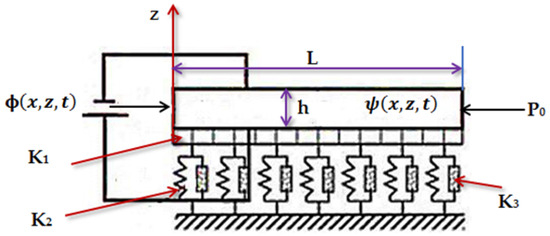
Figure 1.
Schematic of METE nanobeam on nonlinear foundation.
Employing Eringen’s nonlocal elasticity theory, the governing equations for a homogeneous, nonlocal piezoelectric solid in the absence of body forces are presented as follows [9]:
Additionally, the differential form of the integral constitutive relations is as follows [8,9]:
Within this framework, , and ∈ correspond to the electric displacement, electric field, elastic constant, piezoelectric constant, mass density, strain, stress, electric constant, pyroelectric constant, and dielectric constants, respectively. These parameters exhibit variability contingent upon the specific material type. The function characterizes nonlocal attenuation and is embedded into the constitutive formulas at the point of reference . In this context, represents the Euclidean distance. denotes the Laplace operator. , where a is an internal characteristic length and is a nondimensional material constant denoting the scale coefficient that clarifies the size effect on the behavior of structures at the nanoscale. Numerical simulations based on the lattice dynamics [6,19] or experimental techniques can be used to find the value .
The nonlocal constitutive Equations (5) and (6) can be roughly represented as follows, as shown in Figure 1:
where .
The governing equations of motion are obtained using Hamilton’s principle, as outlined in the reference [31].
The boundary conditions are derived by assuming zero electric and magnetic potential at the ends of the nanobeam, as outlined in the reference [35].
In the case of clamped (C) boundary conditions,
In the case of hinged (H) boundary conditions,
where , and denote the transverse displacement, rotation, electric potential, and magnetic potential, respectively. The parameter is a scale coefficient that incorporates the influence of small-scale effects. The shear correction factor k is set to , which is a commonly used value for macroscale beams [31,32,33].
Here, , and denote the normal forces caused by the external electrical potential , the magnetic potential , the temperature variation , and the mechanical potential , respectively. The coefficients , and are associated with thermal, piezoelectric, and piezomagnetic properties, respectively [41].
The current approach, employing Equation (19), represents a simplified treatment of the thermal environment, neglecting the complexities inherent in transient heat transfer processes. Generalized thermoelasticity theories, such as Lord–Shulman (LS) or Green–Lindsay (GL) models, offer a more realistic representation by incorporating time-dependent heat conduction effects and relaxation times. These models account for the finite speed of heat propagation, a phenomenon absent in the classical coupled thermoelasticity theory implicitly used in Equation (19).
The limitations of Equation (19) are significant because it assumes instantaneous thermal equilibrium, which is not accurate at the nanoscale, especially for transient thermal loading. The use of a generalized thermoelasticity theory would lead to a more accurate representation of the temperature field and its influence on the nanobeam’s vibrations. This would involve modifying the governing Equations (11)–(14) to include the appropriate energy equation from the chosen generalized thermoelasticity model (LS or GL). The resulting system of equations would be more complex and likely require more computationally intensive numerical techniques to solve.
So, we will acknowledge the limitations of the current thermal model and propose future work incorporating a generalized thermoelasticity theory. This could involve a detailed discussion of the implications of using a more sophisticated thermal model, including the expected changes in the natural frequencies and mode shapes of the nanobeam. While a complete re-analysis using a generalized thermoelasticity theory might be beyond the scope of the current paper, outlining a plan for such future work would strengthen the paper significantly and demonstrate a commitment to addressing the limitations identified by the reviewer. Furthermore, a comparison of the results obtained with the simplified model (Equation (19)) to those expected from a generalized thermoelasticity model would provide valuable insights into the accuracy of the current approach.
Also,
And,
In this context, , and represent constants related to elasticity, piezoelectricity, dielectric properties, piezomagnetism, magneto-electricity, magnetism, and thermal behavior.
The following dimensionless parameters are used to normalize the field variables:
To analyze the harmonic behavior of the system, we assume that
Here, represents the natural frequency of the beam, and i denotes the imaginary unit, defined as .
, and represent the amplitudes of the transverse displacement w, rotation , electric potential , and magnetic potential , respectively.
The substitution of Equations (22) and (23) into Equations (11)–(14) transforms the time-dependent problem into a static eigenvalue problem.
The substitution of the harmonic solutions (Equations (22) and (23)) into the boundary conditions (Equations (15)–(18)) results in the following boundary conditions.
In the case of clamped boundary conditions,
In the case of hinged boundary conditions,
3. Method of Solution
The governing equations are solved using three distinct differential quadrature approaches along with an iterative quadrature method. These techniques discretize the governing equations, transforming them into an eigenvalue problem.
3.1. Polynomial-Based Differential Quadrature Method (PDQM)
To approximate the unknown function v and its derivatives at specific discrete nodes, the Lagrange interpolation polynomial acts as the shape function. This method expresses the approximation as a weighted combination of the nodal values [42].
Likewise, we can approximate and determine . The number of grid points is denoted by N. For each variable, , the weighting coefficients are obtained by differentiating the Lagrange interpolation polynomial (Equation (31)):
Matrix multiplication is employed to compute the matrices , and as follows:
3.2. Sinc Differential Quadrature Method (SDQM)
The function of cardinal sine is utilized as a shape function to approximate as follows:
The step size, denoted by , is a positive value.
To approximate the unknown function v and its derivatives at specific discrete nodes, the cardinal sine acts as the shape function. This method expresses the approximation as a weighted combination of the nodal values [34].
Likewise, we can approximate and determine
For each variable, , the weighting coefficients , and are obtained by differentiating Equations (35) and (36):
3.3. Discrete Singular-Convolution Differential Quadrature Method (DSCDQM)
As defined in the references [36,37,38,39,40], a singular convolution is given by
where the singular kernel is denoted by .
The DSC algorithm leverages various kernel functions to approximate the unknown function v and its derivatives at discrete nodes, , within a localized region defined by a narrow bandwidth, [36,37,38,39,40].
Two kernels of DSC will be employed as follows:
(a) The Delta Lagrange Kernel (DLK) serves as the shape function within the DSC algorithm. This kernel enables the approximation of the unknown function v and its derivatives through a weighted linear combination of nodal values, :
Likewise, we can approximate and determine , where the effective computational bandwidth is denoted by .
, and are obtained as
The Regularized Shannon Kernel (RSK) is also utilized as a shape function to approximate v and its derivatives in terms of the nodal values :
Likewise, we can approximate and determine .
The parameters and r are the regularization parameter and computational parameter, respectively. The weighting coefficients , and are obtained from the formulas presented in the reference [43]:
By appropriately substituting equations involving weighting coefficients (46) into Equations (24)–(27), the issue can be simplified into the subsequent nonlinear eigenvalue problem.
The boundary conditions (28–30) can be estimated using three different DQMs in a similar manner.
(1) Clamped (C):
(2) Hinged (H):
Next, by employing the iterative quadrature method [44], the linear eigenvalue problem can be derived as follows:
The first step involves solving the linear system of Equations (45)–(48).
Next, an iterative method is used to solve the nonlinear system until convergence is achieved.
4. Numerical Results
The proposed differential quadrature methods exhibit enhanced convergence and efficiency in analyzing the vibration of magneto-electro-thermo-elastic nanobeams. The boundary conditions were incorporated into the governing Equations (47)–(50) and solved iteratively using Equations (55)–(62). The computational parameters for each method were optimized to ensure accurate results with an error of at least 10. The natural frequencies can be determined using the following equation:
where the natural frequency of the nanobeam is denoted by .
For the present results, material parameters for the composite are listed in Table 1.

Table 1.
Key material properties of the investigated composites [45,46].
The PDQM utilized a non-uniform grid based on Gauss–Chebyshev–Lobatto points for discretization [42].
There were three to fifteen grid points, N. As seen in Table 2, the outcomes were consistent with earlier analytical solutions [46,47] for 11 grid points.
Table 2.
Normalized frequencies: PDQM vs. exact and numerical solutions (C-C METE nanobeam). ( nm; nm; ; ; ; ; ; ).
The Sinc–Discrete Singular-Convolution Differential Quadrature (Sinc-DQ) method was employed in a regular grid with grid sizes ranging from 3 to 15. The numerical results obtained using the Sinc-DQ method converged to the exact solutions [25] for grid sizes greater than or equal to 9, as shown in Table 3. Additionally, the Sinc-DQ method exhibited superior computational efficiency compared to the PDQM method.
Table 3.
Normalized frequencies: Sinc-DQ vs. exact and numerical solutions ((C-C) METE nanobeam). ( nm; nm; ; ; ; ; ; ).
The Discrete Singular Convolution Differential Quadrature Method utilizing the Delta Lagrange Kernel (DSCDQM-DLK) was implemented in a uniform grid with sizes ranging from 3 to 11. The kernel’s bandwidth was adjusted between 3 and 9. As shown in Table 4, the numerical results obtained through the DSCDQM-DLK method converged to the exact solutions [47] when the grid sizes and bandwidths were 3 or greater. Table 4 and Table 5 indicate that the DSCDQM-DLK method demonstrated greater computational efficiency compared to both the PDQM and the Sinc-DQ method.
Table 4.
Fundamental frequency convergence: DSCDQM-DLK ((C-C) METE nanobeam). ( nm; nm; ; ; ; ; ; ).
Table 5.
Normalized frequencies: DSCDQM-DLK vs. exact and numerical solutions ((C-C) METE nanobeam). ( nm; nm; ; ; ; ; ; ).
A uniform grid with three to nine nodes was used to develop the Discrete Singular Convolution Differential Quadrature Method utilizing the Regularized Shannon Kernel (DSCDQM-RSK). The kernel bandwidth (3–7) and ( to 1.75 ), where = 1/(N-1), were varied. Table 6 explains the convergence to the exact solutions [46,47] for grid sizes, bandwidths, and regularization parameters that exceeded specific thresholds. Table 7 highlights the superior computational efficiency among the methods compared.
Table 6.
Normalized fundamental frequency convergence (DSCDQM-RSK, (C-C) METE nanobeam). ( nm; nm; ; ; ; ; ; ).
Table 7.
Normalized frequencies of (C-C) METE nanobeam using DSCDQM-RSK. ( nm; nm; ; ; ; ; ; ).
This research investigated the influence of various factors on the vibrational behavior of a nanobeam. Using the DSCDQM-RSK method (grid size, 3; bandwidth, 7; ), a parametric study examined the effects of linear (and nonlinear) elastic foundation parameters, temperature, electric voltage, nonlocality, the aspect ratio, axial force, magnetic potential, and different boundary conditions (clamped–clamped, clamped–simply supported, simply supported–simply supported) on natural frequencies and mode shapes. The results (Table 8, Table 9, Table 10 and Table 11) show that increased linear foundation parameters and magnetic potential raised the fundamental frequency, while the nonlinear foundation parameter had a negligible effect.
Table 8.
Axial force vs. normalized frequency ((C-C) METE nanobeam). ( nm; nm; ; ; ; ).
Table 9.
Magnetic potential vs. normalized frequency ((C-C) METE nanobeam). ( nm; nm; ; ; ; ).
Table 10.
Conditions of boundaries and nonlocal parameter vs. normalized frequency (METE nanobeam). ( nm; nm; ; ; ; .02; ; L/h = 8; ; ; ).
Table 11.
Comparing the L/t ratio, boundary conditions, and normalized frequencies for METE nanobeams. (; ; ; .02; nm; ; ; ; ).
The fundamental frequency of the nanobeam was inversely related to the temperature change, electric voltage, non-local parameter, and length-to-thickness ratio (Figure 2, Figure 3, Figure 4, Figure 5 and Figure 6) but directly related to the axial force and magnetic potential (Figure 7, Figure 8, Figure 9, Figure 10 and Figure 11). Figure 5, Figure 6, Figure 10, and Figure 11 show the first three modes (transverse displacement and electric potential), revealing that increasing linear (and nonlinear) elastic foundation parameters amplified both displacement and electric potential amplitudes.
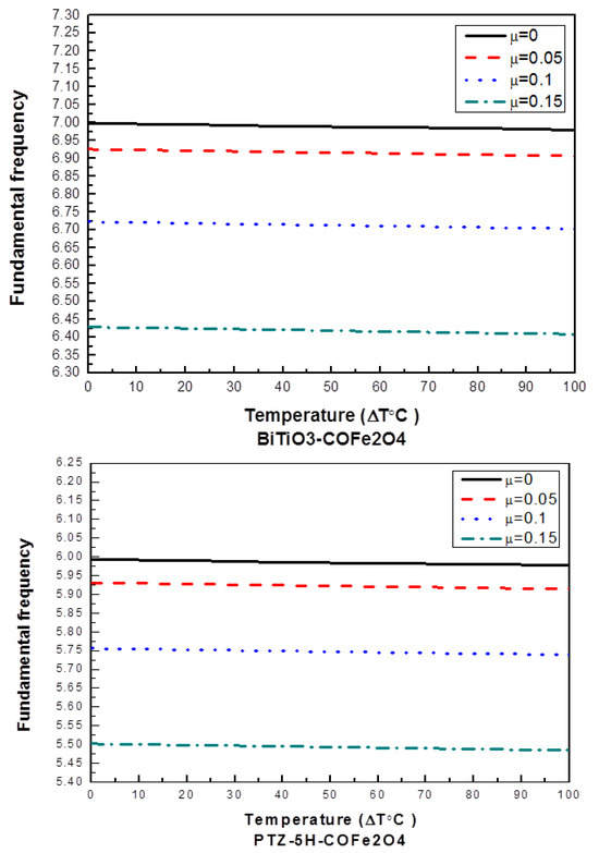
Figure 2.
Impact of temperature and nonlocal parameter on fundamental frequency of hinged–hinged (H-H) METE nanobeam for different materials. ; ; .02; nm; ; ; ; .
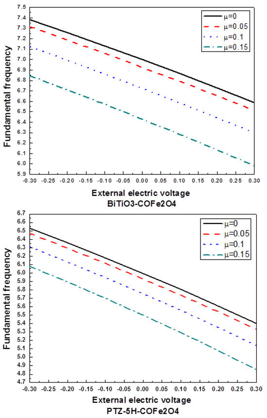
Figure 3.
Impact of electric voltage and nonlocal parameter on fundamental frequency of (H-H) METE nanobeam for different materials. ; ; .02; nm; ; ; ; .
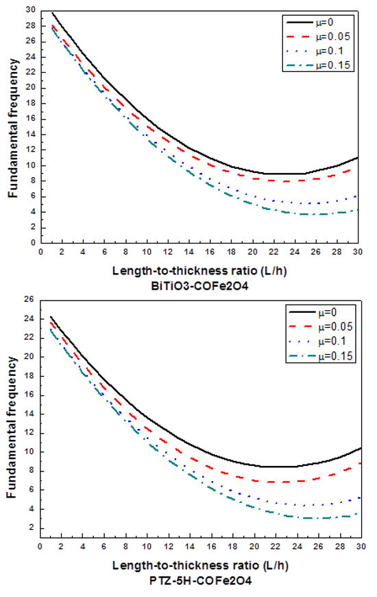
Figure 4.
Impact of length-to-thickness ratio and nonlocal parameter on fundamental frequency of (H-H) METE nanobeam for different materials. ; ; ; ; nm; ; ; .
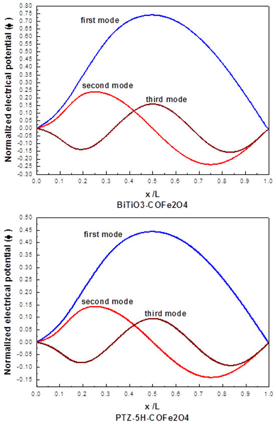
Figure 5.
Electrical potential distribution in (C-C) METE nanobeam for different materials. ; ; ; ; nm; ; .
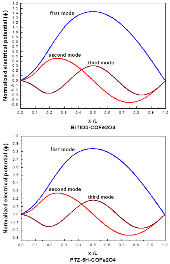
Figure 6.
Electrical potential distribution in (C-C) METE nanobeam for different materials. ; ; ; ; nm; ; ; ; .
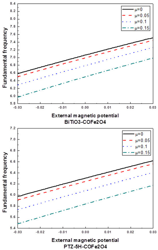
Figure 7.
Impact of magnetic potential and nonlocal parameter on fundamental frequency of (H-H) METE nanobeam for different materials. ; ; .02; nm; ; ; ; .
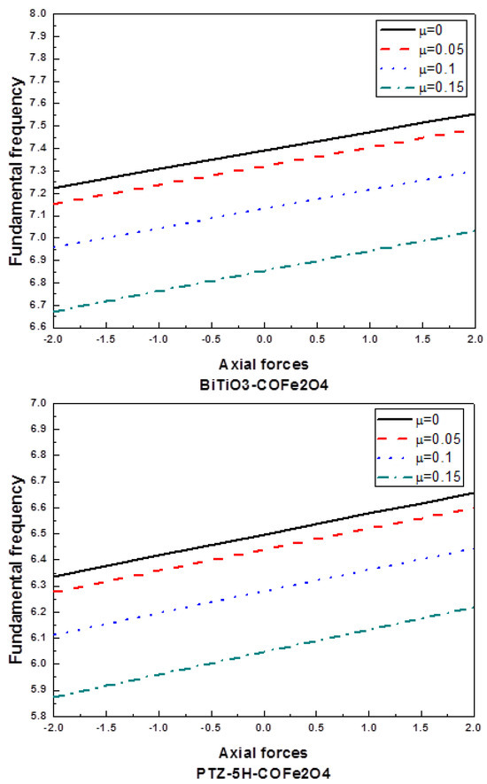
Figure 8.
Impact of axial force and nonlocal parameter on fundamental frequency of (H-H) METE nanobeam for different materials. ; ; .03; nm; ; ; ; .
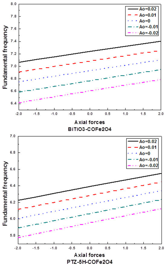
Figure 9.
Impact of axial force and magnetic potential on fundamental frequency of (H-H) METE nanobeam for different materials. ; ; .01; nm; ; ; ; .
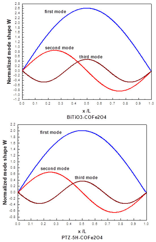
Figure 10.
Mode shapes of (H-H) METE nanobeam for different materials. ; ; ; ; nm; ; .
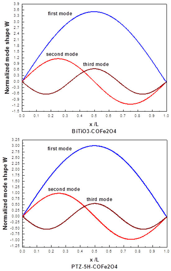
Figure 11.
Mode shapes of (H-H) METE nanobeam for different materials. ; ; ; ; nm; ; ; ; .
The nanobeam’s response was more strongly influenced by the axial force and electric and magnetic fields than by temperature variations. Comparisons between BiTiO3-COFe2O4 and PTZ-5H-COFe2O4 show that the former consistently exhibited a higher fundamental frequency, amplitude, and electric potential. The numerical results, accurate and convergent with other methods, offer valuable design insights for creating customized nanoelectronic and biotechnological smart nanostructures.
5. Discussion
In this section, we introduce the potential advantages and limitations of Ritz methods compared to the DQMs employed in this study: Ritz methods, such as those employing Ritz power series interpolation, often involve simpler discretization procedures compared to DQMs. They typically require fewer grid points, which can lead to reduced computational cost, especially for problems with simple geometries. The use of analytical basis functions, such as polynomials, can provide insights into the analytical behavior of the system and facilitate the understanding of the underlying physics. However, Ritz methods can be challenging to apply to problems with complex geometries or boundary conditions. The convergence of the Ritz method can be sensitive to the choice of basis functions and the number of terms included in the series. Implementing complex material properties, such as those encountered in METE materials, within the Ritz framework can be more intricate than in DQMs. DQMs are highly versatile and can be applied to problems with complex geometries, boundary conditions, and material properties. DQMs can achieve high accuracy with relatively few grid points, making them computationally efficient for many problems. DQMs can be easily adapted to different types of differential equations and boundary conditions. However, the accuracy and convergence of DQM solutions can be sensitive to the choice of grid point distribution. In some cases, DQMs can exhibit numerical instability, particularly for higher-order derivatives. While Ritz methods offer a simpler discretization process, DQMs demonstrate greater versatility and adaptability for handling complex problems encountered in the analysis of METE nanostructures. The choice of the most suitable method depends on the specific characteristics of the problem under consideration, including geometry, boundary conditions, material properties, and computational resources. This brief comparison provides a broader perspective for future readers and encourages the further exploration of alternative numerical techniques for analyzing the dynamics of METE nanostructures.
6. Conclusions
This research provides a highly accurate numerical analysis (error < ) of the vibrational behavior of METE nanobeams, employing three distinct differential quadrature methods (PDQM, Sinc-DQ, and DSCDQM-RSK) implemented via a custom MATLAB program. A parametric study investigated how various factors influence nanobeam vibration, revealing key insights into their behavior:
- The fundamental frequency increased with increasing axial forces, external magnetic potential, and linear elastic foundation characteristics.
- On the other hand, the fundamental frequency decreased when the temperature and the length-to-thickness ratio, nonlocal factors, and external electric voltage increased.
- Increased displacement and electrical potential amplitudes were associated with higher linear (and nonlinear) elastic foundation parameters.
- BiTiO3-COFe2O4 outperformed PTZ-5H-COFe2O4, exhibiting higher fundamental frequency and greater normalized amplitude and electrical potential.
The numerical methods presented accurately and efficiently analyze the dynamic behavior of METE nanobeams. These results are significant for designing and optimizing smart nanostructures with customized properties for nanoelectronics and biotechnology.
Funding
This research received no external funding.
Data Availability Statement
The data presented in this study are available in the article.
Conflicts of Interest
The authors declare no conflicts of interest.
References
- Jandaghian, A.; Jafari, A.; Rahmani, O. Exact solution for Transient bending of a circular plate integrated with piezoelectric layers. Appl. Math. Model. 2013, 37, 7154–7163. [Google Scholar] [CrossRef]
- Nan, C.W. Magneto electric effect in composites of piezoelectric and piezomagnetic phases. Phys. Rev. B 1994, 50, 6082–6088. [Google Scholar] [CrossRef] [PubMed]
- Zhai, J.; Xing, Z.; Dong, S.; Li, J.; Viehland, D. Magnetoelectric laminate composites: An overview. J. Am. Ceram. Soc. 2008, 91, 351–358. [Google Scholar] [CrossRef]
- Nan, C.W.; Bichurin, M.; Dong, S.; Viehland, D.; Srinivasan, G. Multiferroic magnetoelectric composites: Historical perspective, status, and future directions. J. Appl. Phys. 2008, 103, 031101. [Google Scholar] [CrossRef]
- Wu, C.P.; Tsai, Y.H. Static behavior of functionally graded magneto-electro-elastic shells under electric displacement and magnetic flux. Int. J. Eng. Sci. 2007, 45, 744–769. [Google Scholar] [CrossRef]
- Huang, D.J.; Ding, H.J.; Chen, W.Q. Static analysis of anisotropic functionally graded magneto-electro-elastic beams subjected to arbitrary loading. Eur. J. Mech. 2010, 29, 356–369. [Google Scholar] [CrossRef]
- Chang, T.P. Deterministic and random vibration analysis of fluid-contacting transversely isotropic magneto-electro-elastic plates. Comput. Fluids 2013, 84, 247–254. [Google Scholar] [CrossRef]
- Ansari, R.; Gholami, R.; Rouhi, H. Size-dependent nonlinear forced vibration analysis of magneto-electro-thermo-elastic Timoshenko nanobeams based upon the nonlocal elasticity theory. Compos. Struct. 2015, 126, 216–226. [Google Scholar] [CrossRef]
- Ke, L.L.; Wang, Y.S.; Yang, J.; Kitipornchai, S. The size dependent vibration of embedded magneto-electro-elastic cylindrical nanoshells. Smart Mater. Struct. 2014, 23, 125036. [Google Scholar] [CrossRef]
- Prashanthi, K.; Shaibani, P.M.; Sohrabi, A.; Natarajan, T.S.; Thundat, T. Nanoscale magnetoelectric couplinginmultiferroicBiFeO3 nanowires. Phys. Status Solidi R 2012, 6, 244–246. [Google Scholar] [CrossRef]
- Martin, L.W.; Crane, S.P.; Chu, Y.H.; Holcomb, M.B.; Gajek, M.; Huijben, M.; Yang, C.H.; Balke, N.; Ramesh, R. Multiferroic and magnetoelectrics: Thin films and nanostructures. J. Phys. Condens. Matter. 2008, 20, 434220. [Google Scholar] [CrossRef]
- Akgöz, B.; Civalek, O. Buckling analysis of cantilever carbon nanotubes using the strain gradient elasticity and modified couple stress theories. J. Comput. Theor. Nanosci. 2011, 8, 1821–1827. [Google Scholar] [CrossRef]
- Li, C. A nonlocal analytical approach for torsion of cylindrical nanostructures and the existence of higher-order stress and geometric boundaries. Compos. Struct. 2014, 118, 607–621. [Google Scholar] [CrossRef]
- Shen, Z.B.; Li, X.F.; Sheng, L.P.; Tang, G.J. Transverse vibration of nanotube-based micro-mass sensor via nonlocal Timoshenko beam theory. Comput. Mater. Sci. 2012, 53, 340–346. [Google Scholar] [CrossRef]
- Li, X.F.; Wang, B.L. Vibrational modes of Timoshenko beams at small scales. Appl. Phys. Lett. 2009, 94, 101903. [Google Scholar] [CrossRef]
- Huang, Y.; Luo, Q.Z.; Li, X.F. Transverse waves propagating in carbon nanotubes via a higher-order nonlocal beam model. Compos. Struct. 2013, 95, 328–336. [Google Scholar] [CrossRef]
- Shen, J.P.; Li, C. A semi-continuum-based bending analysis for extreme-thin micro/nano-beams and new proposal for nonlocal differential constitution. Compos. Struct. 2017, 172, 210–220. [Google Scholar] [CrossRef]
- Mercan, K.; Civalek, O. DSC method for buckling analysis of boron nitride nanotube (BNNT) surrounded by an elastic matrix. Compos. Struct. 2016, 143, 300–309. [Google Scholar] [CrossRef]
- Şimşek, M.; Yurtcu, H. Analytical solutions for bending and buckling of functionally graded nan obeams based on the nonlocal Timoshenko beam theory. Compos. Struct. 2013, 97, 378–386. [Google Scholar] [CrossRef]
- Arefi, M.; Zenkour, A.M. A simplified shear and normal deformations nonlocal theory for bending of functionally graded piezomagnetic sandwich nanobeams in magneto-thermo-electric environment. J. Sandw. Struct. Mater. 2016, 18, 624–651. [Google Scholar] [CrossRef]
- Jian, S.P.; Yan, L.; Jie, Y. A Semi Analytical Method for Nonlinear Vibration of Euler-Bernoulli Beams with General Boundary Conditions. Math. Probl. Eng. 2010, 2010, 591786. [Google Scholar] [CrossRef]
- Norouzzadeh, A.; Ansari, R. Finite element analysis of nano-scale Timoshenko beams using the integral model of nonlocal elasticity. Phys E. 2017, 88, 194–200. [Google Scholar] [CrossRef]
- Roque, C.M.C.; Fidalgo, D.S.; Ferreira, A.J.M.; Reddy, J.N. A study of a microstructure-dependent composite laminated Timoshenko beam using a modified couple stress theory and a meshless method. Compos. Struct. 2013, 96, 532–537. [Google Scholar] [CrossRef]
- Foroughi, H.; Azhari, M. Mechanical buckling and free vibration of thick functionally graded plates resting on elastic foundation using the higher order B-spline finite strip method. Meccanica 2014, 49, 981–993. [Google Scholar] [CrossRef]
- Fakher, M.; Shahrokh, H.H. Bending and free vibration analysis of nanobeams by differential and integral forms of nonlocal strain gradient with Rayleigh–Ritz method. Mater. Res. Express 2017, 4, 125025. [Google Scholar] [CrossRef]
- Sizikov, V.; Sidorov, D. Generalized quadrature for solving singular integral equations of Abel type in application to infrared tomography. Appl. Numer. Math. 2016, 106, 69–78. [Google Scholar] [CrossRef][Green Version]
- Ragb, O.; Mohamed, M.; Matbuly, M.S.; Civalek, O. Nonlinear Analysis of Organic Polymer Solar Cells Using Differential Quadrature Technique with Distinct and Unique Shape Function. CMES-Comput. Model. Eng. Sci. 2023, 137, 8992. [Google Scholar] [CrossRef]
- Mohamed, M.; Mabrouk, S.M.; Rashed, A.S. Mathematical investigation of the infection dynamics of COVID-19 using the fractional differential quadrature method. Computation 2023, 10, 198. [Google Scholar] [CrossRef]
- Ragb, O.; Wazwaz, A.M.; Mohamed, M.; Matbuly, M.S.; Salah, M. Fractional differential quadrature techniques for fractional order Cauchy reaction-diffusion equations. Math. Methods Appl. Sci. 2023, 9, 10216–10233. [Google Scholar] [CrossRef]
- Mustafa, A.; Ragb, O.; Salah, M.; Salama, R.S.; Mohamed, M. Distinctive Shape Functions of Fractional Differential Quadrature for Solving Two-Dimensional Space Fractional Diffusion Problems. Fractal Fract. 2023, 9, 668. [Google Scholar] [CrossRef]
- Shojaei, M.F.; Ansari, R. Variational differential quadrature: A technique to simplify numerical analysis of structures. Appl. Math. Model. 2017, 49, 705–738. [Google Scholar] [CrossRef]
- Tornabene, F.; Fantuzzi, N.; Viola, E.; Carrera, E. Static analysis of doubly-curved anisotropic shells and panels using CUF approach, differential geometry and differential quadrature method. Compos. Struct. 2014, 107, 675–697. [Google Scholar] [CrossRef]
- Tornabene, F.; Dimitri, R.; Viola, E. Transient dynamic response of generally shaped arches based on a GDQ-Time-stepping method. Int. J. Mech. Sci. 2016, 114, 277–314. [Google Scholar] [CrossRef]
- Korkmaz, A.; İdris, D. Shock wave simulations using Sinc Differential Quadrature Method. Eng. Comput. Int. J. Comput. Aided Eng. Softw. 2011, 28, 654–674. [Google Scholar] [CrossRef]
- Ke, L.L.; Wang, Y.S.; Wang, Z.D. Nonlinear vibration of the piezoelectric nanobeams based on the nonlocal theory. Compos. Struct. 2012, 94, 2038–2047. [Google Scholar] [CrossRef]
- Civalek, O.; Kiracioglu, O. Free vibration analysis of Timoshenko beams by DSC method. Int. J. Numer. Meth. Biomed. Engng. 2010, 26, 250–275. [Google Scholar] [CrossRef]
- Seçkin, A.; Sarıgül, A.S. Free vibration analysis of symmetrically laminated thin composite plates by using discrete singular convolution (DSC) approach: Algorithm and verification. J. Sound Vib. 2009, 315, 197–211. [Google Scholar] [CrossRef]
- Civalek, O. Free vibration of carbon nanotubes reinforced (CNTR) and functionally graded shells and plates based on FSDT via discrete singular convolution method. Compos. Part B 2017, 111, 45–59. [Google Scholar] [CrossRef]
- Civalek, O. Vibration analysis of conical panels using the method of discrete singular convolution. Commun Numer. Methods Eng. 2008, 24, 169–181. [Google Scholar] [CrossRef]
- Ragb, O.; Mohamed, M.; Matbuly, M.S.; Civalek, O. Sinc and discrete singular convolution for analysis of three-layer composite of perovskite solar cell. Int. J. Energy Res. 2022, 46, 4279–4300. [Google Scholar] [CrossRef]
- Jandaghian, A.A.; Rahmani, O. Free vibration analysis of magneto-electrothermo elastic nanobeams resting on a Pasternak foundation. Smart Mater. Struct. 2016, 25, 035023. [Google Scholar] [CrossRef]
- Chang, S. Differential Quadrature and Its Application in Engineering; Springer-Verlag London Ltd.: London, UK, 2000. [Google Scholar] [CrossRef]
- Mustafa, A.; Salama, R.S.; Mohamed, M. Semi-Analytical Analysis of Drug Diffusion through a Thin Membrane Using the Differential Quadrature Method. Mathematics 2023, 11, 2998. [Google Scholar] [CrossRef]
- Abdelfattah, W.M.; Ragb, O.; Salah, M.; Mohamed, M. A Robust and Versatile Numerical Framework for Modeling Complex Fractional Phenomena: Applications to Riccati and Lorenz Systems. Fractal Fract. 2024, 8, 647. [Google Scholar] [CrossRef]
- Shashidhar, S.; Jiang, L.Y. The effective magnetoelectric coefficients of polycrystalline multiferroic composites. Acta Mater. 2005, 53, 4135–4142. [Google Scholar] [CrossRef]
- Jandaghian, A.A.; Rahmani, O. An analytical Solution for Free Vibration of Piezoelectric nanobeams Based on a Nonlocal Elasticity Theory. Smart Mater. Struct. 2016, 32, 143–151. [Google Scholar] [CrossRef]
- Ke, L.-L.; Wang, Y.-S. Free vibration of size dependent magneto-electro-elastic nanobeams based on the nonlocal theory. Phys. E 2014, 63, 52–61. [Google Scholar] [CrossRef]


Disclaimer/Publisher’s Note: The statements, opinions and data contained in all publications are solely those of the individual author(s) and contributor(s) and not of MDPI and/or the editor(s). MDPI and/or the editor(s) disclaim responsibility for any injury to people or property resulting from any ideas, methods, instructions or products referred to in the content. |
© 2025 by the author. Licensee MDPI, Basel, Switzerland. This article is an open access article distributed under the terms and conditions of the Creative Commons Attribution (CC BY) license (https://creativecommons.org/licenses/by/4.0/).