Beyond Spectrograms: Rethinking Audio Classification from EnCodec’s Latent Space

Abstract

This paper presents a novel approach to audio classification leveraging the latent representation generated by Meta’s EnCodec neural audio codec. We hypothesize that the compressed latent space representation captures essential audio features more suitable for classification tasks than the traditional spectrogram-based approaches. We train a vanilla convolutional neural network for music genre, speech/music, and environmental sound classification using EnCodec’s encoder output as input to validate this. Then, we compare its performance training with the same network using a spectrogram-based representation as input. Our experiments demonstrate that this approach achieves comparable accuracy to state-of-the-art methods while exhibiting significantly faster convergence and reduced computational load during training. These findings suggest the potential of EnCodec’s latent representation for efficient, faster, and less expensive audio classification applications. We analyze the characteristics of EnCodec’s output and compare its performance against traditional spectrogram-based approaches, providing insights into this novel approach’s advantages.

1. Introduction

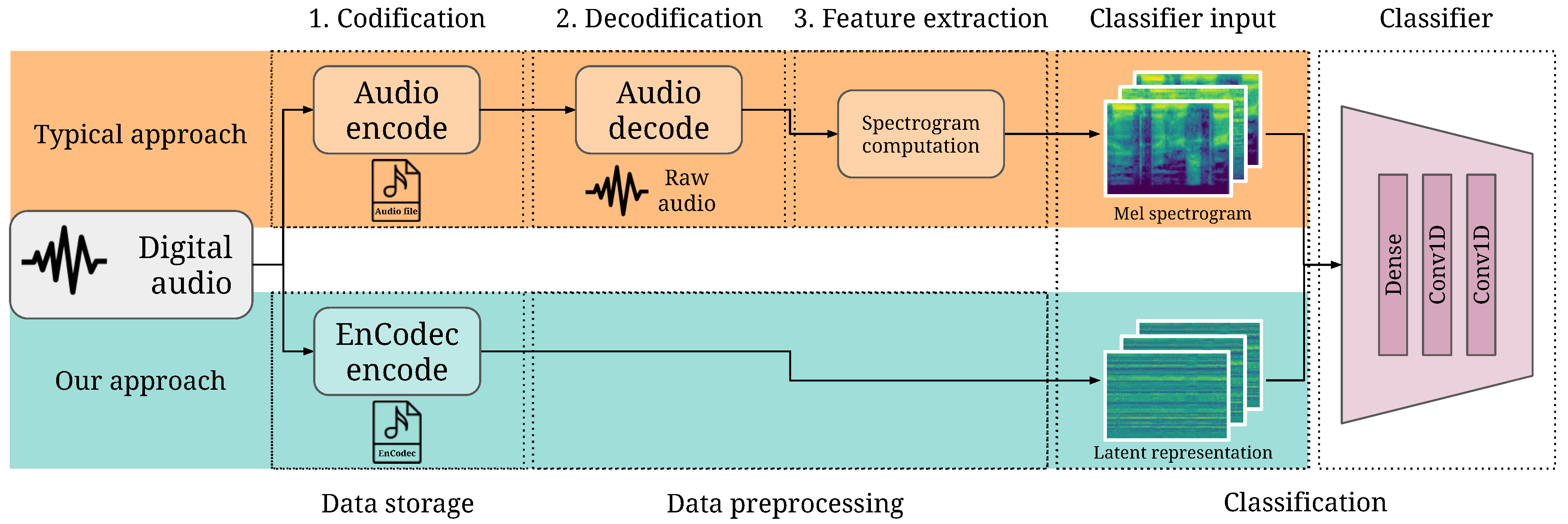
The content we consume today, both for our education and leisure, has undergone a radical change in recent years, becoming mostly multimedia. Within this content, audio is one of the most important sources, whether in music, podcasts, audiobooks, or as part of an audiovisual product. Audio compression and classification are two essential tasks in the audio processing pipeline, as shown in Figure 1.

Audio compression is crucial, enabling efficient audio content storage, transmission, and playback. By reducing the size of audio files, compression allows for significant storage savings. This is particularly important in an era where vast amounts of audio content are consumed and stored. Furthermore, compression facilitates faster and more reliable audio transmission over the Internet and wireless networks, as compressed audio files require less bandwidth, reducing download times. Due to its widespread compatibility, relatively high compression ratio, and acceptable audio quality for most listeners, MP3 has become a de facto standard for music distribution and download [1]. Streaming services like Apple Music and Spotify use AAC. While AAC offers superior audio quality compared to MP3 at similar bit rates, MP3 remains the most popular audio format for distribution and download.

Although MP3 is the de facto standard, its replacement by another format offering significant advantages is not unreasonable. This transition would be transparent to the user, considering its use is usually made through an intermediary, such as a web client, a music application, or a video player, to mention a few examples.

Audio classification is used in various applications, such as categorizing audio content, enhancing music recommendation systems, automating metadata tagging, and aiding copyright detection in the music industry. It also plays a crucial role in music segmentation for production, facilitating research through trend analysis and improving sound engineering processes. The integration of technology and music optimizes industry workflows, enriches the user experience, and protects intellectual property. The scientific community has addressed the task of extracting the different features that an audio track may have for decades. Audio classification techniques were traditionally solved by extracting and processing audio features using probabilistic analysis. Some libraries, such as pyAudioAnalysis [2], Essentia [3], or librosa [4], allow audio feature extraction. However, adopting Artificial Intelligence (AI) techniques has revolutionized audio classification, allowing the task to be performed without requiring manual feature extraction. This made pyAudioAnalysis one of the first libraries to incorporate AI techniques for audio classification. Spectrogram-related features are the most widely used in AI audio classification tasks, as they provide a good representation of the audio signal’s frequency content over time.

A new audio compression algorithm, named EnCodec, has been recently proposed [5]. EnCodec is a neural audio codec that uses a streaming encoder–decoder architecture with quantized latent space to achieve high-fidelity audio compression in real-time. It provides up to 10 times less bandwidth than MP3 while maintaining the same audio quality.

However, EnCodec is not the only neural audio codec of its kind, as this technology has gained significant research interest among major tech companies. Google’s SoundStream [6] operates similarly to EnCodec, utilizing an encoder–decoder architecture that produces a latent representation of audio samples, which is then quantized using Residual Vector Quantization (RVQ). Nevertheless, EnCodec achieves a higher Multiple Stimuli with Hidden Reference and Anchor (MUSHRA) (https://www.itu.int/rec/R-REC-BS.1534/en, accessed on 1 February 2025) score ($53.1$ vs. 67 for 3 $\mathrm{kbit}$/$\mathrm{s}$ and $66.2$ vs. $83.1$ for 6 $\mathrm{kbit}$/$\mathrm{s}$). Similarly, NVIDIA’s NeMo Mel Codec [7] achieves the same objective by encoding disjoint mel-bands separately and quantizing them using Finite Scalar Vector Quantization (FSQ). All codebook embeddings are then concatenated and fed into a HiFi-GAN [8] decoder, which reconstructs the final waveform. Meta has also released AudioDec [9], an open-source, high-fidelity neural audio codec designed for streaming. It utilizes SoundStream as the codec along with HiFi-GAN neural vocoder. The authors argue that combining a robust vocoder with a well-trained encoder results in the highest audio quality. AudioDec is particularly optimized for real-time applications, and they also propose an efficient training paradigm. Finally, SNAC, a multi-scale neural audio codec [10], employs multi-scale RVQ instead of the traditional RVQ approach. In conventional RVQ, tokens are generated at a fixed temporal resolution, whereas SNAC utilizes a hierarchy of quantizers operating at multiple temporal resolutions. This design allows the codec to capture both coarse and fine audio details more effectively.

This paper proposes a novel approach to audio classification using EnCodec, which simplifies and improves the classification process. We hypothesize that EnCodec’s latent representation of audio signals can be used to classify audio signals more efficiently than spectrogram-based classification techniques. In addition, the computational load of the training process gets reduced, as the latent representation is more suited for this kind of task because of its reduced size and better data representation. In order to prove this hypothesis, we demonstrate that (1) the network converges on the same or fewer epochs using the EnCodec latent representation rather than the spectrogram, (2) the accuracy obtained using the latent EnCodec representation is better than that obtained using the spectrogram with the same epochs, and (3) after training, classifying with EnCodec is faster than with the spectrogram.

2. Methodology

EnCodec’s architecture contains several components: an encoder, a quantizer, and a decoder. The encoder part of EnCodec is based on SEANet [11] and takes a raw audio sample as input. It converts it into a compressed latent representation using convolutional layers and a Long Short-Term Memory (LSTM) network through a series of steps. The audio signal first passes through a 1D convolution layer with 32 channels and a kernel size of 7, extracting the audio’s initial features. After the initial convolution, the output is passed through four convolution blocks, each consisting of a residual unit and a downsampling layer. The residual unit helps to learn complex relationships between the features. At the same time, the downsampling layer reduces the dimensionality of the latent space. After the convolution blocks, a two-layer LSTM network is used to model the temporal dependencies in the latent representation to capture the time-varying nature of the audio signal. Finally, a 1D convolution layer with a kernel of size seven and a variable number of output channels is applied. The number of output channels depends on the target bit rate for the compressed audio. The encoder’s output is a latent representation of the audio signal that is smaller in size than the original audio. This latent representation is then quantized and further compressed using entropy coding before being transmitted or stored.

The quantizer then processes the encoder output. Its objective is to reduce the bit rate of the compressed audio signal while minimizing the loss of perceptual quality using RVQ [6], reducing the dimensionality of the latent representation. Using the quantizer output for audio classification could be an exciting approach. It could be easier and faster to process as it is smaller than the raw audio signal. However, more than this output is required to classify the audio signal, as there is no direct relationship between the quantized values and the audio signal’s content.

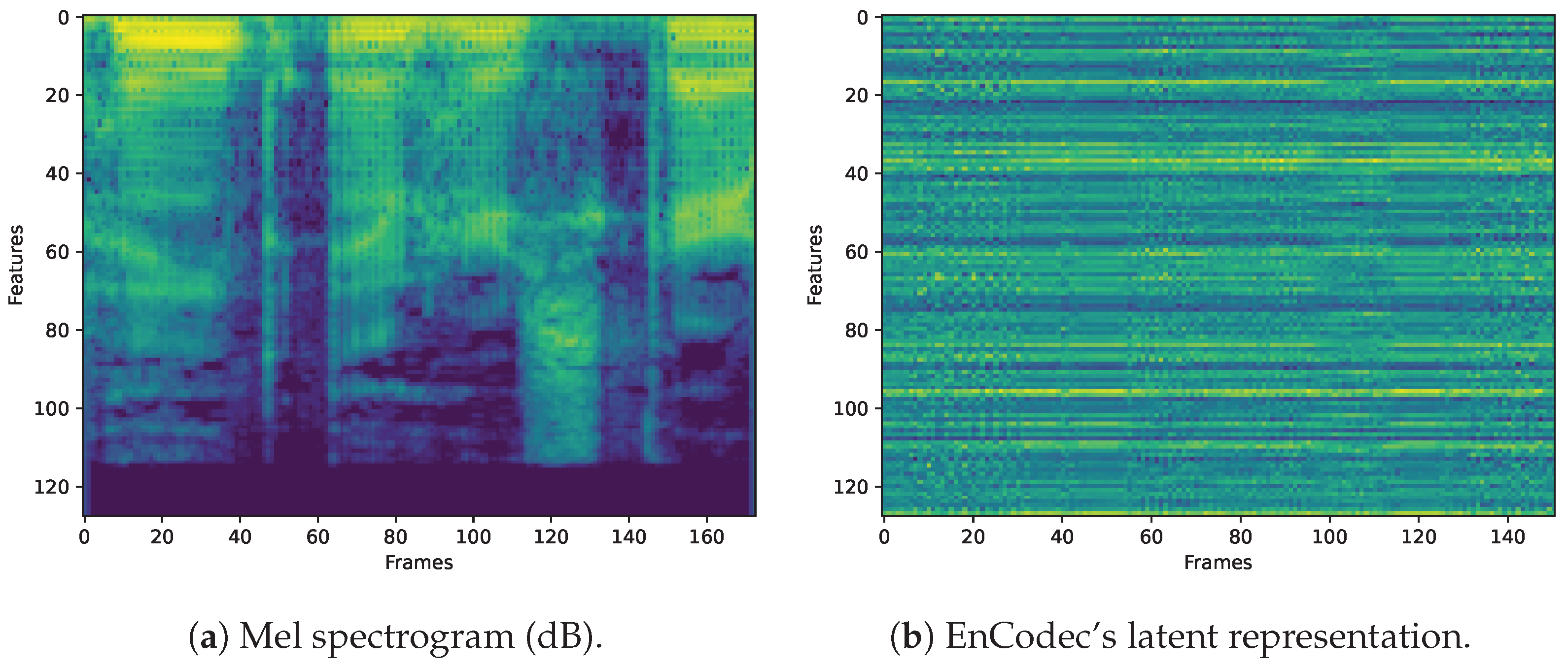
A 1-s mel spectrogram representation from a sample speech audio (Ashiel Mystery, A Detective Story, Ch. 2: https://librosa.org/doc/main/recordings.html#description-of-examples, accessed on 1 February 2025) is shown in Figure 2a. The mel spectrogram is widely used in AI audio classification tasks. It is included as a layer in Keras 3.1 (https://keras.io/, accessed on 1 February 2025) or as an output format in Kapre [12]. Unlike linear spectrograms, mel spectrograms use a frequency scale that mimics the human ear’s sensitivity. They also outperform Short-time Fourier transform (STFT), as the resulting images are more compact. This makes them particularly effective in tasks involving audio analysis, such as speech and music processing. This approach has been widely adopted in the literature [13], demonstrating its effectiveness in audio classification tasks. For comparison, Figure 2b shows the encoder’s output after processing the same sample but before the quantization, obtained from EnCodec’s 48 $\mathrm{k}$$\mathrm{Hz}$ model. A naked-eye inspection of the visual patterns of EnCodec latent representation compared to the mel spectrogram clearly shows a reorganization of the data. The output of the EnCodec’s encoder reduces the size of the audio and reorganizes it to facilitate its subsequent compression. We hypothesize that such reorganization may also be useful for audio classification, even though the encoder’s output appears to be noise if played back as an audio signal. The nature of the audio signal is still present in EnCodec’s encoder output in a way that is not directly perceptible to the human ear but that a neural network could learn to recognize.

To test this paper’s hypothesis, we trained an EnCodec-based audio classifier built on a neural network architecture (https://keras.io/examples/vision/mnist_convnet/, accessed on 1 February 2025) based on the Modified National Institute of Standards and Technology (MNIST) (https://web.archive.org/web/20250112235228/http://yann.lecun.com/exdb/mnist/, accessed on 1 February 2025) classifier. The diagram in Figure 1 illustrates the relationship between the classifier and the entire system. The input layer is an array of $128\times X$ obtained after preprocessing the audio samples, passing through convolutional and pooling layers. Input layer size, 128, is chosen to match the output size of EnCodec’s encoder or the number of mel bands chosen to compute the mel spectrogram. X depends on the length of the computed frame and the preprocessing step (e.g., 150 items for 1 s of stereo 48 $\mathrm{k}$$\mathrm{Hz}$ EnCodec compression or 75 items for 1 s of mono 24 $\mathrm{k}$$\mathrm{Hz}$) EnCodec compression. It is also variable depending on the number of samples between successive frames when computing the mel spectrogram (e.g., 173 when using 256 as the hop length for a 44.1 kHz audio).

Once the audio file is loaded, it is represented as a vector of length $N\times SR$, where N is the duration of the audio in seconds and $SR$ is the sampling rate. In the case of multi-channel audio, such as stereo files, the representation takes the form of a matrix with dimensions ($NC$, $N\times SR$), where $NC$ is the number of channels and $N\times SR$ corresponds to the number of samples per channel.

For the calculation of the mel spectrogram, the first step in our process is to convert the multi-channel audio to mono format. This is achieved by averaging the values across all channels, thereby reducing dimensionality and facilitating subsequent processing. Once converted to mono, the audio is segmented into fragments of $WINDOW$ seconds using a sliding window that advances $STEP$ seconds between each segment. This approach generates a series of uniform-sized segments that are used for model training and prediction.

The result of this process is a set of segments represented as a vector with dimensions (M, $WINDOW\times SR$), where M is the total number of segments generated. Each segment corresponds to a specific fragment of the audio that is processed individually by the neural network. This methodology enables not only the classification of the entire audio file but also its precise segmentation, which is particularly useful for analyzing changes within a single track.

The process of audio segmentation using a sliding window can be described as follows. In this example, an audio file with a duration of 10 s is used, and a sliding window with a length of $WINDOW=2$ s and a step of $STEP=1$ s is applied. Since the window size is twice the step size, there is overlap between adjacent fragments, which is advantageous for preventing the loss of critical information. The first window fragment will capture the audio interval $[0,2]$, while the second will capture the range $[1,3]$, and so on. This overlap ensures that audio elements near the edges of each window are not left unprocessed, which is crucial in situations where changes in the audio occur gradually. For the final window segment, padding is applied using NumPy functions. Instead of assigning silence values, this padding replicates the audio content in an inverted manner, which helps to prevent potential bias in the model. This approach is particularly important in scenarios where pauses or silence are treated as distinct classes for classification. Assigning artificial silence could interfere with the accurate differentiation of speech and non-speech segments, as natural pauses should be preserved to ensure the model correctly distinguishes between speech and pauses without artificial influence.

The model incorporates a preprocessing layer that transforms the segmented fragments into images through the mel spectrogram representation. This representation is obtained using a 512-frames Hamming window, equivalent to 25 $\mathrm{m}$$\mathrm{s}$, with a hop size of 128 samples, and 128 mel bins. The final shape of these images is computed using the expression described in (1):

$$\left(W,H\right)=\left(⌊{\displaystyle \frac{(sample\_rate\times window)-stft\_win\_length}{stft\_hop\_length}}⌋+1,stft\_n\_mels\right)$$

(1)

where $W,H$ are the width and the height of the resulting image, respectively.

Conversely, in the case of preprocessing with EnCodec, a different strategy is followed. Instead of converting the audio to mono format and generating the mel spectrogram, the audio file is first fully compressed using this system. This compression provides a more compact representation in the form of an array with dimensions $(128, 75\times N)$ for EnCodec mono at 24 $\mathrm{k}$$\mathrm{Hz}$, and $(128, 150\times N)$ for EnCodec stereo at 48 $\mathrm{k}$$\mathrm{Hz}$, where N represents the duration of the audio in seconds.

However, this compressed representation also requires additional processing. Once the compression is obtained, a sliding window is applied to the resulting array, similar to the mel spectrogram approach. The new representation takes the form $(N/WINDOW,$ $128, 75\times WINDOW)$ for the EnCodec mono case and $(N/WINDOW,128, 150\times WINDOW)$ for EnCodec stereo. This means that the compressed audio is segmented into fixed-size fragments, where each fragment contains $WINDOW$ seconds of information.

Unlike the mel spectrogram, the EnCodec approach leverages the compressed information directly, reducing the size of the data to be processed, which can be advantageous in scenarios where computational efficiency is a priority. However, this strategy may sacrifice some of the spectral detail present in the mel spectrogram, which could impact the model’s performance depending on the specific task. Thus, the choice between one method or the other will depend on the balance between compression, efficiency, and the quality of the represented information.

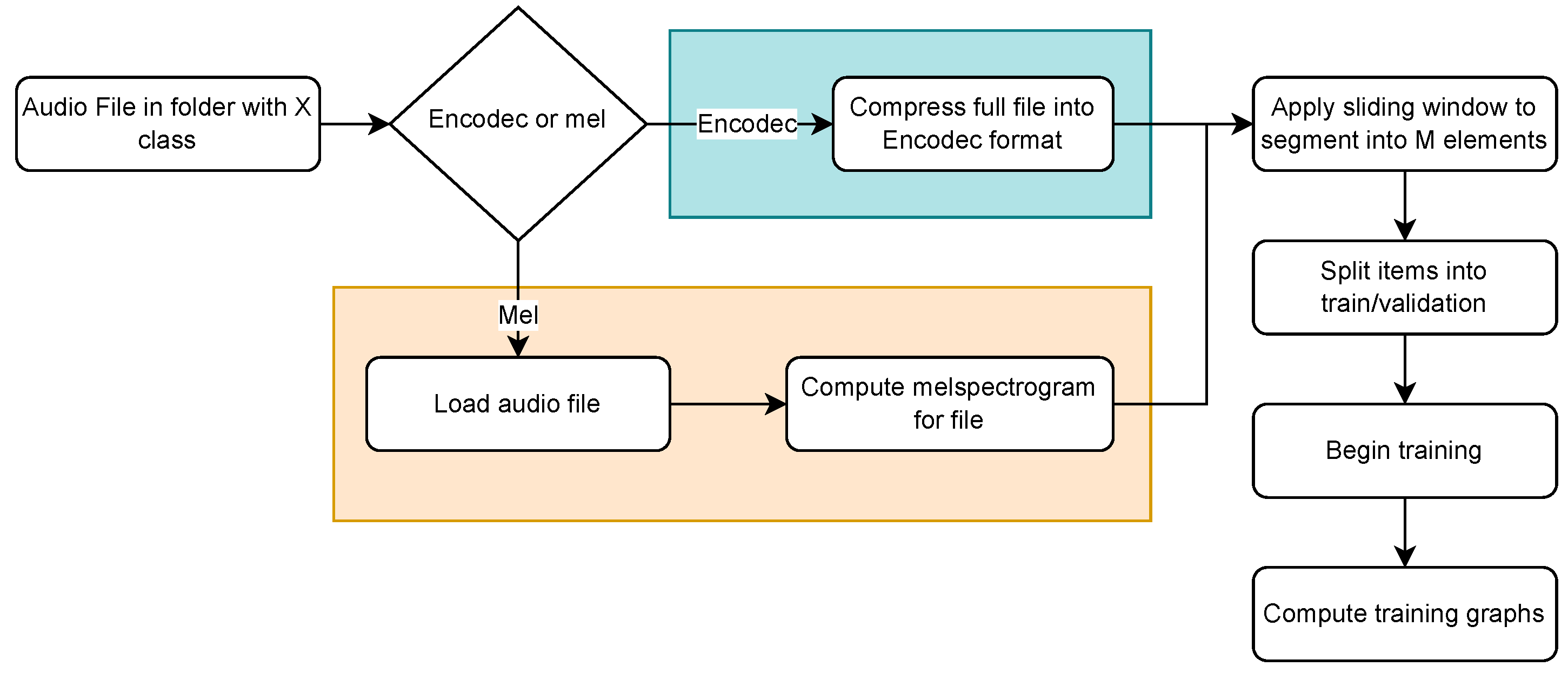
To simplify the data loading process during model training and evaluation, an efficient process has been designed to streamline the loading and organization of audio data for deep learning tasks. This process automatically assigns the folder name containing each file as its class, thereby simplifying the data structure and eliminating the need for separate label files.

The method organizes audio files into folders, with each folder named after the class of the files it contains, simplifying preprocessing, reducing errors, and speeding up data loading, especially for large datasets. An automated script iterates through the folders, identifies files in formats such as WAV, MP3, or FLAC, and assigns the corresponding label, while validating file properties such as sampling rate and duration, among others.

This approach simplifies audio classification experiments and is adaptable to other scenarios such as speaker identification or sound event detection. Additionally, it allows for the scalable addition of new classes by incorporating additional folders into the dataset. Figure 3 illustrates how these processes operate depending on the type of algorithm used for model creation.

The output layer of the neural network is a softmax layer with a series of nodes, each representing a different audio class. This output layer will have two nodes if the classification task is binary (e.g., speech or music in the GTZAN music/speech dataset [14]). If the classification task is multi-class (e.g., music genres in the GTZAN genres dataset [15]), the output layer will have ten nodes, one for each genre. The proposed network is trained with three different data sources. First, it uses the mel spectrogram obtained after loading the audio file and processing the raw audio signal. Then, it uses EnCodec’s intermediate latent representation as input (both in 24 and 48 $\mathrm{k}$$\mathrm{Hz}$), which can be obtained directly from EnCodec’s compressed audio.

3. Experiments

In this paper, we have performed a series of experiments to evaluate the performance of a classification system using EnCodec’s latent representation as input. Although the chosen MNIST architecture does not achieve the best results, it is simple and well-known, making the results easier to understand. Furthermore, if a network such as the one used in this work can obtain results comparable to those of more complex networks, it could be concluded that EnCodec’s latent representation is adequate for the audio classification task. Any network architecture capable of performing classification tasks could be used to achieve similar results. In contrast, more complex networks would improve the results.

In each experiment, three different inputs generated from the original audio have been used: the mel spectrogram, the output of the EnCodec encoder at 48 $\mathrm{k}$$\mathrm{Hz}$, and the output of the EnCodec encoder at 24 $\mathrm{k}$$\mathrm{Hz}$. To ensure that the same results are obtained with data of different natures, these experiments have been performed with three different datasets: the GTZAN music/speech dataset [14], the GTZAN music genres dataset [15], and the ESC-50 environmental sound dataset [16]. These experiments determine whether the proposed system’s results are better than those of other audio classification systems. For this purpose, the classification accuracy and the number of epochs needed to reach convergence will be compared. In addition, other characteristics of the result, such as the size of the analyzed samples, will be examined.

Let us compare the size of 1 s taken from the samples used in this work in three different formats: its mel spectrogram representation, and the 48 $\mathrm{k}$$\mathrm{Hz}$ and 24 $\mathrm{k}$$\mathrm{Hz}$ intermediate representation EnCodec’s encoder produces. If our hypothesis is correct, although the mel spectrogram representation is the largest, EnCodec’s 48 $\mathrm{k}$$\mathrm{Hz}$ and 24 $\mathrm{k}$$\mathrm{Hz}$ intermediate latent representations could provide better results, even with a smaller size. There are differences when comparing the size of 1 s taken from the samples in the three formats used in this work. Its mel spectrogram representation consists of 173 items, EnCodec’s 48 $\mathrm{k}$$\mathrm{Hz}$ intermediate representation consists of 150 items (13.29% less), and EnCodec’s 24 $\mathrm{k}$$\mathrm{Hz}$ intermediate representation consists of 75 items (56.65% less).

3.1. Experimental Environment

Several experiments have been conducted to evaluate the performance of the EnCodec-based audio classification model proposed in this work. These have been run on a hardware platform equipped with an AMD Ryzen 9 3900X 12-Core processor with 64 GB of DDR4 RAM, an NVidia RTX 3060 with 12 GB of GDDR6 VRAM, and CUDA version 11.8.

The GTZAN music/speech [14], GTZAN musical genres [15], and ESC-50 environmental sound [16] datasets have been chosen for the experiments. The first one, used for two-class audio classification (music and speech), contains 64 samples per class of 30 s each. The second one, with an original frame rate of 22,050 Hz, contains 100 samples per class of 30 s each for ten different musical genres in the dataset, making it a total of 1000 items and 30,000 s of audio. The third is a labeled collection of 2000 environmental audio recordings suitable for benchmarking methods of environmental sound classification. The dataset consists of 5 -s recordings organized into 50 semantic classes.

We have chosen 1 -s item patches without overlapping and divided the dataset into training (60%), evaluation (20%), and test (20%). The input signal from these datasets is always monoaural. EnCodec at 48 $\mathrm{k}$$\mathrm{Hz}$ is stereo, while EnCodec at 24 $\mathrm{k}$$\mathrm{Hz}$ is monoaural. In order to transform the samples to stereo, the signal is duplicated in both channels. This conversion does not add any information to the signal. However, it is necessary for EnCodec to work with the audio information. Although EnCodec is used as-is, only the encoder part is needed, leaving out the quantizer and decoder parts. The framework’s source code was implemented with the PyTorch 2.1.0 library on Python 3.11.4.

3.2. Results

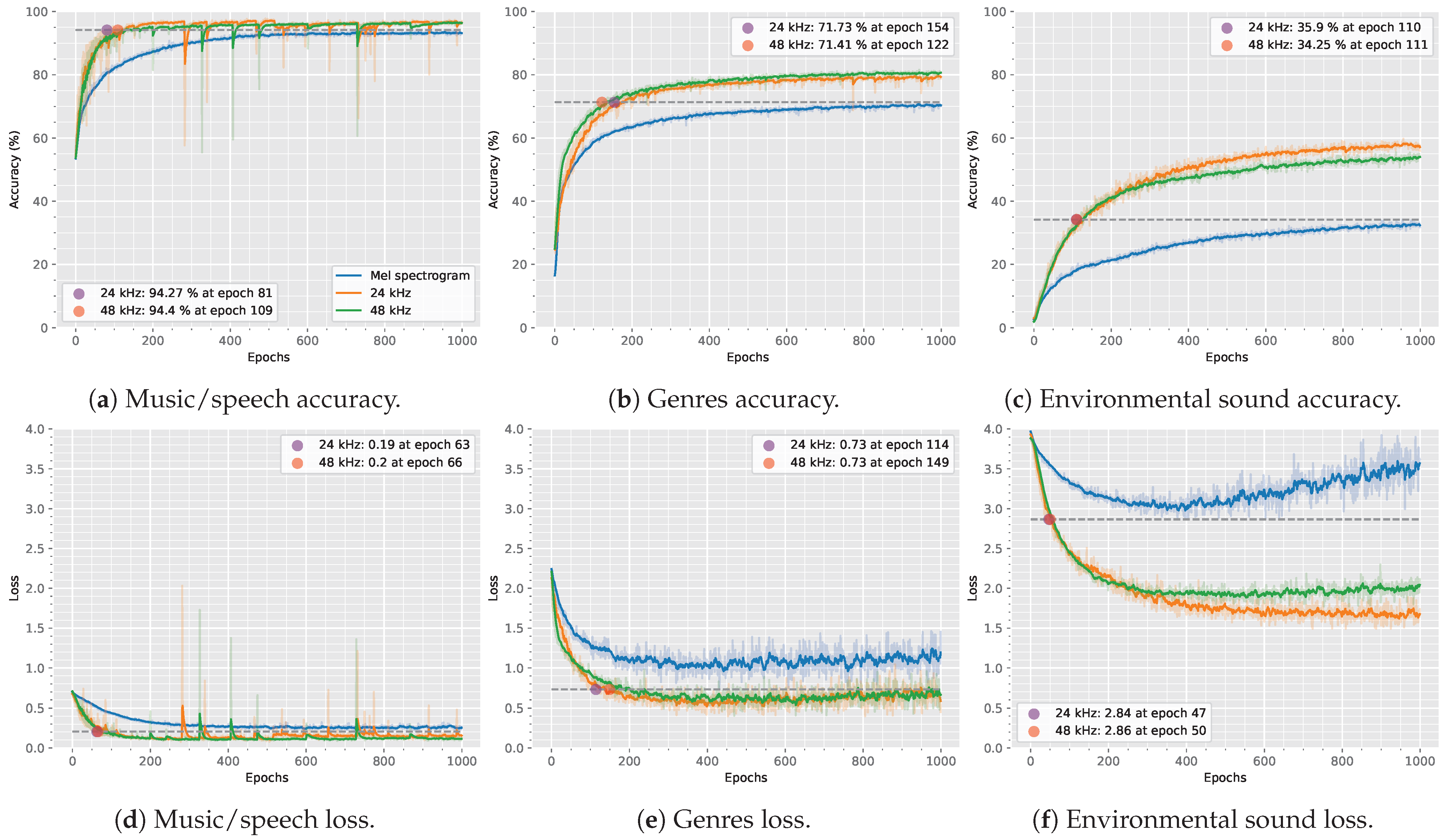
Figure 4 shows the result of the training process of the audio classification models based on EnCodec, in its versions of 24 $\mathrm{k}$$\mathrm{Hz}$ and 48 $\mathrm{k}$$\mathrm{Hz}$, compared to those obtained using the mel spectrogram of the signal. The blue line represents the mel spectrogram, the orange line corresponds to the 24 $\mathrm{k}$$\mathrm{Hz}$ EnCodec version, and the green line represents the 48 $\mathrm{k}$$\mathrm{Hz}$ EnCodec version. All lines are smoothed with a $0.8$ factor for better visualization. Additionally, the original unsmoothed lines are displayed in the same colors with reduced opacity for reference. Figure 4a,d show the evolution of accuracy and loss values using the music/speech dataset, respectively. On the other hand, the evolution of accuracy and loss using the music genres dataset is shown in Figure 4b and Figure 4e, respectively. Finally, Figure 4c,f show the evolution of accuracy and loss using the environmental sound dataset.

The developed system learns to classify speech and music, music genres, and environmental sound better (i.e., with higher accuracy and lower loss) using EnCodec latent representation, compared with the mel spectrogram. Moreover, it reaches values close to the maximum accuracy and minimum loss much earlier (in fewer epochs) than the mel spectrogram-based model. All experiments run for 1000 epochs.

Let us look at speech and music classification at epochs 81/109. The proposed system obtains better results with EnCodec’s latent representation than the mel spectrogram-based model at the end of the run (94.27%/94.40% vs. 94.14%). When classifying music genres, at epochs 154/122, the results are already better with EnCodec’s latent representation than with the final mel spectrogram-based (71.73%/71.41% vs. 71.30%). Finally, when classifying environmental sound at epochs 110/111, EnCodec’s latent representation results are also better than mel spectrogram-based (35.90%/34.25% vs. 34.20%).

The evolution of the loss values obtained throughout the training of the different model versions is similar to that of the accuracy. With all datasets, the system proposed in this work takes much less time to reach better loss values than the mel spectrogram-based model ever gets, even after 1000 epochs. Specifically, these reach values reach their maximum at around 100 epochs in the speech and music dataset, 200 epochs in the music genre dataset, and 50 epochs in the environmental sound datasets, compared to 400, 800, and 400 epochs for the mel spectrogram-based model, respectively.

Table 1. Inference results (best values in bold).

	Music/Speech		Genres		Environmental
	Accuracy	Loss	Accuracy	Loss	Accuracy	Loss
Mel	94.66%	$0.47$	69.50%	$1.96$	31.05%	$3.90$
24 kHz	96.09%	$0.22$	78.89%	0.87	58.85%	1.53
48 kHz	96.88%	0.17	80.84%	$0.90$	54.25%	$1.81$

shows the average inference accuracy obtained with the model proposed in this work: 96.88% in music and speech classification, 80.84% in genre classification, and 58.85% in environmental sound classification. The best results are obtained with the EnCodec-based models in all the instances.

3.3. Discussion

In our experiments, the accuracy and loss values become worse as the number of classes increases. These results are due to the model having to learn more classes, making the task too complex for the simple network architecture used in this work. The results obtained with EnCodec’s latent representation are still better than those obtained with the mel spectrogram. The worst results are obtained with the environmental sound dataset. However, the accuracy is well above 50% in both versions of the EnCodec model. It is worth noting that said dataset contains 50 classes.

Leaving aside the comparison with the mel spectrogram, the model trained with EnCodec’s latent representation obtains results comparable with those of the state-of-the-art audio classification using the same datasets, as shown in

Table 2. Accuracy comparison with state-of-the-art models (best values in bold).

	Music/Speech	Genres	Environmental
EnCodec-based (24 kHz)	96.09%	78.89%	58.85%
EnCodec-based (48 kHz)	96.99%	80.84%	54.25%
Kong et al. [17]	99.70%	86.30%	94.70%
Niizumi et al. [18]	99.20%	86.10%	85.60%
Koutini et al. [19]	-	-	96.80%

.

To mention a few representative examples, ref. [17] obtains an accuracy of 99.70% in music and speech classification, 86.30% in music genre classification, and 94.70% in environmental sound classification using pre-trained neural networks. Similar results are achieved by [18] with masked autoencoders: 99.20% in music and speech classification, 86.10% in music genre classification, and 85.60% in environmental sound classification. Finally, using a technique based on audio transformers [19] obtains an accuracy of 96.80% in environmental sound classification.

In Koutini et al. [19], the authors use mono audio with a sampling rate of 32 $\mathrm{k}$$\mathrm{Hz}$. They extract mel features using a 1280 frames window with a hop length of 3200 frames, resulting in 128 mel bins. Similarly, Niizumi et al. [18] preprocesses samples into log-scaled mel spectrograms with a sampling rate of 16,000 Hz, a window size of 3200 frames, a hop size of 3200 frames, and 80 mel-spaced frequency bins in the range of 50–8000 $\mathrm{Hz}$. In contrast, Kong et al. [17] resample all audio recordings to 32 $\mathrm{k}$$\mathrm{Hz}$, convert them to monophonic and then apply STFT to the waveforms using a Hamming window of size 1024 and a hop size of 320 samples, resulting in 100 frames per second. They then apply 64 mel bins to compute the log mel spectrogram, with lower and upper cut-off frequencies set to 50 $\mathrm{Hz}$ and 14 $\mathrm{k}$$\mathrm{Hz}$, respectively, to reduce low-frequency noise and aliasing effects.

Our approach with mel spectrograms follows similar steps. We use the native sampling rate of the dataset ($22.05$ $\mathrm{k}$$\mathrm{Hz}$ for the GTZAN datasets and $44.1$ $\mathrm{k}$$\mathrm{Hz}$ for ESC-50), 128 mel bins, a window size of 512, and a hop size of 128 samples. However, to obtain the EnCodec feature map, the audio is resampled to match the model’s required sampling rate, and then we apply the EnCodec compression.

Although the parameters used in the experiments we compare against in Table 2 are not identical—since the models themselves are fundamentally different—the datasets remain the same. This consistency allows for a meaningful comparison of the results obtained by these models and our proposed approach.

It is important to note that the work presented here obtains results close to those achieved by leading works in audio classification despite the simplicity of the classifier architecture used, most likely due to the nature of the data used for classification (i.e., EnCodec’s latent representation of the audio signal). Therefore, we understand that some input reorganization in the EnCodec model allows us to perform more accurate generic classification tasks than relying solely on the signal’s mel spectrogram.

4. Conclusions

This paper has presented a novel approach to audio classification using EnCodec. Compared with classical classification techniques, we have shown significant improvements in network convergence time, a smaller footprint, and a simpler processing pipeline. The main reason for this development is related to how EnCodec surfaces the latent space behind the audio data. These findings indicate that this method can be applied to audio classification systems, including speech recognition or music recommendation systems. Future work will explore why EnCodec’s intermediate output suits this task. There are parameters in the input signal that could be further analyzed to better understand the results obtained in this work, such as the excitation signal required for audio classification and how it compares between classical data representation and the latent representation. Furthermore, the choice of window size for segmenting the audio and the size of the Hamming window may also play a significant role in explaining the obtained results. We will also investigate the improvement of the proposed model’s classification accuracy and extend it to other audio classification tasks, such as speaker identification or music genre classification. EnCodec has the potential to revolutionize the audio processing pipeline, enabling new applications and services that were previously impossible to implement.