Advancing Taxonomy with Machine Learning: A Hybrid Ensemble for Species and Genus Classification

Abstract

Traditionally, classifying species has required taxonomic experts to carefully examine unique physical characteristics, a time-intensive and complex process. Machine learning offers a promising alternative by utilizing computational power to detect subtle distinctions more quickly and accurately. This technology can classify both known (described) and unknown (undescribed) species, assigning known samples to specific species and grouping unknown ones at the genus level—an improvement over the common practice of labeling unknown species as outliers. In this paper, we propose a novel ensemble approach that integrates neural networks with support vector machines (SVM). Each animal is represented by an image and its DNA barcode. Our research investigates the transformation of one-dimensional vector data into two-dimensional three-channel matrices using discrete wavelet transform (DWT), enabling the application of convolutional neural networks (CNNs) that have been pre-trained on large image datasets. Our method significantly outperforms existing approaches, as demonstrated on several datasets containing animal images and DNA barcodes. By enabling the classification of both described and undescribed species, this research represents a major step forward in global biodiversity monitoring.

1. Introduction

Exploring biodiversity involves a complex and demanding process. It begins with extensive fieldwork, where entomologists venture into diverse and often remote habitats to gather specimens. These are subjected to rigorous identification procedures, including morphological assessments, genetic analyses, and taxonomic evaluations. This meticulous work is necessary for deepening our understanding of animal diversity, their ecological roles, evolutionary links, and interactions with human endeavors. For instance, it is important to highlight that insects play a critical role in ecosystems, such as pollination, decomposition, and serving as a food source for other organisms. This underscores the urgency of cataloging and preserving their diversity.

In this paper, we mainly focus on insect datasets. Although an estimated 5.5 million insect species exist, only around 20% have been documented [1]. The challenge of documentation is intensified by the extinction of numerous species before they can be formally described [2].

In biology, taxonomy refers to the branch of science concerned with the conception, naming, and classification of groups of organisms. Modern classification divides any organism based on the Domain (Archaea, Bacteria, and Eucarya) and then on Kingdom, Phylum, Class, Order, Family, Genus, and Species. An example can be seen in Figure 1. Traditionally, taxonomists rely on morphological features to classify insects by their physical characteristics [3]. However, these keys are less effective for undescribed species with indistinct or missing diagnostic features. To address this limitation, DNA barcoding [4] serves as a complementary method, using genetic variation to identify species when phenotypic traits are insufficient [5].

Identifying insect species remains a major challenge. Although the DNA Barcode Database (BOLD) [6] holds a large amount of genetic data, most of it is not related to known species. This mismatch reveals the slow progress in identification, made worse by a shortage of taxonomists and a decline in traditional taxonomy practices, as explained in [7]. To address this, there is an urgent need for faster and more efficient methods to uncover and classify species.

In this study, we tackle critical challenges in machine learning for insect classification, focusing on the issue of incomplete species representation. We propose an ensemble model designed to classify both known and unknown species. This model integrates traditional support vector machines (SVMs) with deep learning by converting conventional feature patterns into two-dimensional representations through vector-to-matrix reshaping, forming a three-channel input. The proposed approach combines DNA barcoding data with image-derived features to train SVM and the neural nets.

The motivation for adopting this ensemble approach lies in leveraging the distinct strengths of both neural networks and SVM, making the system particularly effective for tasks that require diverse decision boundaries and robust performance against overfitting. Neural networks and SVMs utilize fundamentally different learning techniques, which often lead to different errors on different sets of samples. Neural networks reduce error through backpropagation across multiple layers, whereas SVMs focus on maximizing the margin between classes. By combining these complementary prediction strategies in an ensemble, the model benefits from the diverse decision boundaries created by each algorithm, ultimately improving overall performance.

The main contributions of this paper are as follows:

• The development of an ensemble classifier that outperforms traditional SVMs and previous state-of-the-art (SOTA) methods;
• The introduction of a novel technique to represent an image as a feature vector and a method, based on discrete 1D wavelet transforms, for representing feature vectors as images;
• Two new datasets have been collected and made available to the community [8];
• The provision of all resources and source code as open-source tools for researchers.

We are aware that there are a lot of methods proposed in the literature to represent an image as a vector, from hand-crafted to learned approaches, but the goal of this paper is not to propose a method to describe an image as a vector and compare it with all current SOTA methods. Our goal is to propose a complete image+DNA barcoding system for a given problem. For this reason, we make use of three datasets already tested in the related literature that allow us to compare our method with the current SOTA. Our approach uses the same hyperparameters in all datasets and obtains a new SOTA. Therefore, we argue that the proposed method can be useful to the community.

We are aware that there are many other methods to classify a vector; for example, we could use a standard multi-layer perceptron network or a boosting method, and so on. The goal of this work is also to see if a very different method than the standard ones, obtained by using DWT to transform the vector into a matrix and then to perform the tuning of a pre-trained ResNet50 on ImageNet, allows extracting information from the data different from that obtained by an SVM. We emphasize that we are using libSVM, by far the most widely used SVM tool, and SVM is still the most widely used classifier, so the fact that the proposed ensemble performs better than SVM is an interesting result for the machine learning and deep learning community.

The paper is structured as follows. Section 2 outlines the literature review. Section 3 provides an overview of the dataset utilized in this study and presents the proposed approach. Section 4 outlines the experimental setup. Section 5 discusses the key findings and challenges encountered.

2. Related Works

Machine learning (ML) techniques present innovative solutions by analyzing complex data patterns to classify species and detect anomalies. Traditional ML approaches have shown promise in recognizing subtle morphological traits in images, including those of undescribed species, as shown in [9]. Although not yet as accurate as DNA-based methods, recent advancements indicate that image-based ML is approaching expert-level performance in entomological studies [10,11,12,13,14,15]. However, these models are constrained by incomplete training datasets, which are particularly problematic when dealing with rare or undescribed species and the morphological variations that occur in different stages of insect life [16,17].

In recent years, many machine/deep learning approaches have been proposed for DNA barcoding classification [18,19,20]. In [21], the study examines two primary approaches to taxonomic classification: database-based methods and machine learning techniques. Database methods generally achieve higher accuracy when extensive reference data are available, whereas machine learning approaches perform better with limited datasets but tend to be less precise overall. The study also demonstrates that integrating multiple database-based methods enhances classification accuracy, offering valuable insights for computational biology. In [22], the authors introduce BayesANT, a Bayesian nonparametric taxonomic classifier designed to determine the taxonomic affiliation of DNA sequences, even for organisms without reference sequences or previously unidentified taxa. BayesANT utilizes species sampling model priors to detect unobserved taxa across different taxonomic levels, enabling flexible and probabilistic predictions. The algorithm was evaluated using Finnish arthropod data and exhibited high accuracy, particularly in identifying taxa absent from the training dataset. In [23], a novel deep learning approach is proposed, integrating Elastic Net-Stacked Autoencoder (EN-SAE) with Kernel Density Estimation (KDE), referred to as the ESK model. An experimental validation on three datasets confirms the effectiveness and superiority of ESK, demonstrating its capability to accurately classify fish from different families based on DNA barcode sequences. For a recent comparison of standard machine learning algorithms applied to species family classification using DNA barcodes, see [24].

Deep learning, a subset of machine learning, has been utilized in various entomological fields, including pest detection, analyzing plant–insect interactions [25,26,27], environmental DNA (eDNA) [28] or invertebrates image classification [29,30,31]. However, these applications are often tailored to specific insect groups, limiting their broader applicability, as in [32]. A critical challenge for ML-based insect identification lies in addressing both described and undescribed species. Many current models operate under the assumption of a fully represented dataset, which is rarely the case. Additionally, these methods face significant difficulties in managing the vast number of insect species and distinguishing outliers within the highly diverse Insecta class (see [16]). Other recent approaches are as follows: [33], where the application of DNA barcoding data is proposed in image-based out-of-distribution detection in fine-grained taxa identification; and [34], where a novel framework is proposed to combine computer vision and bulk DNA metabarcoding specimen processing pipelines to improve the accuracy and taxonomic granularity of individual specimen classifications.

3. Materials and Methods

Classifying species is a critical task in biodiversity monitoring; this process is often resource-intensive and prone to human error, particularly when dealing with unknown or undescribed species. The challenge lies in developing an automated system capable of accurately classifying both described and undescribed species while addressing the limitations of existing approaches, which often fail to effectively utilize multimodal data such as images and DNA barcodes. The primary goal of this research is to design an efficient and accurate machine learning-based system for classifying species and grouping undescribed species at the genus level. This system aims to support global biodiversity monitoring by overcoming the limitations of manual taxonomy and existing computational approaches. The specific goals of this work are as follows:

• Data Representation: Transform one-dimensional DNA barcode data into a format compatible with state-of-the-art image-based neural networks to leverage pre-trained models effectively.
• Integration of Modalities: Develop a hybrid machine learning approach that integrates image and DNA barcode data to improve classification accuracy.
• Performance Validation: Benchmark the proposed method against existing approaches on publicly available datasets to demonstrate its superiority in terms of accuracy and generalizability.

The following methods, techniques, and tools are used:

• Data Preprocessing: Images and DNA are described as feature vectors and then the conversion of feature vectors into two-dimensional three-channel matrices, using the Discrete Wavelet Transform, step is performed.
• Model Architecture: The application of pre-trained CNN architectures and SVM to process data by leveraging CNN-extracted features.
• Ensemble Approach: Combining predictions from CNN and SVM to improve classification accuracy through score fusion strategies.
• Implementation Tools: MATLAB has been used for data transformation, preprocessing, and classification; PyTorch has been employed for implementing, training, and fine-tuning CNN models used in the feature extraction step.
• Datasets: Multiple publicly available datasets containing animal images and DNA barcodes were used to validate the approach.

In this section, we will first explain the datasets used and proposed in this paper, then the methods to extract features from an image and the related DNA barcoding; finally, the methods to classify a given vector will be explained. As previously explained, we will use SVM and neural networks as classifiers, where neural networks are trained by rearranging the vector as a three-channel matrix. We assess the performance using five datasets:

• The one proposed in [16], named the Badirli dataset in the rest of the paper (https://dataworks.indianapolis.iu.edu/handle/11243/41, accessed on 8 February 2025);
• Two new datasets that were proposed here (https://zenodo.org/records/14277812, accessed on 8 February 2025), detailed in Section 3.1 and Section 3.2;
• The Beetle and the Fish datasets (https://zenodo.org/records/14728702, accessed on 8 February 2025), proposed in [27].

3.1. Dataset with Simulated Undescribed Species

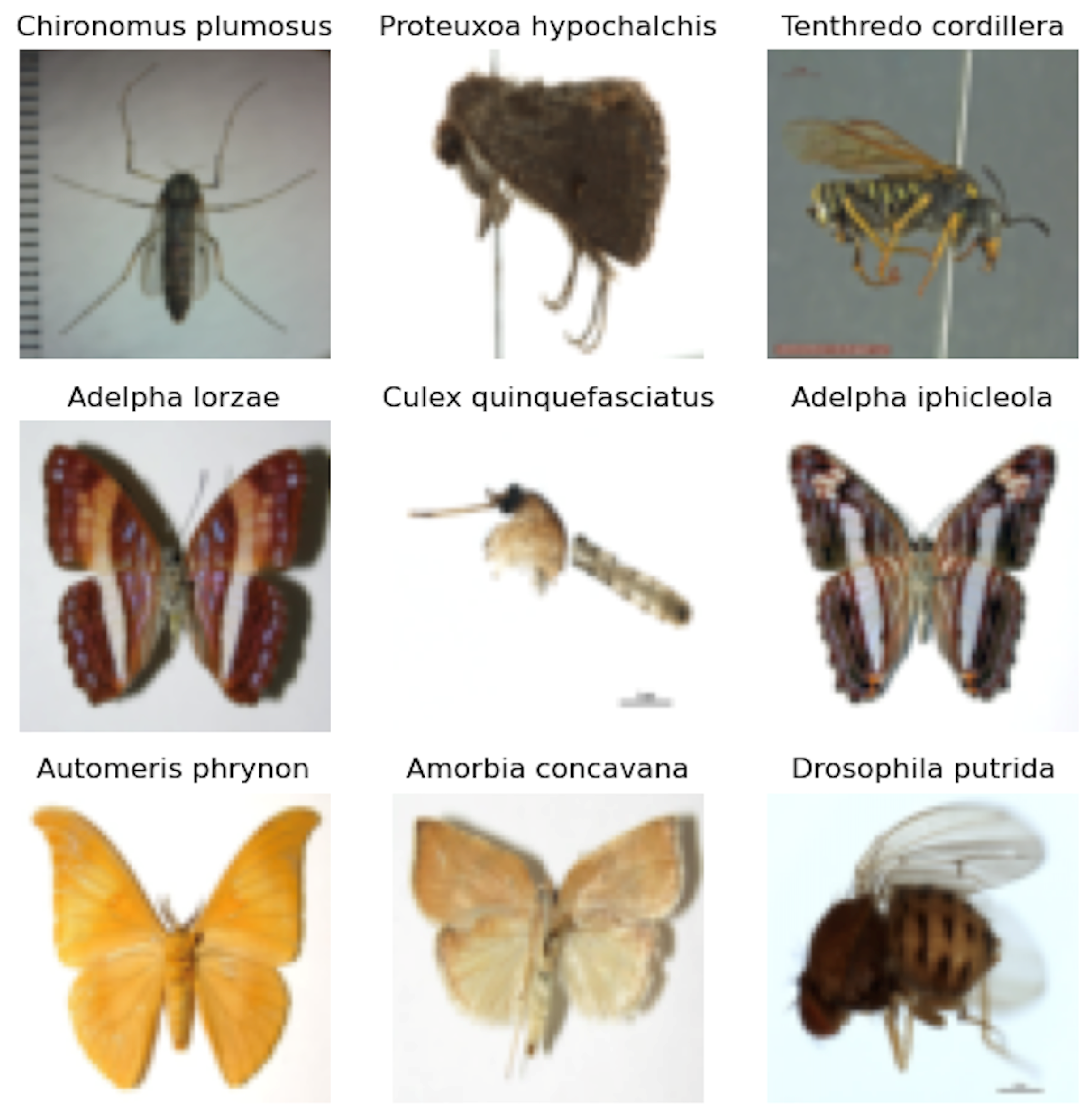
In accordance with the methodology outlined in the original paper, the data utilized in our experiments were obtained from the Barcode of Life Data System (BOLD) [6], which is a cloud-based data storage and analysis platform developed at the Centre for Biodiversity Genomics in Canada. The data consist of 32,424 image samples, e.g., see Figure 2, of insect species from four Insecta orders, Diptera, Coleoptera, Lepidoptera, and Hymenoptera, each associated with a DNA barcode COI mitochondrial sequence of that species.

Due to the fact that we did not have access to the original images used in [16], we resorted to downloading the data from the BOLD Systems platform to recreate a dataset that closely matches [16]. However, we encountered some discrepancies: some species names have been updated, and certain species have been split into two distinct categories. As a result, our dataset exhibits some differences compared to [16].

Table 1. Differences in the collected dataset compared to [16], the columns Genera and Species report the number of classes of the samples.

	Genera	Species	Samples
[16]	368	1040	32,848
Here	371	1050	32,424

highlights these differences.

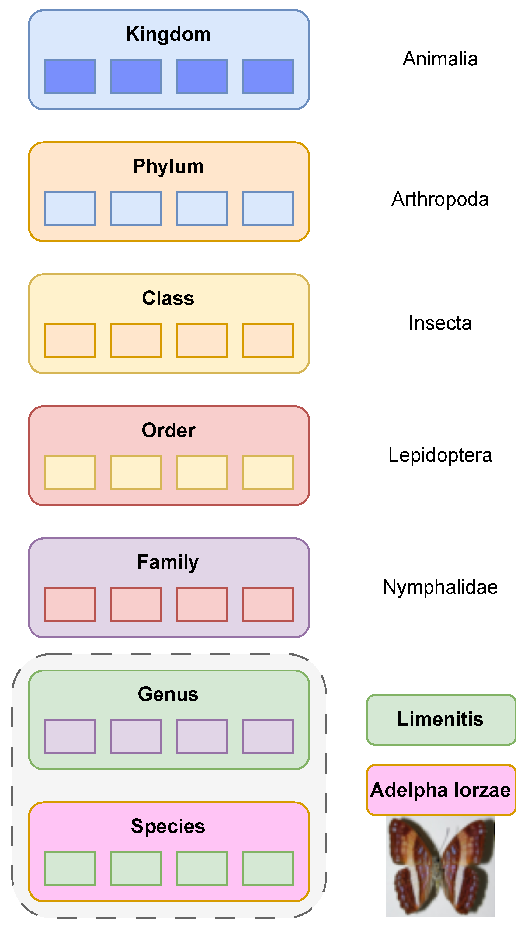
Next, we split the data following the methodology described in [16]. We considered all genera containing three or more species and we randomly selected 30% of the species within each of these genera as “undescribed” (only the genus is known while the species is unknown) and added all the samples from these species in the test set. We then split the remaining described data into 80% for the training + validation and 20% for the test set. Hence, the final test set consists of this 20% together with the previously designated undescribed species. This process is described by Algorithm 1. After applying Algorithm 1 to obtain a training + validation set and a test set, we apply it again on the training + validation set to obtain a training set with only described species and a validation set with both described and undescribed species. It is necessary that the undescribed species in the validation set are different species from the undescribed species in the test set; this is important to avoid class leaking from the test set to the validation set, ensuring that the undescribed species in the test set remain unseen during validation.

Algorithm 1 Split dataset to simulate undescribed species
Require: D       ▹ Dataset to split, containing species and their genus
Ensure: training, test         ▹ Split dataset with undescribed species
1:	Initialize $test\leftarrow \varnothing$
2:	Group species in D by genus
3:	for all genus g in D where $\left|g\right|\ge 3$ do
4:	Randomly select 30% of species in g as $undescribed$
5:	Add all samples in D with $undescribed$ species to $test\_unseen$
6:	Remove samples with $undescribed$ species from D
7:	end for
8:	Split the remaining D into $training$ (80%) and $test\_seen$ (20%)
9:	$test$ = $test\_seen$∪$test\_unseen$
10:	return $training$, $test$

We did not use the validation set for the training or the hyperparameter tuning of our models described in Section 3.4, but we provide this validation set to be used in future works that use the same dataset in order to be able to compare our results.

3.2. Dataset with Undescribed Species

To create a dataset of real-life undescribed species, we began by listing all genera present in the BOLD dataset containing simulated undescribed species. Using this list, we queried the BOLD Systems database to download samples belonging to these genera but with no species name, indicating that they were undescribed at the time of data retrieval. From these downloaded samples, we randomly selected 5% to ensure the dataset was comparable in size to the one containing simulated undescribed species. As a result, the final dataset contains 40,050 samples (image and COI mitochondrial DNA sequence) representing real-life undescribed species. This dataset is used entirely as a test set, while training is carried out using the dataset described in Section 3.1.

3.3. Beetle and Fish Datasets

Two other datasets with global coverage for specific groups have been used. Both of them, namely the Beetle and Fish datasets, have been proposed in [27], requiring a minimum of five images per species. The Beetle dataset comprises 615 mitochondrial COI fragments from 123 beetle species across three families: Coccinellidae, Cantharidae, and Anthribidae. The Fish dataset includes 1070 mitochondrial COI fragments representing 214 fish species from 15 families. These groups served as excellent test cases to evaluate the algorithm power and robustness; just to show the generalizability of the method, we also used a dataset of fishes that is not related to insects.

3.4. Feature Extraction

All the models presented in this section have been trained only on the training set of the dataset with simulated undescribed species presented in Section 3.1, without any hyperparameter tuning using the validation set. After the training, the weights of the models have been saved and used to extract the features from the other datasets.

We reproduced the methodology detailed in [16] using our data. To reproduce their DNA feature extraction technique, we used the same Convolutional Neural Network (CNN) architecture but we changed the activation function of the fully-connected layer from Tanh to LeakyReLU because we experienced vanishing gradient. For the image features, we used a pre-trained Resnet101 that gave us a vector of 2048 features. The Resnet was not fine-tuned, as described in [16].

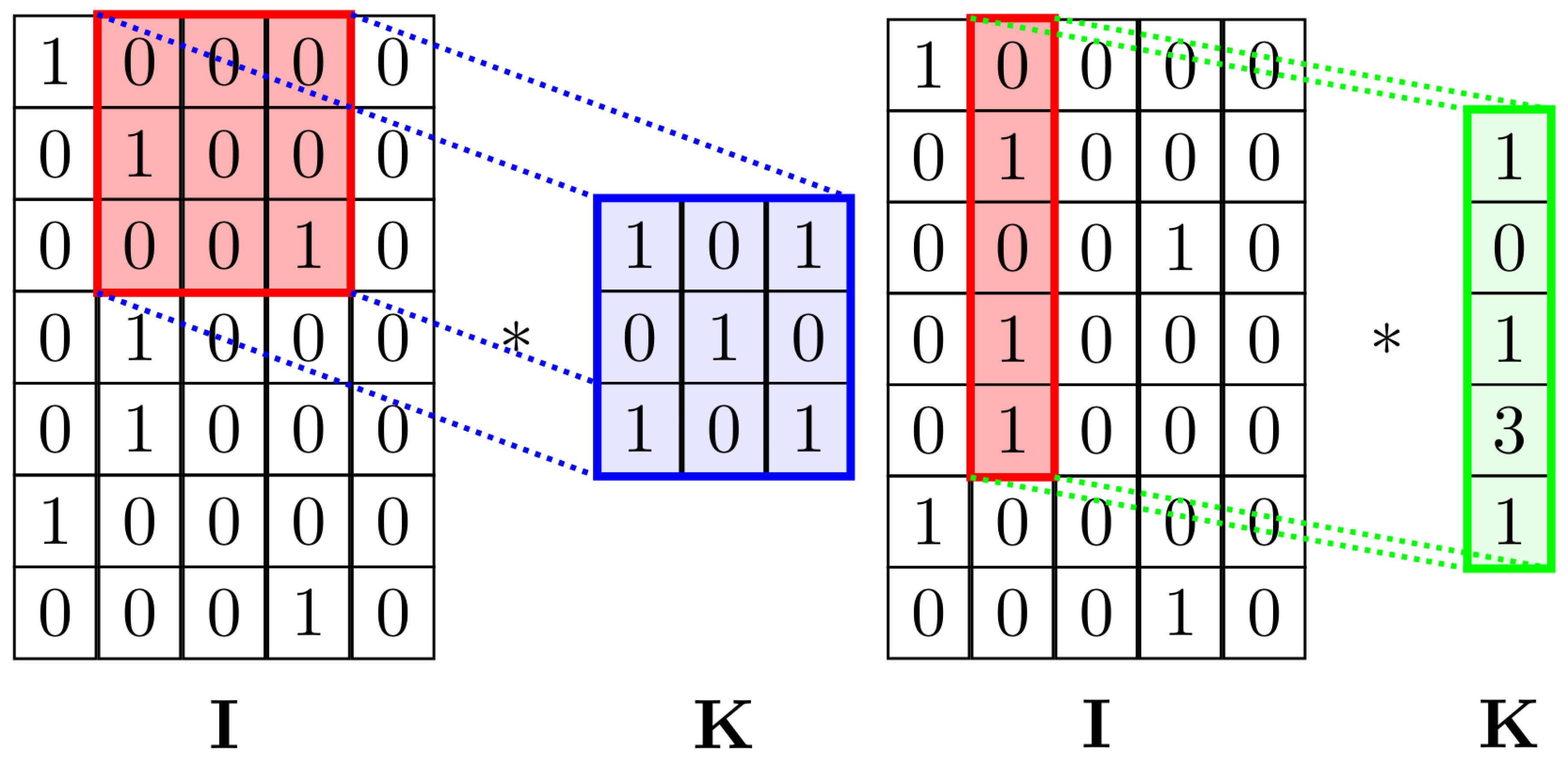
Our method also used a CNN to extract the DNA features. Our CNN architecture consists of 2 convolutional layers, both of which use a one-dimensional ($5\times 1$) kernel (in order to avoid reducing too much the output dimension), batch normalization, and LeakyReLU as the activation function. A dropout layer is used (70% dropout rate) after the second convolutional layer. The vectors are then flattened and projected on a linear layer of size 1500, followed by another dropout (70% dropout rate) and a LeakyReLU as mentioned before. The output is finally projected on a linear layer of size equal to the number of classes.

The main idea behind using the $5\times 1$ convolution instead of $3\times 3$ as in the original paper was to maintain the shape of the second dimension of the tensor constant without using padding. This allows the CNN to focus on finding local patterns in neighboring nucleotides (Figure 3). Using $3\times 3$ kernels would mean also considering convolutions across the one-hot encoding of a single nucleotide, possibly losing positional information and finding irrelevant relations.

Furthermore, for extracting the image features, we used the intermediate layer of the discriminator of a conditional Generative Adversarial Network (GAN) model, named Rebooted Auxiliary Classifier Generative Adversarial Network (ReACGAN). ReACGAN [35] is a newer version of the ACGAN model (a model of conditional GAN) with the purpose of improving the stability of the training by using residual connections (similar to ResNet), spectral normalization, embedding normalization, conditional batch normalization, and a different loss. ReACGAN aims to solve the exploding gradient and mode collapse problems that occur in ACGAN when the dataset contains a high number of classes. Since we were experiencing mode collapse with regular ACGANs due to having a large number of classes, we decided to use this improved version. The residual connections are the same as in ResNet.

Spectral normalization, introduced in [36] to stabilize the training of the discriminator, is applied to both the layers of the generator and the discriminator in the ReACGAN. It works on the weight matrix W applying (Equation (1)), where h is a randomly initialized vector. This is equivalent to dividing the matrix by its maximum singular value.

$$\underset{\mathbf{h}:\mathbf{h}\ne \mathbf{0}}{max}{\displaystyle \frac{{\parallel Wh\parallel }_2}{{\parallel h\parallel }_2}}$$

(1)

Conditional batch normalization (Equation (3)) differs from regular batch normalization (Equation (2)) by determining the values of the parameters $\beta$ and $\gamma$ using a linear layer from the input features instead of learning one value for them. In conditional GANs it allows the model to learn different scaling factors for different classes of samples (e.g., different species or genera).

$$\gamma \left({\displaystyle \frac{x-\mu }{\sigma }}\right)+\beta$$

(2)

$${\mathrm{MLP}}_{\gamma }\left(x\right)\left({\displaystyle \frac{x-\mu }{\sigma }}\right)+{\mathrm{MLP}}_{\beta }\left(x\right)$$

(3)

where $\mu$ and $\sigma$ are the mean and the standard deviation of the values of elements of the batch. It has been proved, by [35], that in ACGAN discriminators the gradients scale with the norm of the sample embedding (the feature extracted by the discriminator).

Finally, the D2D-CE (data-to-data cross-entropy) loss is used. Normally, ACGANs compute the cross-entropy between the feature extracted by the discriminator (called sample embedding) and the embedding of the class label which is called proxy (in ACGANs, a one-hot encoding of the label can be used instead of an embedding of the class label).

In [35] it is showed how normalizing the sample embedding and the label proxy avoids the exploding gradient problem that appears at early training and is one of the causes of early mode collapse.

Equations (4) and (5) describe the common cross-entropy and the D2D-CE loss functions, respectively. Both are expressed by considering $F\left(\mathbf{x}\right)$, the feature embedding vector extracted from image x by the penultimate layer of the discriminator, and $W=[{\mathbf{w}}_1,\cdots ,{\mathbf{w}}_c]$, which is the weight matrix of the last layer of the discriminator.

$${\mathcal{L}}_{\mathrm{CE}}=-{\displaystyle \frac{1}{N}}\sum _{i=1}^{N}log\left({\displaystyle \frac{exp\left(F{\left({\mathbf{x}}_i\right)}^{\top }{\mathbf{w}}_{y_i}\right)}{{\sum }_{j=1}^{c}exp\left(F{\left({\mathbf{x}}_i\right)}^{\top }{\mathbf{w}}_j\right)}}\right).$$

(4)

$${\mathcal{L}}_{\mathrm{D}2\mathrm{D}-\mathrm{CE}}=-{\displaystyle \frac{1}{N}}\sum _{i=1}^{N}log\left({\displaystyle \frac{exp({[{\mathbf{f}}_i^{\top }{\mathbf{v}}_{y_i}-m_p]}_{-}/\tau )}{exp({[{\mathbf{f}}_i^{\top }{\mathbf{v}}_{y_i}-m_p]}_{-}/\tau )+{\sum }_{j\in \mathcal{N}\left(i\right)}exp\left({[{\mathbf{f}}_i^{\top }{\mathbf{f}}_j-m_n]}_{+}/\tau \right)}}\right),$$

(5)

The D2D-CE (Equation (5)) is a modified version of CE (Equation (4)), where ${\mathbf{v}}_{y_i}={\displaystyle \frac{{\mathbf{w}}_{y_i}}{\left|\right|{\mathbf{w}}_{y_i}\left|\right|}}$ and ${\mathbf{f}}_i={\displaystyle \frac{P\left(F\left({\mathbf{x}}_i\right)\right)}{\left|\right|P\left(F\left({\mathbf{x}}_i\right)\right)\left|\right|}}$, P is a projection carried out by a linear layer, ${[·]}_{-}$ = min(·,0) ${[·]}_{+}$ = max(·,0), $\mathcal{N}\left(i\right)$ is the set of indices of the samples in the minibatch for which the label is different from $y_i$ (it is the real label); the margins $m_p$ and $m_n$ and the temperature $\tau$ are hyperparameters, and we use the implementation and the values of the hyperparameters suggested in [37].

Also in D2D-CE, the denominator (Equation (5)) of the softmax still computes the similarity between the sample embedding and the proxy (either one-hot or embedding) in order to consider data-to-class similarities, but in the denominator, we split the summation in two: a term equal to the numerator plus a term that computes the similarities between the sample embeddings for images of the batch belonging to different classes ($j\in \mathcal{N}\left(i\right)$). This second term does not consider data-to-class relationships because it does not involve the weights of the last layer ${\mathbf{v}}_{y_i}$. Conversely, it considers relationships between the sample embeddings of different classes. For this reason, the loss function is called Data-to-Data CE.

This makes it so that by minimizing the loss, we make the sample embeddings more similar to the corresponding class proxies, but at the same time, we make the sample embeddings of images belonging to different classes different between each other. This idea is similar to the contrastive loss used in siamese networks.

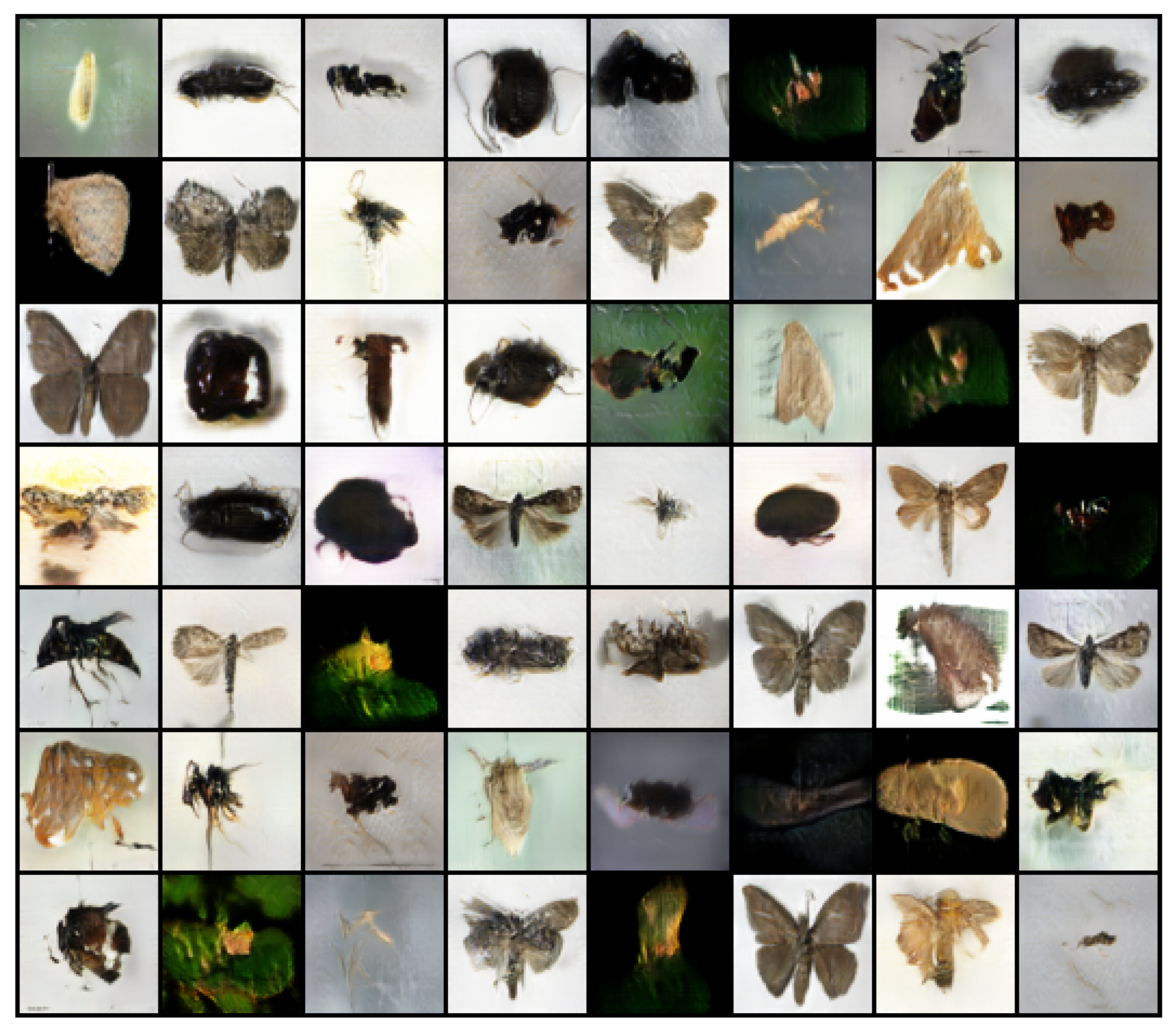
The intuition behind this loss is that we make the discriminator use visual features from the images to distinguish images of different classes instead of just making it only guess the class directly. If this intuition is correct, it would be useful for our purpose since our objective is not just to generate realistic images but to also obtain useful features that encode the class of the insect. Some sample obtained by ReACGAN are shown in Figure 4.

The last step to obtain the final version of D2DCE (Equation (5)) is to consider the 3 hyperparameters: the margins $m_p$ and $m_n$ and the temperature $\tau$. Since the model is too big for our dataset, we pre-trained it on a dataset of arbitrary animals taken from various internet datasets for 25 epochs. Then, we fine-tuned it on our dataset for 12 epochs.

The dataset for the pre-training of the ReACGAN contains [38] and some other datasets from kaggle with pictures of insects and other animals. The whole pre-training dataset can be found at [39].

3.5. Discrete Wavelet Transform

In numerical analysis and functional analysis, a discrete wavelet transform (DWT) is a type of wavelet transform where the wavelets are discretely sampled. A significant advantage of DWT compared to Fourier transforms is its ability to provide temporal resolution, capturing both frequency and time location information [40].

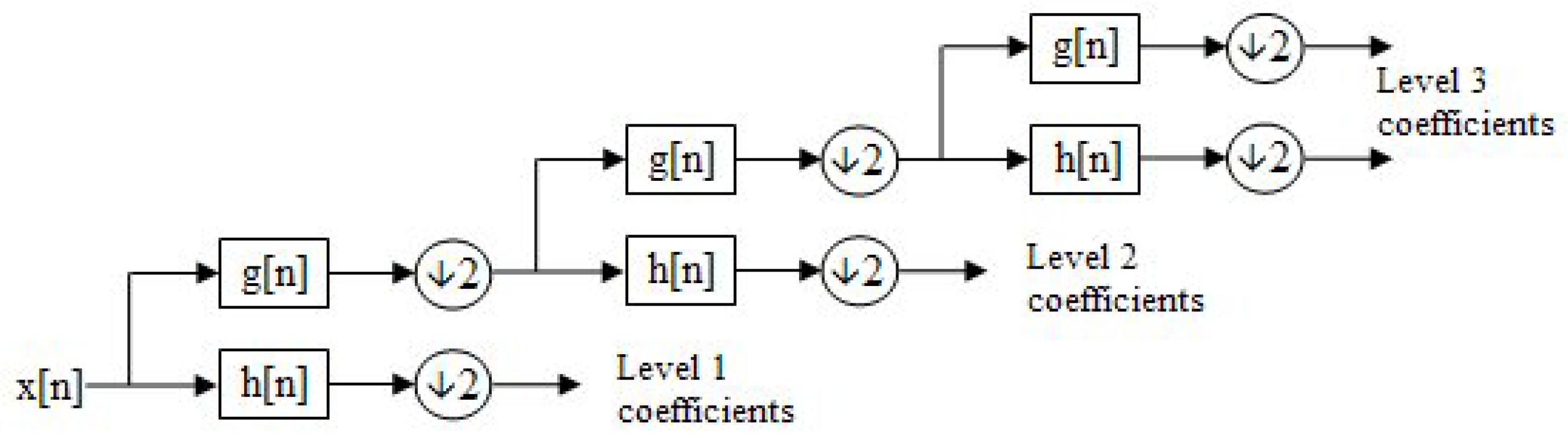
Given a 1D discrete signal $x\left[n\right]$, the DWT is calculated by passing the signal through two filters:

• A low-pass filter $h\left[n\right]$ (scaling function);
• A high-pass filter $g\left[n\right]$ (wavelet function).

The outputs of these filters are downsampled by a factor of 2 to reduce the number of coefficients, effectively halving the time resolution. The signal decomposition can be expressed as follows: 

$$cA\left[n\right]=\sum _{k}x\left[k\right]h[n-k]$$

$$cD\left[n\right]=\sum _{k}x\left[k\right]g[n-k]$$

where $cA\left[n\right]$ comprises the approximation coefficients (low-frequency components) and $cD\left[n\right]$ comprises the detail coefficients (high-frequency components).

The filtering and downsampling process is recursive. After each decomposition, the approximation coefficients are further decomposed into new approximation and detail coefficients at the next level.

This decomposition process is visualized as a binary tree, see Figure 5, where each node represents a sub-space with distinct time-frequency localization. This structure is commonly referred to as a filter bank.

The proposed approach utilizes the following mother wavelets:

• Haar;
• Daubechies;
• Symlets;
• Coiflets;
• Biorthogonal;
• Reverse Biorthogonal;
• Discrete Meyer;
• Fejér–Korovkin Orthogonal;
• Beylkin Orthogonal;
• Vaidyanathan Orthogonal.

We did not perform a study to overfit which wavelets to use, instead using the ones available in MATLAB and using the default parameters; the same set is used for all the datasets, so we assume that there is no risk of overfitting. Below is the pseudocode for the described approach; see pseudocode Algorithm 2. This process is applied three times to create the 3 channels of the matrix used for feeding ResNet50.

Algorithm 2 DWT approach for reshaping data

Ensure: Define $vector$ the feature vector that describes a given pattern Initialize a square matrix Mat of size $\lceil {\displaystyle \frac{\mathrm{length}\left(vector\right)}{8}}\rceil$ filled with zeros. Define $num\_levels={log}_2\left(\mathrm{length}\left(vector\right)\right)$ $row\leftarrow 1$ $OrigVector$ = $vector$;                  ▹ Original feature vector for $diffWavelet$ = 1:inf do             ▹ Iterate over wavelet types;     $vector$ = $OrigVector$;        ▹ Fill the matrix Mat with wavelet coefficients     for $filter$ = 1:($num\_levels$ - 4) do▹ Discard the last 4 levels due to low dimensionality         [$approximation$, $detail$] = apply wavelet to ‘vector’; ▹ Randomly choose mother wavelet for this iteration, extract approximation and detail coefficients. Such choice is random for each network, obviously for each pattern in a given network the same set of mother wavelets is used.         $vector$ = $approximation$;      ▹ Use approximation vector for next iteration         - Check(filter==1, $approximation$, $detail$) At the first filter bank level, approximation and detail coefficients are resized to 25% of their size.         - Check(filter==2, $approximation$, $detail$) At the second filter bank level, coefficients are resized to 50%.      ▹ the rationale is to avoid reducing the dimensionality of the other levels, important to underline that the output matrix will be resized to the size required by ResNet50 (i.e., square matrix of size 224 with 3 channels)         Mat(row, :) = $approximation$;         Mat(row+1, :) = $detail$;         row = row + 2;     end for     if $row$ > size(Mat, 2) then▹ Exit condition: if row is higher than the number of rows of Mat         break;     end if end for

3.6. Classification Approaches: Support Vector Machine and ResNet50

One of the most influential approaches to supervised learning is the support vector machine [41]. This method is parameterized by a set of N weights $\mathbf{w}\in {\mathbb{R}}^N$ and a bias term $b\in \mathbb{R}$. In a binary classification task, the SVM predicts a class $y\in \{-1,1\}$ for a sample vector $\mathbf{x}\in {\mathbb{R}}^N$ using the following decision function:

$$y=sgn\left({\mathbf{w}}^{\top }\mathbf{x}+b\right),$$

(6)

which defines a hyperplane in ${\mathbb{R}}^N$ referred to as margin. The margin, or the distance between the hyperplane and the closest points from each class, is maximized during training to achieve optimal separation. For multi-class classification, the problem becomes more complex and can be approached in various ways. A common method is the one-vs-one strategy, which divides the task into multiple binary classification problems, one for each pair of classes. The final prediction is computed by majority voting, often incorporating distance from the margin as a tiebreaker. However, this approach requires training an SVM for every class pair, which can significantly increase computational costs. Another strategy is the one-vs-all, which requires to train a model for each unique class in order to distinguish it from all the other classes. The final prediction is computed by selecting the class for which the model predicts the highest margin. Compared to the one-vs-one strategy, the one-vs-all is more robust to an imbalanced dataset and is particularly fast to train, especially when the number of classes is large. Here, we used the one-vs-all approach and the LibSVM toolbox (https://www.csie.ntu.edu.tw/~cjlin/libsvm/, accessed on 8 February 2025).

ResNet (Residual Network), introduced by Hen [42], is a deep learning architecture designed to address the vanishing gradient problem in training deep neural networks. It introduces residual connections, or skip connections, that allow gradients to flow directly through the network, bypassing one or more layers. This is achieved by reformulating the layers to learn a residual mapping $F\left(\mathbf{x}\right)=H\left(\mathbf{x}\right)-\mathbf{x}$, where $H\left(\mathbf{x}\right)$ is the original mapping, and the output is $F\left(\mathbf{x}\right)+\mathbf{x}$. ResNet is highly effective for multi-class classification tasks. The network consists of stacked residual blocks, each comprising convolutional layers, batch normalization, and ReLU activations, with a skip connection that adds the input of the block to its output. The architecture scales to hundreds or thousands of layers while maintaining high performance. ResNet models are often initialized with weights pre-trained on the dataset ImageNet [43], leveraging features learned from over a million diverse images, a technique also known as transfer learning. This approach accelerates convergence, improves performance on downstream tasks, and is computationally efficient compared to training a deep network from scratch. Each net is trained for 10 epochs, with a batch size equal to 30, a learning rate 0.001, and stochastic gradient descent (SGD) for optimization.

4. Results

In this section, the different approaches are compared using the five datasets described in Section 3. The classification performance for the Badirli dataset (performance is reported in Table 2) and the two datasets proposed here, see Section 3.1 (performance is reported in Table 3) and Section 3.2 (performance is reported in Table 4), was assessed by the weighted species accuracy and the weighted genus accuracy:

$$\mathrm{Weighted}\mathrm{Accuracy}={\displaystyle \frac{1}{n}}\sum _{j=1}^n{\displaystyle \frac{y_j}{n_j}},$$

(7)

where for class j, $y_j$ is the number of correctly classified patterns of class j, $n_j$ is the total number of patterns for that class, and n is the number of species or the number of genera. Notice that this is the same formula for the weighted species accuracy and the weighted genus accuracy.

Instead, for the Beetle and Fish datasets, the standard accuracy is used as a performance indicator, as in the related literature; the performance is reported in Table 5 and Table 6.

The following methods are reported in this section:

• Bad, the method detailed in [16];
• Bad_D, the method, based only on DNA barcoding, detailed in [16];
• SVM_D, SVM trained using the features proposed in [16] to represent the DNA sequence;
• SVM_O, SVM trained using the features proposed in [16] to represent both the DNA sequence and image;
• SVM_N, SVM trained using the features proposed in this paper to represent both DNA sequence and image;
• SVM_f, sum rule between SVM_O and SVM_N;
• DWT_O, an ensemble of 15 ResNet50 trained using the DWT approach coupled with the features proposed in [16] to represent both the DNA sequence and image;
• DWT_N, an ensemble of 15 ResNet50 trained using the DWT approach coupled with the features proposed in this paper to represent both the DNA sequence and image;
• DWT_f, sum rule between DWT_O and DWT_N;
• DWT_O + SVM_O, sum rule between DWT_O and SVM_O;
• DWT_f + SVM_f, sum rule between DWT_f and SVM_f;
• eDNA, the method proposed in [44] for DNA barcoding classification;
• Proposed, the weighted sum rule among $0.5\times {\mathrm{DWT}}_f+1\times {\mathrm{SVM}}_f+1\times \mathrm{eDNA}$.

Not all methods are reported for all datasets; for example, in the case of the Badirli dataset, since we do not have any images available, we cannot calculate the new features detailed in Section 3.4. In both the Fish and Beetle datasets, the performance of SVM with original features is low; to reduce computation time, we did not compute DWT_O and, therefore, the method named “Proposed” for the Beetle and Fish dataset is given by the following: $0.5\times {\mathrm{DWT}}_N+1\times {\mathrm{SVM}}_N+1\times \mathrm{eDNA}$.

Notice that, before the sum rule, the scores of each approach are normalized to mean 0 and standard deviation 1.

In the tests reported in the following Table 2 and Table 3, we suppose that an oracle divides the animals between those with known species and those only with known genera. In the final test, reported in Figure 6, we adopt a robust protocol in which all animals are classified at the species level, using a rejection threshold; those not classified in any species are classified at the genus level: this test is similar to a real application of this kind of problem.

While accuracy provides an overall measure of the model’s performance, it does not fully capture the nuances of classification performance, especially for imbalanced datasets. Therefore, we will extend the evaluation metrics to include Precision and Recall for comparing our proposed ensemble with the baseline SVM. Precision (PR) and Recall (RE) are defined as follows:

$$Precision={\displaystyle \frac{TP}{TP+FP}}$$

(8)

$$Recall={\displaystyle \frac{TP}{TP+FN}}$$

(9)

where $TP$ = true positives; $FP$ = false positives; and $FN$ = false negatives. In Table 7, we report PR and RE for comparing our proposed ensemble with SVM_f, when it is available, or SMV_O. This test provides further confirmation of the effectiveness of the proposed ensemble compared to the SVM ensemble. This is significant, as SVM remains one of the most widely used classifiers in both the academic literature and practical applications.

Table 2. Accuracy of different methods on the Badirli Dataset.

Badirli	Species	Genus
Bad	98.21	81.95
BadD	98.65	71.85
[45]	99.47	83.22
SVMD	99.20	80.23
SVMO	99.22	81.26
DWTO	99.17	76.57
DWTO + SVMO	99.40	81.92
eDNA	98.74	87.20
Proposed	99.47	87.74

Table 2. Accuracy of different methods on the Badirli Dataset.

Badirli	Species	Genus
Bad	98.21	81.95
BadD	98.65	71.85
[45]	99.47	83.22
SVMD	99.20	80.23
SVMO	99.22	81.26
DWTO	99.17	76.57
DWTO + SVMO	99.40	81.92
eDNA	98.74	87.20
Proposed	99.47	87.74

Table 3. Accuracy of different methods on the New Insects Dataset, Section 3.1.

New Insects	Species	Genus
[45]	99.05	84.02
SVMD	99.16	79.07
SVMO	98.21	82.01
SVMN	98.05	65.05
SVMf	99.00	83.67
DWTO	98.83	75.08
DWTN	98.54	82.98
DWTf	99.12	83.85
DWTf + SVMf	99.15	85.51
eDNA	98.48	88.49
Proposed	98.99	91.35

Table 3. Accuracy of different methods on the New Insects Dataset, Section 3.1.

New Insects	Species	Genus
[45]	99.05	84.02
SVMD	99.16	79.07
SVMO	98.21	82.01
SVMN	98.05	65.05
SVMf	99.00	83.67
DWTO	98.83	75.08
DWTN	98.54	82.98
DWTf	99.12	83.85
DWTf + SVMf	99.15	85.51
eDNA	98.48	88.49
Proposed	98.99	91.35

Table 4. Accuracy of different methods on the Unseen Dataset, Section 3.2.

Unseen	Genus
SVMD	23.85
SVMO	32.75
SVMM	46.82
SVMf	47.70
DWTO	30.38
DWTN	28.25
DWTf	42.73
DWTf + SVMf	48.15
eDNA	33.36
Proposed	48.56

Table 4. Accuracy of different methods on the Unseen Dataset, Section 3.2.

Unseen	Genus
SVMD	23.85
SVMO	32.75
SVMM	46.82
SVMf	47.70
DWTO	30.38
DWTN	28.25
DWTf	42.73
DWTf + SVMf	48.15
eDNA	33.36
Proposed	48.56

Table 5. Accuracy of different methods on the Beetle Dataset.

Beetle	Species
[27]	98.10
[45]	98.20
SVMD	95.13
SVMO	90.48
SVMN	97.69
SVMf	97.69
DWTO	—
DWTN	62.72
DWTr	86.66
DWTr + SVMf	98.03
eDNA	98.20
Proposed	98.51

Table 5. Accuracy of different methods on the Beetle Dataset.

Beetle	Species
[27]	98.10
[45]	98.20
SVMD	95.13
SVMO	90.48
SVMN	97.69
SVMf	97.69
DWTO	—
DWTN	62.72
DWTr	86.66
DWTr + SVMf	98.03
eDNA	98.20
Proposed	98.51

Table 6. Accuracy of different methods on the Fish Dataset.

Fish	Species
[27]	96.30
SVMD	94.75
SVMO	91.73
SVMN	95.70
SVMf	95.61
DWTO	—
DWTN	93.22
DWTr	92.82
DWTr + SVMf	96.83
eDNA	96.75
Proposed	97.03

Table 6. Accuracy of different methods on the Fish Dataset.

Fish	Species
[27]	96.30
SVMD	94.75
SVMO	91.73
SVMN	95.70
SVMf	95.61
DWTO	—
DWTN	93.22
DWTr	92.82
DWTr + SVMf	96.83
eDNA	96.75
Proposed	97.03

Table 7. Precision–Recall performance indicator on different datasets.

Dataset	Approach	Precision	Recall
Beetle	SVMf	99.73	100
	Proposed	99.81	100
Fish	SVMf	99.48	100
	Proposed	99.57	100
Badirli—Species	SVMO	99.82	98.71
	Proposed	99.42	99.14
Badirli—Genus	SVMO	90.16	85.74
	Proposed	93.17	92.02
New—Species	SVMf	99.46	99.00
	Proposed	99.38	98.99
New—Genus	SVMf	90.91	89.69
	Proposed	95.90	95.63
Unseen	SVMf	57.29	53.91
	Proposed	58.11	54.50

Table 7. Precision–Recall performance indicator on different datasets.

Dataset	Approach	Precision	Recall
Beetle	SVMf	99.73	100
	Proposed	99.81	100
Fish	SVMf	99.48	100
	Proposed	99.57	100
Badirli—Species	SVMO	99.82	98.71
	Proposed	99.42	99.14
Badirli—Genus	SVMO	90.16	85.74
	Proposed	93.17	92.02
New—Species	SVMf	99.46	99.00
	Proposed	99.38	98.99
New—Genus	SVMf	90.91	89.69
	Proposed	95.90	95.63
Unseen	SVMf	57.29	53.91
	Proposed	58.11	54.50

The following conclusions can be obtained considering the tables reported in this section:

• In each dataset, one of the methods tested in this paper gets the new SOTA, and ensemble is proposed as the best method among the tested approaches. In general, the conclusions are different whether we use the large datasets or the two small ones (i.e., Beetle and Fish); this is, logically, because of the size of the training set, a more important factor for neural networks than SVM.
• Interestingly, between SVM and DWT, there is no winner; in some cases, SVM does better, in others DWT. However, their fusion allows both methods to improve. Performance is similar in the three large datasets, while in Beetle and Fish, which are much smaller in size, SVM performs much better than DWT; it is assumed that this is due to the fact that DWT is based on neural networks, which require a larger training set size than SVM.
• Similarly, also between the features proposed in [16] and those proposed in this paper, there is no clear winner; however, the fusion allows to improve the results of the individual methods. Again, there is a difference in the results between the three large datasets and the two smaller ones (Beetle and Fish), in which the features proposed in [16] perform badly.

In the final test, reported in Figure 6, we adopt a realistic protocol for the proposed dataset, i.e., the one detailed in Section 3.1, where all the insects are first classified at the species level (the species are the classes); notice that we have two trained nets, one for species and one for genera classification. Let us suppose the following:

• ${\theta }_1\left(\mathbf{x}\right)$ is the highest score (obtained using the species classification net) among the different species (i.e., classes) given a pattern x;
• ${\theta }_2\left(\mathbf{x}\right)$ is the second highest score (obtained using the species classification net) of that pattern;
• $\theta \left(\mathbf{x}\right)={\theta }_1\left(\mathbf{x}\right)-{\theta }_2\left(\mathbf{x}\right)$.

Our rejection criteria are as follows:

• If $\theta \left(\mathbf{x}\right)>\tau$, the insect is assigned to a species class; otherwise, it is assigned to a genus class (i.e., it is classified by the network trained using the genus as classes).
• If a pattern belongs to a known species but is classified at the genus level, it is considered a classification error; clearly, a pattern with an unknown species is regarded as an error if classified at the species level.

In Figure 6, we report the plot of the species accuracy (x-axis) versus genus accuracy (y-axis) obtained by varying the rejection threshold $\tau$. The green line is obtained by SVM_f, and the black line by our ensemble ‘Proposed’. This test clearly shows the usefulness of the proposed ensemble versus SVM.

5. Discussion

Several interesting insights can be drawn from the results presented in the previous section. Let us examine some of them.

• As is often the case in machine learning and deep Llearning, no single method consistently outperforms all others across the datasets tested in this study. Instead, the best results are achieved through an ensemble approach. This suggests that different methods capture distinct aspects of the data, and their combination allows for a more comprehensive extraction of information, ultimately leading to superior performance compared to individual methods.
• It is important to highlight that methods relying solely on image-based features perform worse than those based on DNA barcoding. However, integrating both types of features—those extracted from images and those derived from DNA information—enhances the performance of a DNA-only classifier.
• Even when compared to state-of-the-art methods across various datasets, our ensemble approach emerges as the top performer. This reinforces our confidence that, despite the complexity of combining different techniques, the proposed ensemble method is robust across diverse datasets. As a result, it serves as a strong baseline for other researchers working with combined image and DNA barcoding data.
• Another notable observation comes from the plot in Figure 6. The proposed method demonstrates a substantial improvement over SVM, which is currently the most widely used classification technique; this highlights the potential usefulness of our system for the research community. Our method achieves impressive performance reaching 90% species-level accuracy and 90% genus-level accuracy; this is significantly higher than the results obtained with SVM. Moreover, these improvements have practical implications for expert naturalists, as they facilitate the identification of previously unknown species based on DNA barcoding and imaging with high accuracy.
• Finally, an interesting result reported in Table 4 pertains to the Unseen dataset, where species identities are unknown. Notably, DNA barcoding performs the worst in this dataset compared to the others tested. Nevertheless, even in this case, the ensemble method yields the best results. The fact that DNA barcoding does not significantly outperform image-based methods suggests that this dataset differs from the others. This further underscores the generalizability of the proposed approach.

As previously depicted, the results clearly show the usefulness of the ensemble proposed in this work; obviously, the disadvantage of the ensemble is the higher computational power required to perform inference and training. So, these ensemble-based methods are certainly not suitable for real-time analysis on edge computing devices, and they require the ability to access a server where modern GPUs are available. This is not a problem in many applications, e.g., thanks to low-cost satellite connections such as Starlink, it is relatively easy to have access to the network, so the number of projects in which an ensemble can be used has been increasing in recent years. In contrast, in all those applications where classification must be carried out on an unconnected device, simply because of the need to reduce power consumption, these approaches are not the ideal choice, because of the computing power required.

The experiments were conducted on the following hardware setup:

• Processor: Intel Core i5-12400 CPU (2.5 GHz, six cores);
• GPU: NVIDIA RTX 4070 (12 GB GDDR6X) for accelerated deep learning tasks;
• RAM: 32 GB DDR5;
• Programming Languages: Python 3.12.1 (for feature extraction tasks) and MATLAB 2024b (for wavelet transforms and classification). Deep Learning Framework: PyTorch 2.0, utilized for implementing and training the convolutional neural networks used for extracting features. LibSVM was used for support vector machines. MATLAB’s wavelet toolbox and deep learning toolbox were used to transform the feature vector into two-dimensional matrices and then to classify these using CNN.

The computation times achieved in our experiments are notably low, demonstrating the efficiency of the processes involved. Using a batch of 1000 patterns, the mean inference time for DNA barcoding feature extraction was only 0.256 s, reflecting swift performance even with complex biological data. Furthermore, the image feature extraction process exhibited exceptional speed, with a mean inference time of just 0.006 s. These results underline the computational efficiency of both methods, ensuring rapid data processing and scalability for larger datasets.

6. Conclusions

In this study, we investigated the performance benefits of combining neural networks with support vector machines (SVM). Our research contributes to the field by evaluating the effectiveness of integrating multiple classifiers to construct heterogeneous ensembles.

The key innovations introduced in this work are as follows. We proposed a novel method for building CNN ensembles by leveraging different mother wavelets for vector-to-matrix transformations and new methods for representing DNA sequences and images as feature vectors. We demonstrated the superior performance of the proposed method by comparing the ensembles with SVM-based models. We developed an ensemble that surpasses previous state-of-the-art approaches and standalone SVM models. For future work, we plan to extend our analysis by incorporating additional datasets to improve the generalization of our method. We also aim to explore alternative techniques from the literature for generating matrices suitable for CNN training. Further directions include devising new methods to describe DNA barcodes, incorporating images of individual insects, and developing approaches to reject patterns lacking species labels. Finally, we intend to focus on distillation techniques and continuous learning strategies to enable edge computing and the inclusion of numerous new classes, addressing the challenge of catastrophic forgetting.