Impact of Image Enhancement Using Contrast-Limited Adaptive Histogram Equalization (CLAHE), Anisotropic Diffusion, and Histogram Equalization on Spine X-Ray Segmentation with U-Net, Mask R-CNN, and Transfer Learning

Abstract

Image segmentation is one of the important applications of deep learning models, such as U-Net and Mask R-CNN, in medical imaging. The image segmentation process enables automated extraction of important information within images, including spine X-rays, saving medical practitioners hours of work. However, for X-ray images, low contrast and noise may affect the quality of the images and consequently reduce the effectiveness of the deep learning models in providing a robust segmentation. Image enhancement prior to feeding the images to segmentation models can help to overcome the issues caused by the low-quality images. This paper aims to evaluate the effects of three image enhancement methods, namely, the contrast-limited adaptive histogram equalization (CLAHE), histogram equalization (HE), and anisotropic diffusion (AD), for improving image segmentation performance of Mask R-CNN, non-transfer learning Mask R-CNN, and U-Net. The findings show image enhancement methods provide significant improvement to the U-Net, and, interestingly, no noticeable improvement of performance on Mask R-CNN is observed. The application of HE for transfer learning Mask R-CNN achieved the highest Dice score of 0.942 ± 0.001 for binary segmentation. The randomly initialized Mask R-CNN obtains the highest DSC of 0.941 ± 0.002 on the same task. On the other hand, for U-Net, despite the presence of statistically significant change by applying image enhancement methods, the model achieves a maximum Dice score of 0.916 ± 0.003, lower than Mask R-CNN with and without transfer learning. A study on image enhancement methods and recent deep learning algorithms is necessary to better understand the effect of image enhancement techniques using deep learning.

1. Introduction

Deep learning applications in the field of medical imaging analysis have seen a surge lately, spanning multiple clinical domains. Deep learning models like convolutional neural networks and transformers are applied for a variety of tasks related to medical imaging, including X-ray, CT-scan, and MRI images. Deep learning has also been applied to analyze the spine by providing diagnostic predictions of spine abnormalities [1], identifying spine segments and labeling [2], and also in providing a diagnosis for spine-related injuries [3].

The spine or vertebral column consists of 24 individual segments of vertebrae, not including 5 fused sacral vertebrae and 4 fused or separated coccyx. The individual segments of vertebrae include three regions: cervical with 7 segments, thoracic with 12 segments, and lumbar vertebrae with 5 segments. The spine provides structural support to the body, which is necessary for posture, balance, and gait [4,5]. Spine analysis may require the identification and segmentation of each vertebra.

Segmentation is a computer vision task focusing on dividing images into meaningful regions by providing each pixel in the image with a label. Deep learning models are commonly used for segmentation tasks of medical images and have demonstrated strong performance in identifying tumors [6], brain lesion detection [7], multi-organ segmentation [8], and musculoskeletal system analysis [9,10].

Spine images are commonly found in the form of X-ray images. X-ray is a type of medical imaging technique that utilizes electromagnetic radiation to penetrate the body and is recorded on either digital medium or physical film to produce images that consist of anatomical details of the body [11]. As reported by Mettler et al. [12], the effective X-ray radiation dose to visualize different body parts is different. X-ray was discovered in 1895, but remains a major medical imaging technique due to its lower cost and accessibility.

However, X-ray images are commonly affected by noise, which reduces the overall quality. The sources of X-ray noise are grain noise, electronic noise, structure noise, anatomical noise, and quantum noise [13]. Quantum noise is visible in the X-ray images when a low radiation dose is used. Electronic noise comes from the electronic signal generated by the power supply and within the electrical circuitry. Each of the noises can contribute to a lower quality of X-ray images, which may reduce the visibility of spine images used for medical procedures such as abnormality detection and injury assessment.

Contrast is an important factor influencing medical image analysis. It is described as the ratio of the signal difference relative to the average signal [14]. In medical images, a high contrast is desired, as a higher contrast enables images to be visualized better [14]. Typically, original medical images have pixel depths ranging from 10 to 14 bits. However, normal displays usually only output a grayscale pixel depth of 8 to 10 bits. This requires the usage of a window/level to convert the value from the original grayscale to the range of normal display [13]. This process may reduce the contrast visibility in the images. An observer’s ability to detect an object within an X-ray image is dependent on the noise and contrast of the object [14].

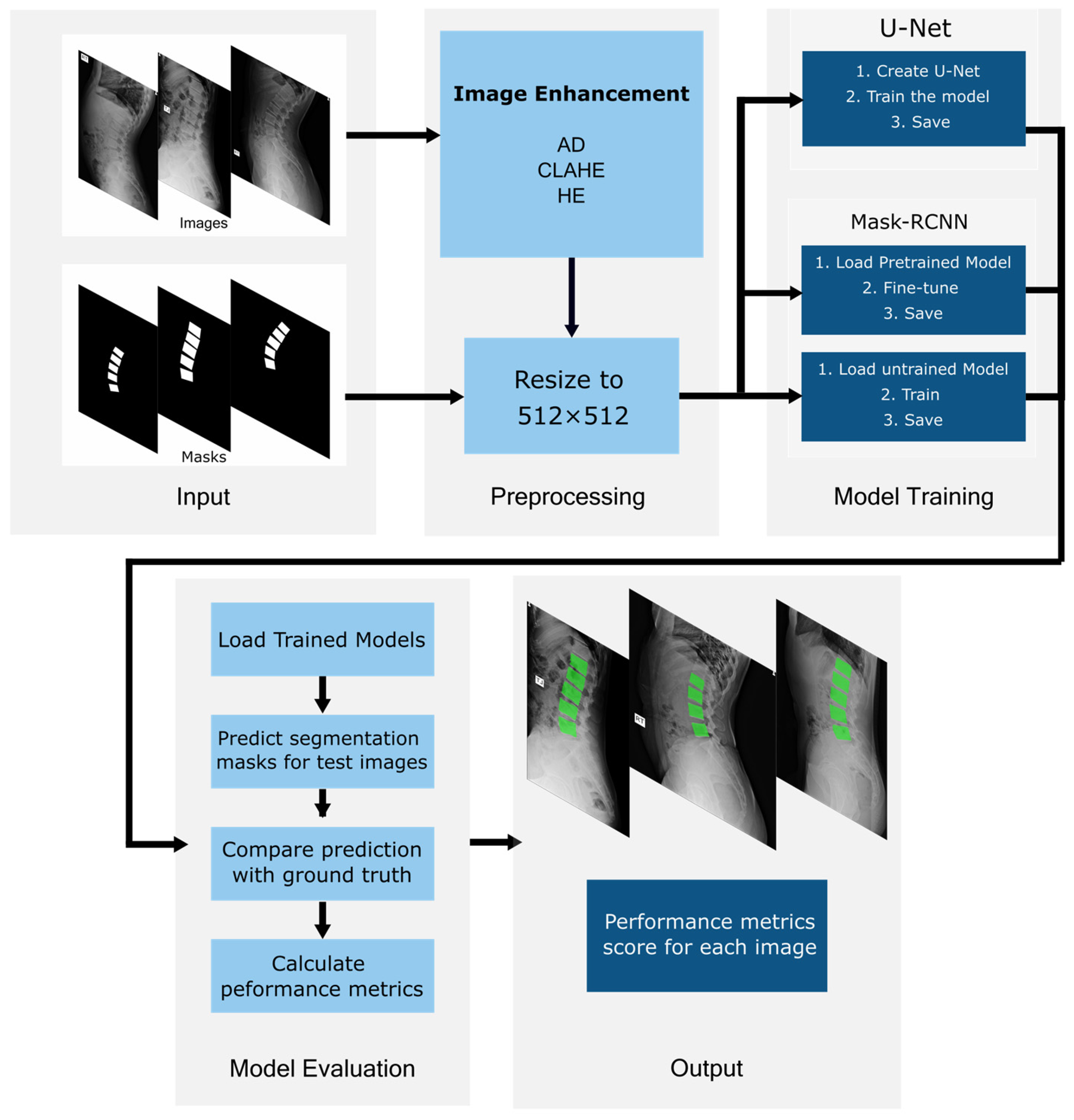
Despite extensive use of deep learning in medical imaging, the impact of image enhancement methods on X-ray segmentation performance remains underexplored. This study aims to systematically evaluate three widely used image enhancement techniques, specifically, the histogram equalization (HE), contrast-limited adaptive histogram equalization (CLAHE), and noise removal anisotropic diffusion (AD), and assess their influence on lumbar vertebrae segmentation. To achieve this, two established segmentation architectures, U-Net and Mask R-CNN, are evaluated under identical experimental conditions. Two variations in Mask R-CNN models, a transfer learning model and a scratch model, are included to examine how image enhancement interacts with pretrained versus non-pretrained models.

This study contributes to three unique aspects:

• A systematic comparison of HE, CLAHE, and AD for lumbar spine X-ray segmentation using deep learning.
• A controlled evaluation of U-Net, transfer learning Mask R-CNN, and scratch Mask R-CNN under identical data, preprocessing, and training conditions.
• An analysis of how enhancement methods influence the behavior of pretrained vs. non-pretrained models in the spine segmentation task.

The remainder of this paper is organized as follows. In Section 2, we review the related research on the topic of this paper. The details of the dataset, deep learning models, training pipeline, and performance evaluation methods are described in Section 3. The segmentation performance results are presented and discussed in Section 4 and Section 5, respectively. The conclusion is presented in the final section.

2. Related Works

Image enhancement techniques such as HE, CLAHE, and AD are widely used in medical images to improve contrast and reduce noise. Saenpaen et al. compared three different image enhancement techniques, which are HE, CLAHE, and Brightness Preserving Dynamic Fuzzy Histogram Equalization (BPDFHE) [15]. The authors conclude that CLAHE displays detailed and structured information compared to the other methods and can be applied to the medical diagnosis process. However, the comparison methods discussed by the authors are only based on a simple metric (pixel summation) and visual inspection, which is subjective and provides limited information on the effectiveness of the image enhancement methods for deep learning models.

Similarly, Ikhsan et al. compared HE, CLAHE, and Gamma Correction (GC) [16]. The author discusses that CLAHE provides better accuracy performance, while GC achieves the best sensitivity for segmentation tasks. However, the paper does not explicitly discuss the Edge Detection technique used to obtain the segmentation results. Elsewhere, CLAHE is combined using GC to enhance the contrast of X-ray images [17]. For segmentation, CLAHE is used to improve the contrast of mammography for breast tumors using SegNets [18], improve bone clarity in the segmentation of the hand’s metacarpal bone using U-Net [19], and enhance the lung boundary for the lung parenchyma [20].

Buriboev et al. reported that modified CLAHE improves image quality, as measured by the BRIQUES score [21]. The CNN model evaluated by Buribov et al. shows a Dice score improvement from 0.961 to 0.996 for kidney segmentation [21]. Similarly, HE is reported to improve kidney and lung segmentation accuracy from 91.28% to 92.08% using the U-Net architecture on X-ray images. AD is an image-processing method that is valued for noise removal while maintaining the edges [22]. Kumar et al. demonstrated its utility in MRI when combined with Unsharp masking [23]. In the context of ultrasound, recent work by Kim et al. integrated the AD with Mamba architecture by justifying its effectiveness in reducing speckle noise without compromising the structural integrity of anatomical boundaries [24]. These findings indicate that image enhancement methods are frequently used in segmentation workflows. However, the reported improvements are inconsistent and rarely validated through systematic and controlled comparisons.

To evaluate whether these enhancement techniques effectively translate into better automated analysis, the choice of the downstream segmentation architecture is critical. U-Net is one of the most widely used segmentation models that is designed specifically for medical images [25]. In [26], the U-Net is found to perform better at segmentation than other methods, such as Random Forest, Edge Detection, Thresholding, and the average of other CNN models. Mask R-CNN is an instance segmentation model that is derived from Fast R-CNN [27]. Mask R-CNN outperforms U-Net for pelvis X-ray segmentation by achieving a Dice coefficient value of 0.9598 compared to 0.9368. Similarly, Mask R-CNN displays slightly better Dice coefficient values compared to U-Net in the spine vertebrae segmentation task performed in [28]. Mask R-CNN also displays a strong correlation between the predicted segmentation and the ground truth [29].

Additionally, Mask R-CNN has also been used for spine segmentation to obtain spinal parameters [30,31]. On the other hand, a systematic review by Vrtovec et al. found that the U-Net is the most frequently applied for the task of obtaining the spinal parameters [32]. The studies prove that U-Net and Mask R-CNN are established segmentation models for medical image segmentation. However, there is a lack of systematic evidence that image enhancement methods can quantifiably improve the deep learning models’ performance.

Transfer learning is a popular method to address the challenges of a limited amount of data available for training a deep learning model, leading to significantly faster convergence and higher accuracy [33]. However, interestingly, a work presented in [34] found that ImageNet pretraining does not universally improve performance on medical imaging tasks, and a non-transfer learning model can perform comparably and may offer minimal performance gain when the color-space statistics and texture patterns differ significantly from the target domain. Thus, transfer learning may or may not provide meaningful improvements for spine X-ray segmentation. Because the image enhancement techniques modify contrast, edge representation, and noise distributions, they may either amplify the usefulness of pretrained feature extractors or introduce domain shifts that reduce their reliability. Evaluating both pretrained and non-pretrained Mask R-CNN with different enhancement techniques provides necessary insight into how the transfer learning model profits from enhancement and whether it is beneficial for the spine-segmentation pipeline.

The review displays that HE, CLAHE, and AD are popular image enhancement methods for medical image segmentation. Despite extensive use of methods, there is limited systematic evidence showing whether the methods improve the performance of deep learning segmentation, especially in spine X-ray. As highlighted before, X-ray images suffer from noise and low contrast. Hence, this study investigates the impact of CLAHE, HE, and AD when paired with two widely used segmentation models, which are U-Net and Mask R-CNN, for spine segmentation.

3. Methods

3.1. Dataset

The dataset used to train the deep learning models is the BUU-LSPINE Dataset from Burapha University [35]. The total number of patients included in the dataset is 5308, with a total of 10,616 images. Each patient has a set of images consisting of two views, which are lateral and coronal X-ray images of the human abdomen. The annotation of the images includes the labels of the lumbar spine corners (L1 to L5) and the upper endplate of the sacrum. In this study, only the lateral view of the X-ray images is used to train the deep learning models, which include half of the records consisting of 5308 images. Ten-fold cross-validation is applied to evaluate the performance of the models and the image enhancement method. The dataset is then split into training and test sets with a ratio of 90% and 10%, respectively. For every fold, 10% of images from the training dataset are allocated for validation. The remaining data is used to train the model. Each fold will have a distinct set of validation images. The test set is strictly reserved for model evaluation after all training and hyperparameter tuning are completed. All the results reported in this study are evaluated with this held-out set. The corners’ information for each lumbar is used to generate masks for segmentation. An example of the mask is displayed in Figure 1.

3.2. Preprocessing Methods

Three image enhancement methods prior to segmentation are evaluated in this study: HE, CLAHE, and the AD filter. The main strength of CLAHE is to improve the overall image contrast, while the strength of the AD filter is to remove Gaussian noise. HE is a simple but efficient method in enhancing global contrast.

3.2.1. Noise Removal Filter—Anisotropic Diffusion

The AD filter is a noise reduction filter that maintains significant details of the images, mainly the edges and other important details [22]. The AD filter calculates the gradients in four directions, which are north, south, east, and west, to help detect edges in multiple directions. The are two variations in conductance functions, which are exponential (Type 1) and inverse quadratic (Type 2). The formula for the conductance function is displayed in Equations (1) and (2), respectively.

$$g\left(\nabla I\right)=e^{(-{\left({\displaystyle \frac{‖\nabla I‖}{K}}\right)}^2)}$$

(1)

$$g\left(\nabla I\right)={\displaystyle \frac{1}{1+{\left(\frac{‖\nabla I‖}{K}\right)}^2}}$$

(2)

The first function prioritizes the high-contrast edges, which might be better for maintaining the edges of the spine while reducing the noise. The second function prioritizes noise reduction, which may reduce the edges’ sharpness. In this study, Type 1 function is chosen as maintaining the sharpness of the spine edges is crucial for differentiating the boundary of objects in the segmentation models [36]. The number of iterations is the number of times AD is applied to the image. A high number of iterations applies more smoothing on the image, which, as a result, reduces the image quality but reduces more noise. Kappa (K) is the edge threshold parameter that describes the edge preservation on the images. Sensitivity analysis is performed to choose the best parameter. A time step parameter is the numerical stability variable that controls how fast each iteration evolves the images. Perona et al. suggested a value of less than 0.25 to ensure numerical stability of the resulting images [22]. Therefore, a gamma value of 0.1 is chosen.

3.2.2. Contrast Enhancement Methods—Histogram Equalization and Contrast-Limited Adaptive Histogram Equalization

To visually increase the quality and local contrast of X-ray images, two contrast enhancement approaches are implemented: HE and CLAHE. HE is a global contrast improvement method that reassigns the intensity values of an image according to the histogram to cover the entire dynamic range. The mapping process is performed using the cumulative distribution function. As a result, the overall visibility of the image generally improved due to better global contrast. However, standard HE may over-amplify noise in relatively uniform regions, introducing artifacts in X-ray images.

CLAHE is an improvement over the HE method, where the contrast improvement is global, as it redistributes the pixel intensity values to improve image contrast. However, in CLAHE, the images are divided into non-overlapping regions that have almost similar sizes [37]. The regions are divided into three groups, which are corner regions, border regions, and inner regions. The pixel intensity is mapped according to the nearest regions. There are two parameters in CLAHE: tile grid size and clip limit [38]. The best value for each parameter is determined by sensitivity analysis.

The differences can be observed in Figure 2. The image generated after applying HE (Figure 2c) visually provides less contrast compared to CLAHE. CLAHE (Figure 2d), on the other hand, amplifies the features in the images by increasing the contrast, exposing more details. On the other hand, the usage of AD removed the unwanted noise from the original image but slightly reduced the image quality. The differences can be observed more clearly in Figure 3. HE and CLAHE maintained or increased the grain noise compared to the original, but AD reduced the noise. Although the noise level decreased, the image quality was reduced after applying AD.

3.2.3. Sensitivity Analysis

CLAHE and AD consist of parameters that require tuning. A sensitivity analysis is necessary to ensure that the chosen parameters are suitable for the dataset characteristics. The sensitivity metrics relevant to these experiments are peak signal-to-noise ratio (PSNR) and structural similarity index measure (SSIM). PSNR is calculated by obtaining the mean square error (MSE) between the original image and the processed image. Then, the MSE value is turned into a logarithmic decibel scale (dB). PSNR is used to interpret the absolute error after image enhancement. Low PSNR shows that the preprocessing method made a large absolute pixel-level change to the image and vice versa. Unlike PSNR, SSIM does not just look at absolute pixel differences. The metric compares images based on three features: structure, contrast, and luminance. SSIM is applied to interpret the structural similarity between the original image and the processed image. A high SSIM value indicates that the processed image is perceptually and structurally similar to the original image.

CLAHE consists of two tunable parameters, clip limit and tile grid size. Clip limit is a threshold limiter for contrast. Higher value enables more aggressive contrast enhancement but may amplify noise in the X-ray images. The clip limits analyzed are 1.0, 2.0, and 4.0. Tile grid size is the patch size where the local contrast improvement using CLAHE is implemented. The grid sizes tested in this analysis are 4 × 4, 6 × 6, and 16 × 16. AD consists of four parameters: function type, gamma, kappa, and number of iterations. The function type and gamma are set as constant values, which are function 1 and a gamma value of 0.1, as explained in the previous section. The kappa values tested are 20, 50, and 100, and the number of iterations is 5, 10, and 15.

3.3. Models Training and Evaluation

The deep learning models are trained on an Intel i7-9700 CPU (Intel Corporation, Santa Clara, CA, USA) with a GeForce RTX 2080 Ti GPU (NVIDIA Corporation, Santa Clara, CA, USA) and 64 GB of RAM. The experiment is performed on Ubuntu 24.04. The training process is summarized in Figure 4. The enhanced images are resized to a resolution of 512 × 512. This process reduces the computational cost by reducing the total number of pixels. The images are then normalized according to their training method, which is either transfer learning or non-transfer learning. Normalization value for the transfer learning is based on ImageNet normalization (mean = [0.485, 0.456, 0.406], std = [0.229, 0.224, 0.225]), while the other models are trained on the BUU dataset normalization (mean = [0.3369, 0.3370, 0.3369], std = [0.2406, 0.2405, 0.2405]). No data augmentation methods are implemented in this study.

The preprocessed images are segmented using 3 segmentation models in this work: U-Net, Mask R-CNN, and transfer learning Mask R-CNN. U-Net is based on a CNN architecture. It was developed for medical image segmentation [25]. The name comes from the U-shaped structure that includes a contracting path as the encoder and an expanding path as the decoder. U-Net is commonly applied for medical image segmentation as it can provide good results even with limited data. In this study, the U-Net is trained from scratch on the BUU dataset. The loss function implemented together with the U-Net is Cross-Entropy Loss, which is used for multiclass segmentation.

Mask R-CNN is a deep learning model designed for instance segmentation. The commonly used backbone algorithm for Mask R-CNN is ResNet-50 FPN (Feature Pyramid Network). It comprises a widely used deep learning model for computer vision, which is ResNet-50 [24], which consists of 50 layers with bottleneck residual blocks. The deep learning model is paired with FPN [39]. FPN provides multi-scale feature maps that enable better detection and segmentation by merging low- and high-level features. The mask R-CNN included in this study is obtained through the PyTorch (v2.4.0) library. The library provides Mask R-CNN with ResNet-50 FPN as the backbone algorithm. PyTorch provides backbone models that are trained using transfer learning with the COCO 2017 dataset, which is a large dataset of more than 100k images for detection, segmentation, and captioning tasks [40].

The training methods included for Mask R-CNN are transfer learning and non-transfer learning. The transfer learning Mask R-CNN is loaded with pretrained weights before the training process. The loaded model is then fine-tuned using the BUU Spine dataset. The whole model’s parameters are unfrozen for the training process. A separate Mask R-CNN is loaded with random weight initialization to observe the differences between the transfer learning and non-transfer learning models on our preprocessed dataset.

The training hyperparameters are displayed in

Table 1. Models’ hyperparameters summary.

Hyperparameter	UNet	Mask R-CNN
Optimizer	Adam	Adam
Learning Rate	1 × 10−4	1 × 10−4
Weight Decay	0	5 × 10−4
Batch Size	8	2
Num. Epochs	30	30
Loss Function	Cross-Entropy Loss	Sum of All Losses
LR Scheduler	StepLR (step = 5, γ = 0.1)	StepLR (step = 5, γ = 0.1)
Early Stopping	Patience = 5 (on val loss)	Patience = 5 (on val Dice)

. The maximum number of epochs is 30. Adam is chosen as the optimizer with a learning rate of 0.0001 and a weight decay value of 0.0005. Weight decay is necessary to prevent overfitting. The loss function for calculating total loss in Mask R-CNN is a sum of five different losses, as shown in Equation (3). All the losses are calculated using the built-in function in PyTorch. The total loss consists of two parts, RPN losses and head losses. The RPN losses consist of two functions and are used for region proposal generation. The Mask R-CNN head loss includes three terms and is calculated during the final segmentation.

$$L_{total}=L_{RPN\_cls}+L_{RPN\_reg}+L_{RCNN\_cls}+L_{RCNN\_reg}+L_{mask}$$

(3)

The number of classes in our segmentation task is six: one is for the background, and five are for each lumbar spine (L1–L5). The process of segmenting and labeling each spine segment and background to its respective class is called multiclass segmentation. After obtaining the spine segments and background from the output of each deep learning model, the five classes of spine segments are combined as a class, called the foreground. The second task is to evaluate the deep learning model’s performance in segmenting the foreground and background, where only two classes exist. This task is called binary segmentation.

All models utilized a step learning rate scheduler to periodically reduce the learning rate as the number of epochs increased. Every five epochs, the learning rate is reduced by a factor of 10. A higher learning rate in the earlier training process allows the models to learn faster, but a high learning rate may lead to performance saturation. This helps to dynamically lower learning as the training progresses, enabling more stable convergence. Gradually reducing the learning rate prevents overfitting and escapes the high learning rate performance saturation.

The performance of the deep learning algorithms is evaluated using multiple performance metrics, such as Dice similarity coefficients (DSC) in Equation (4). For DSC, A represents the predicted segmentation regions, and B is the ground truth masks. The classification metrics take into consideration either six for multiclass segmentation or two classes for binary segmentation. For multiclass segmentation, DSC is calculated for the mean of all spine classes.

$$DSC(A,B)={\displaystyle \frac{2|A\cap B|}{\left|A\right|+\left|B\right|}}$$

(4)

Statistical analysis is conducted to assess the significance of image enhancement techniques in influencing the performance of the deep learning model compared to the original images. The paired t-test is a parametric test applied to determine the presence of a significant difference in mean Dice values of each preprocessing technique compared to the original image. The assumption required for a paired t-test is that the data distribution is normally distributed. The test statistic (t) is calculated as shown in Equation (5). $\overline{D}$ is the mean of differences, $s_D$ is the standard deviation, and $n$ is the sample size. The p-value is calculated using Equation (6).

$$t={\displaystyle \frac{\overline{D}}{s_D/\sqrt{n}}}$$

(5)

$$p-value=2·P(T_{n-1}>\left|t\right|)$$

(6)

If the distribution of data in any pairwise comparison is not normally distributed, the Wilcoxon Signed-Rank Test is implemented. The Wilcoxon Signed-Rank Test is a non-parametric alternative to the paired t-test. The p-values obtained from both statistical tests are then adjusted using the Holm–Bonferroni correction [41]. The method is deployed to control the family-wise error rate for multiple comparisons.

4. Results

4.1. Image Enhancement Sensitivity Analysis

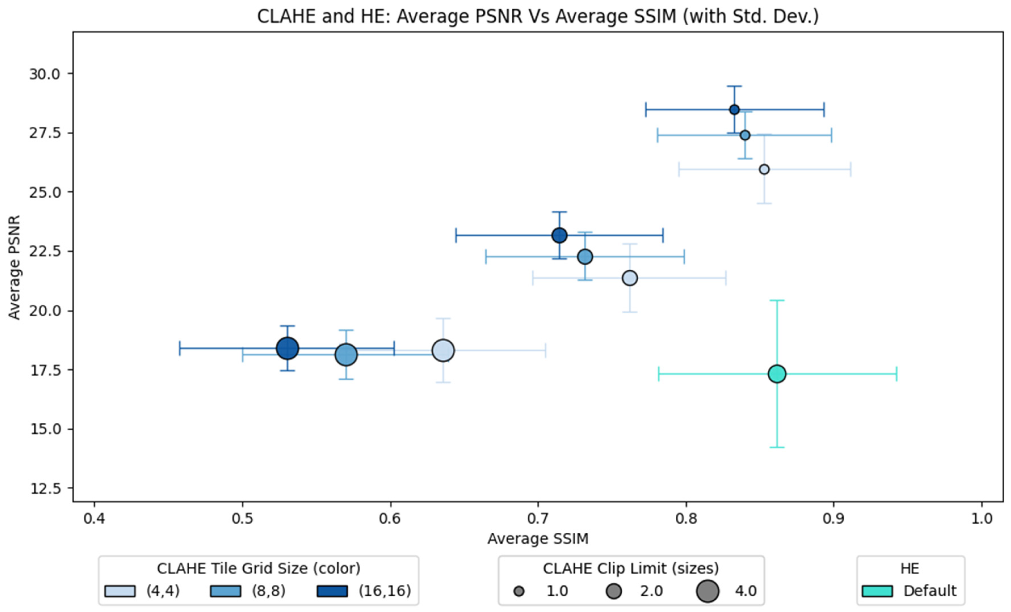
Figure 5 presents a comparative analysis of the CLAHE and HE configurations, evaluating their impact on image fidelity and structural quality. The plot consists of two axes: the average PSNR against the average SSIM for both methods. The lines connected to each point show the standard deviation for each configuration. CLAHE consists of two parameters: tile grid size and clip limit. It is observed that the best clip limit is 1.0, which obtains the highest PSNR and SSIM regardless of the tile grid size. Within the same clip limit (1.0), the tile grid size choice displays a trade-off in terms of average SSIM and PSNR performance. A smaller grid size (4 × 4) displays a higher average SSIM but a lower average PSNR. On the other hand, a larger grid size (16 × 16) has a higher average PSNR but a lower average SSIM. The medium grid size (8 × 8) obtains a balanced performance of the sensitivity metrics. On the other hand, HE achieves polarizing performance on both metrics. Even though HE achieves the highest SSIM compared to all CLAHE configurations, it also obtains the lowest average PSNR. Additionally, HE displays the highest standard deviation for both metrics, indicating high performance variability depending on the image tested.

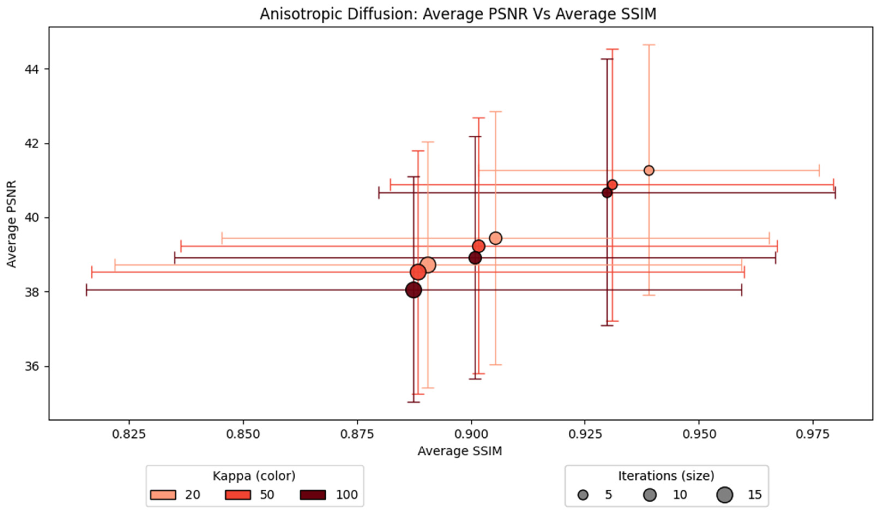
For AD, the number of iterations is observed to influence the average PSNR and SSIM more compared to the kappa value, as displayed in Figure 6. A higher number of iterations applies more smoothing, which reduces the overall image quality. There are three apparent groups for each iteration number. A lower number of iterations performs better compared to higher iterations, regardless of the kappa value. The lowest iteration, which is five, achieves the highest average SSIM and PSNR. Similarly, a lower kappa shows slightly better performance within the same number of iterations. When the number of iterations is five, the plot with a kappa value of 20 achieves the highest PSNR and SSIM. The configuration of a kappa value of 20 and an iteration value of 5 obtains the highest average SSIM and PSNR. Therefore, this configuration is used for our experiment.

4.2. Per-Vertebra Spine Segmentation Results

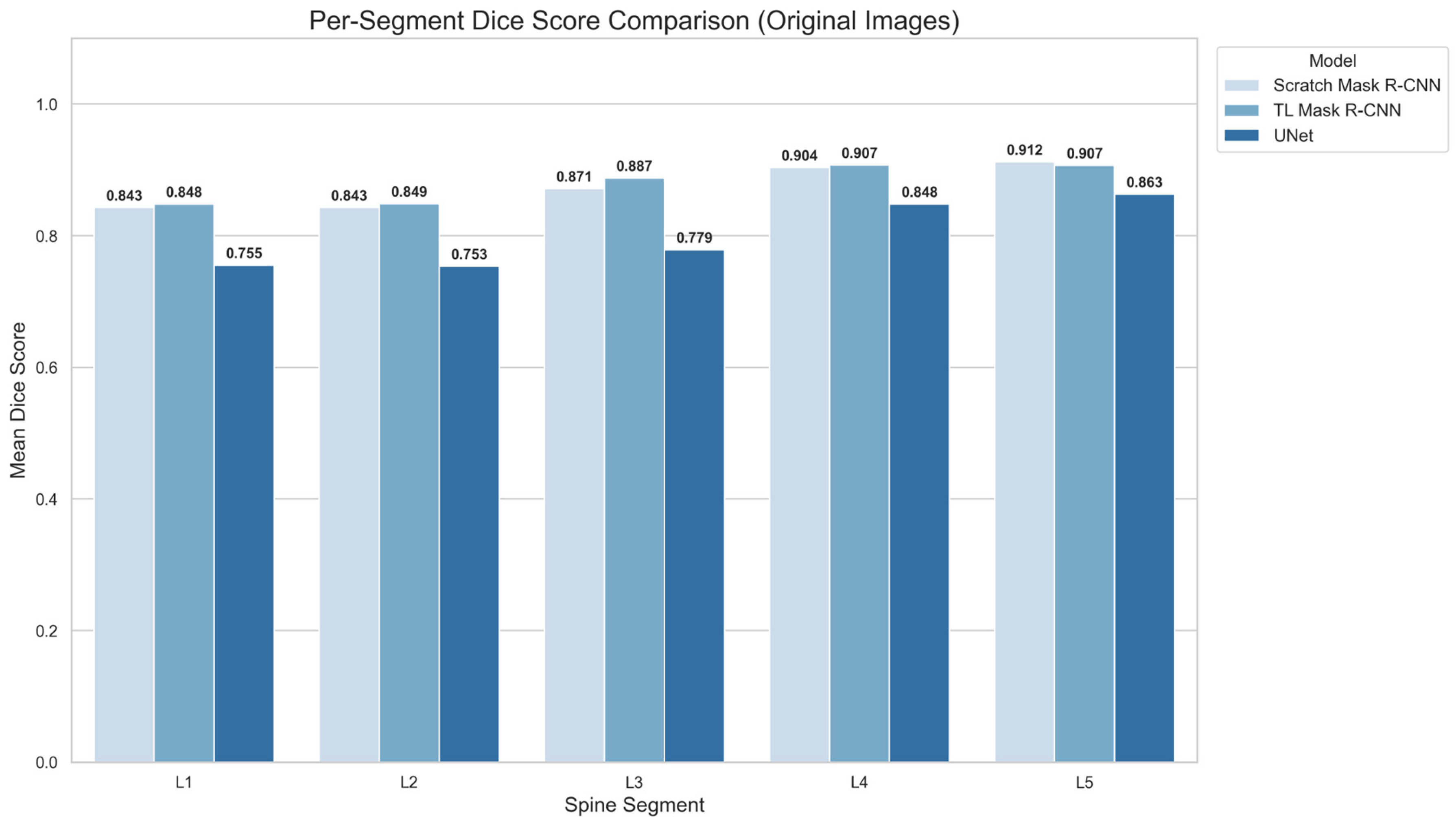
Before the image enhancement is further analyzed, we study the segmentation model’s performance with the original images. Figure 7 displays the bar charts of multiclass segmentation performance on the lumbar spine (L1 to L5) for all the models tested on the original images. L1 and L2 have the lowest mean DSC in all three models. Figure 7 bar charts show that the DSC of L1 and L2 segments is very similar. The TL Mask R-CNN achieves the highest score (DSC: 0.848–0.849), while the randomly initialized Mask R-CNN is slightly lower (DSC: 0.843). However, U-Net trails behind with DSC values of 0.755 and 0.753 on L1 and L2. All models show that the L3 average DSC is higher compared to L1 and L2, but lower compared to L4 and L5. TL Mask R-CNN achieves the highest DSC for L3 (DSC: 0.887), followed by scratch Mask R-CNN (DSC: 0.871) and U-Net (DSC: 0.779).

The scratch Mask R-CNN and U-Net achieved the highest Dice score on L5. In TL Mask R-CNN, the L4 score is identical to L5. The results show that the Mask R-CNN variations maintain comparable performance, ranging from 0.843 for L1 to 0.912 for L5. On the other hand, U-Net DSCs are lower compared to Mask R-CNN for all spine segments, from 0.755 for L1 to 0.863 for L5. Across all configurations, it is apparent that all the models’ mean Dice score increases progressively from L1 to L5.

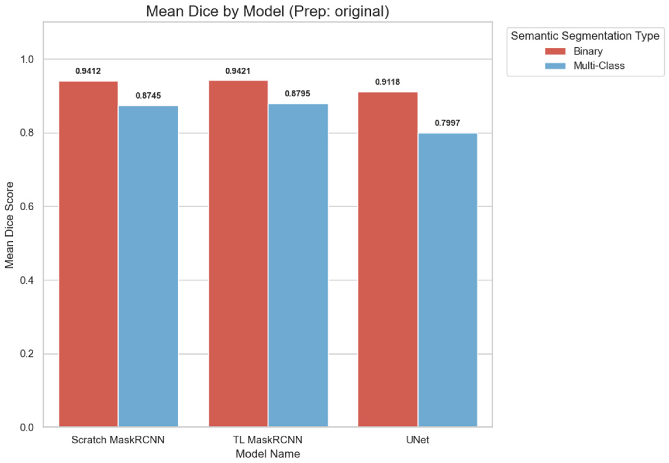
As shown in Figure 8, the binary classification of the spine segments achieved a higher Dice score on all models. Transfer learning Mask R-CNN displays the lowest reduction in performance (0.0626) from binary to multiclass, followed by scratch Mask R-CNN (0.0667). On the other hand, U-Net displays the highest performance reduction of 0.1121. The wide gap between the binary and multiclass semantic segmentation shows that even though the U-Net can detect the spine with a high mean Dice score when combined (DSC > 0.9). However, the model struggles to classify the spine segments correctly, significantly reducing the mean Dice score to less than 0.8.

4.3. Validation-Test Consistency Analysis

Table 2. Comparison of mean Dice score for all fold configurations’ internal validation and external test set.

Model	Internal Validation Mean DSC	External Test Mean DSC	Difference
Scratch Mask R-CNN	0.8871 ± 0.0059	0.8760 ± 0.0041	−0.0110
TL Mask R-CNN	0.8874 ± 0.0054	0.8783 ± 0.0019	−0.0091
U-Net	0.8144 ± 0.0086	0.8062 ± 0.0068	−0.0081

summarizes the internal validation mean DSC compared to the external test mean DSC for multiclass segmentation. The DSC is calculated based on multiclass segmentation. The mean DSC value is calculated as an average from all folds and configurations for all models. The internal and external DSC are closely matched, with absolute gaps below 0.012 across all configurations. The small discrepancies show that the models do not depend on the existence of internal validation sets and are able to generalize consistently with unseen data. Both scratch and transfer learning Mask R-CNN models exhibit nearly identical validation and test performance, suggesting stable feature learning rather than overfitting to the training folds. U-Net shows the same trend, with a mean DSC difference of under 0.01. Overall, the small differences between internal and external results support that overfitting is not a major concern in this study.

4.4. Preprocessing Results Comparison

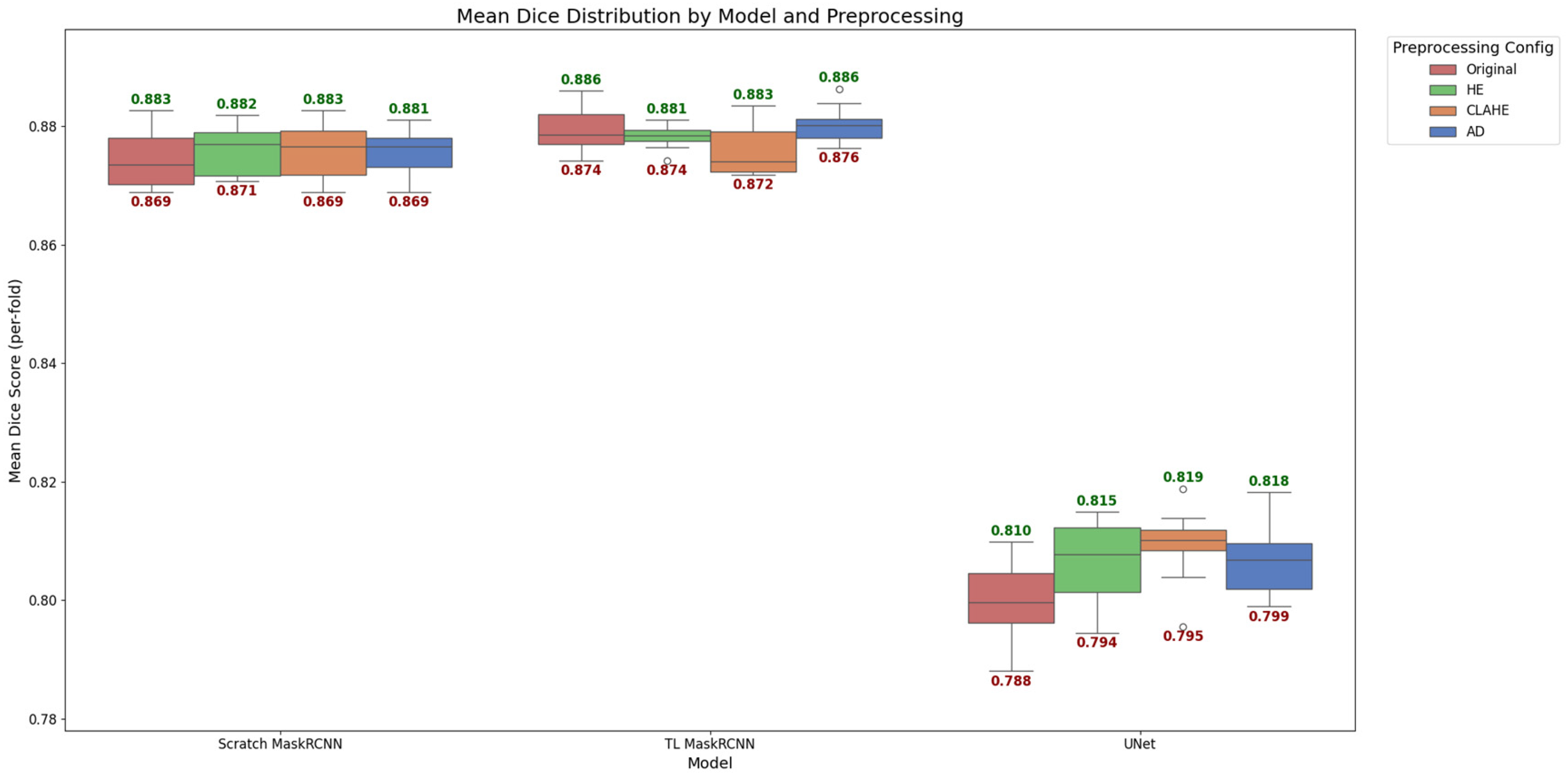
The models are evaluated by comparing the trained models’ prediction segmentation masks using preprocessed image enhancement methods with the ground truth segmentation masks. Each test image is overlaid with the predicted masks to calculate performance metrics. The average values of DSC are calculated, and the box plot results are displayed in Figure 9. The distributions are generated from the ten-fold cross-validation result of the mean multiclass semantic segmentation result.

The box plot in Figure 9 shows that, similar to what is observed in Section 4.2, Mask R-CNN performs better compared to U-Net in both TL and scratch models. The median of the scratch model on all preprocessing configurations is similar to the TL Mask R-CNN, hovering between 0.87 and 0.88. The U-Net model lagged significantly behind, with median scores ranging from 0.80 to 0.82. Notably, TL Mask R-CNN exhibited a tighter interquartile range (IQR) on the HE preprocessing, indicating greater stability and consistency across validation folds. Meanwhile, the scratch model, AD, contributed to a smaller box plot. On the other hand, CLAHE has noticeably improved the performance of the U-Net and contributes to a smaller box. Overall, it is observed that different models’ performance is affected differently by different image enhancement preprocessing methods.

4.5. Statistical Analysis

To evaluate whether preprocessing methods significantly affected spine segmentation performance, the mean Dice score for the multiclass semantic segmentation is used as the primary metric. For each model, Dice scores from ten-fold cross-validation (n = 10) were tested for normality using the Shapiro–Wilk test. All comparisons satisfied the normality assumption (p > 0.05); therefore, a paired t-test was applied to compare each preprocessing method against the corresponding model trained on the original dataset. p-values were adjusted for multiple comparisons using the Holm–Bonferroni correction, and statistical significance is determined at an adjusted p < 0.05.

Table 3. Result Summary.

Model	Method	p-Value	p-Adjusted	Significance
U-Net	AD	0.0195	0.039	True
	CLAHE	0.0095	0.028	True
	HE	0.0856	0.086	False
Scratch Mask R-CNN	AD	0.6378	1.000	False
	CLAHE	0.5947	1.000	False
	HE	0.4252	1.000	False
TL Mask R-CNN	AD	0.6457	0.850	False
	CLAHE	0.1014	0.304	False
	HE	0.4249	0.850	False

summarizes the raw p-values, adjusted p-values, and the significance outcomes of the models trained with specific preprocessing methods. The raw p-values obtained through the paired t-test show that two of the configurations, AD and CLAHE, passed the condition of significance (p < 0.05). Both configurations are trained using the U-Net. The same U-Net configurations remained significant after the Holm–Bonferroni correction. Even though the p-adjusted value of HE on U-Net does not pass the significance threshold, the value (p = 0.086) is marginally significant.

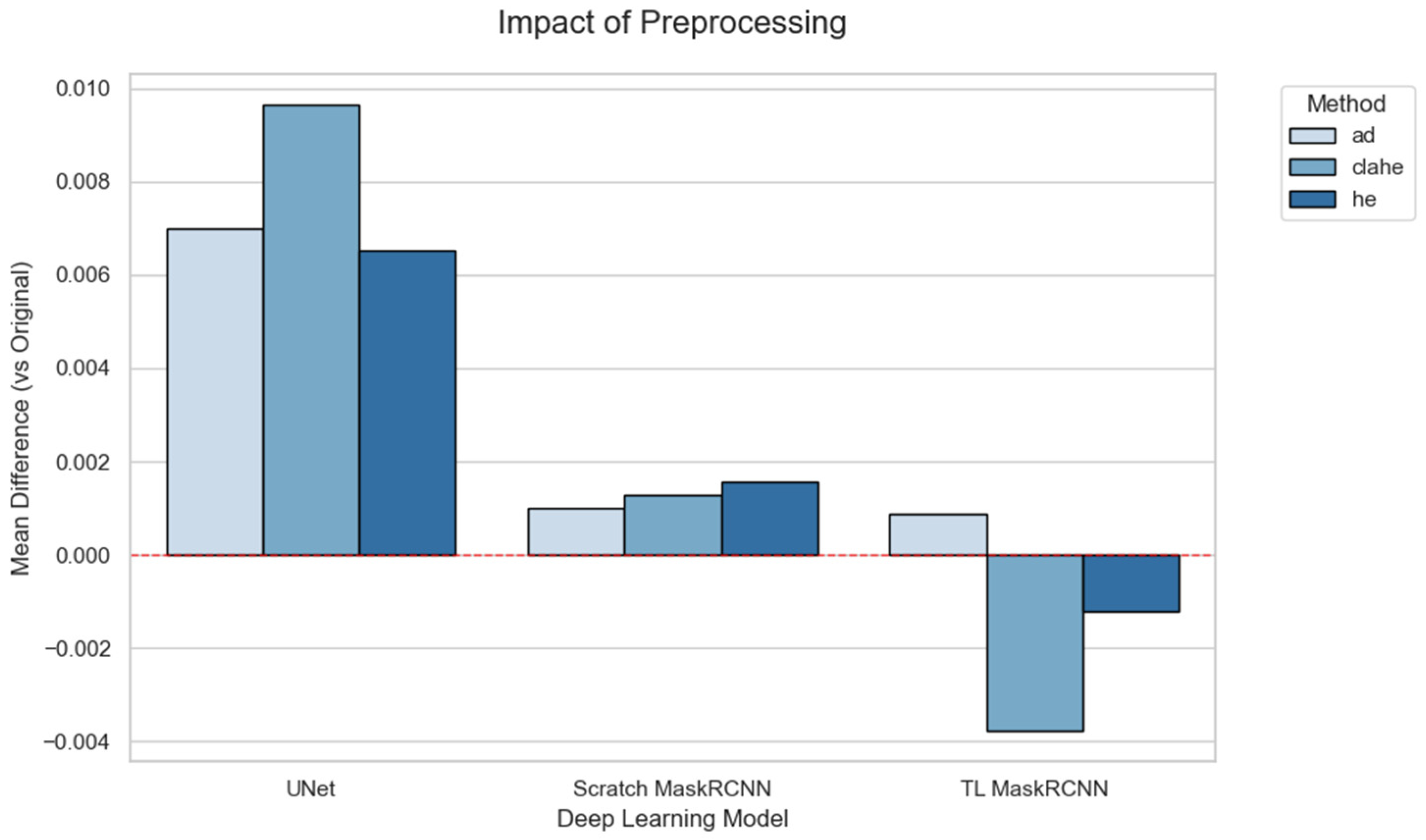
For the scratch Mask R-CNN and TL Mask R-CNN, all the results show that the preprocessing methods do not significantly contribute to the performance of the deep learning models. Scratch Mask R-CNN displays no statistical evidence that preprocessing methods made any difference to the model (p = 1.000). The statistical analysis shows that the preprocessing methods significantly affect the U-Net compared to Mask R-CNN.

Figure 10 visualizes these differences, with bars representing the mean Dice score variation in the preprocessing methods compared to the original image dataset. The plot highlights a considerable improvement in the U-Net compared to Mask R-CNN variations. All the preprocessing methods in the U-Net contribute to positive differences compared to the original images. Scratch Mask R-CNN displays positive differences in all methods. TL Mask R-CNN shows a positive difference in AD. However, CLAHE and HE reduce the mean DSC differences for TL Mask R-CNN.

4.6. Runtime Comparison

Table 4. Total time required for each configuration.

Model	Transfer Learning	Preprocessing Method	Preprocessing Time (ms)	Inference Time (ms)	Total Time (ms)
Mask R-CNN	Yes	None	0.0	180.79	180.79
		AD	17.29	180.79	198.08
		CLAHE	14.87	180.79	195.66
		HE	12.26	180.79	193.05
	No	None	0.0	186.85	186.85
		AD	17.29	186.85	204.14
		CLAHE	14.87	186.85	201.72
		HE	12.26	186.85	199.11
U-Net	No	None	0.0	126.74	126.74
		AD	17.29	126.74	144.03
		CLAHE	14.87	126.74	141.61
		HE	12.26	126.74	139.00

summarizes the inference time, preprocessing time, and total time for all models and preprocessing combinations. Across all configurations, the U-Net achieved a considerably faster inference time compared to Mask R-CNN. U-Net required a mean inference time of 126.74 ms per image, compared to 181–187 ms for Mask R-CNN. This is contributed by the simpler architecture of the U-Net and its fully convolutional design, which requires less computational cost.

Mask R-CNN with transfer learning is slightly faster compared to randomly initialized counterparts. TL Mask R-CNN achieved 180.79 ms, which is 5.86 ms faster compared to scratch Mask R-CNN (186.85 ms). However, this difference is marginal (<6 ms) relative to the inference time.

For both architectures, the addition of any preprocessing methods introduced a small overhead. AD requires 17.29 ms, CLAHE adds 14.87 ms, and HE is the fastest with 12.26 ms. The time for all preprocessing methods is minor (12–17 ms) relative to the inference time (127–187 ms). The fastest configuration is U-Net with no preprocessing at 126.74 ms, followed by other U-Net configurations such as HE, CLAHE, and AD with 139 ms, 141.6 ms, and 144 ms, respectively. This shows that even with the application of preprocessing methods, the U-Net is still considerably faster compared to Mask R-CNN.

4.7. Qualitative Segmentation Visualizations

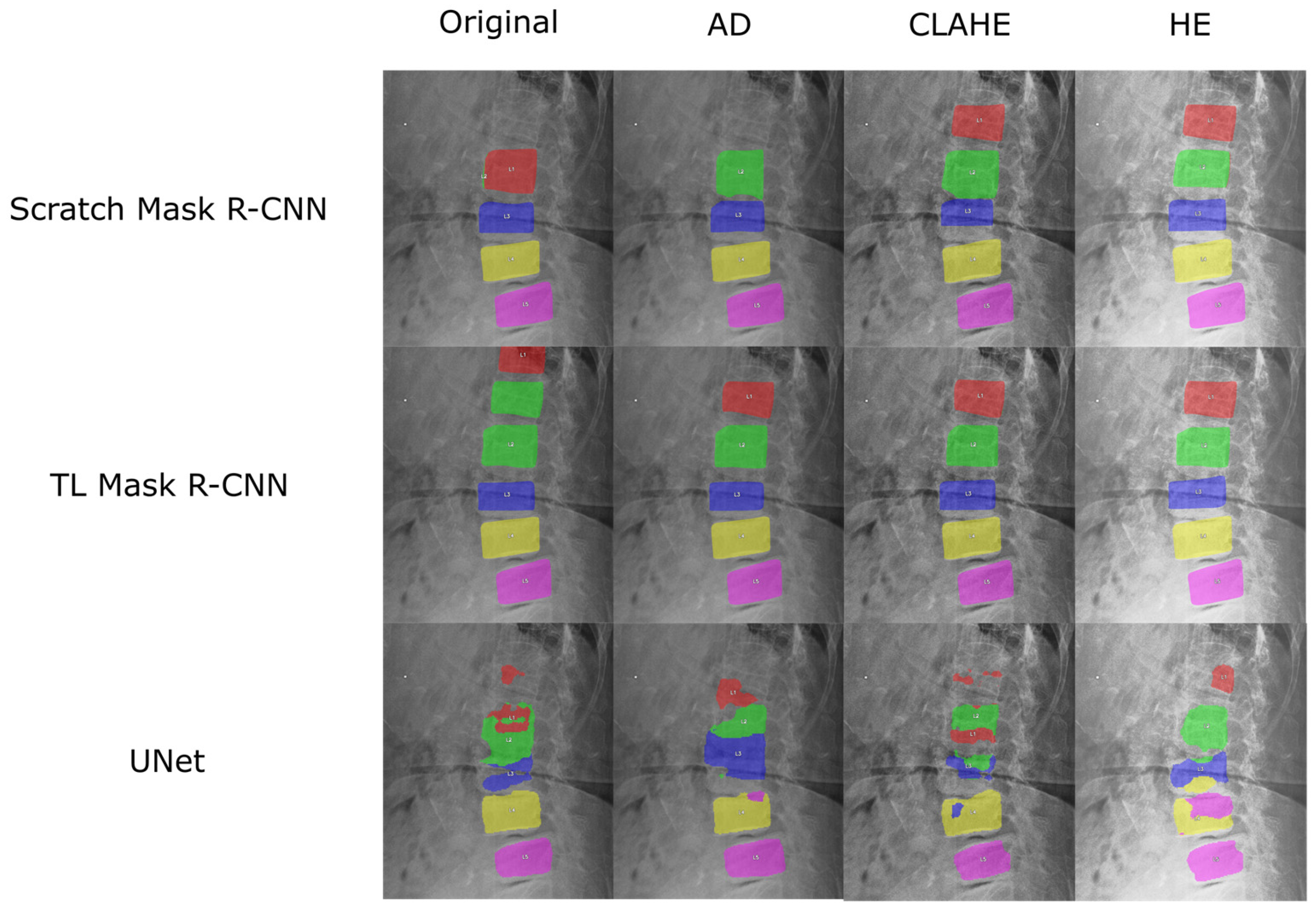
A representative image from the test dataset is selected to evaluate the model’s robustness under challenging conditions, characterized by low contrast and grain noise. As displayed in Figure 11, the segmentation prediction is visualized for each spine segment using different colors. All the Mask R-CNN configurations successfully locate and segment the lower lumbar region (L3, L4, and L5). The application of enhancement methods notably improved performance in the upper lumbar region (L1 and L2). All models using enhanced images correctly predicted L2, and all contrast-enhancement techniques, CLAHE and HE, led to the models successfully segmenting L1. A distinct advantage of TL is observed with AD, where the TL Mask R-CNN correctly identified L1, while the scratch model failed to localize this segment.

Without enhancement, the Mask R-CNN struggles to differentiate the upper vertebrae (L1 and L2). Scratch Mask R-CNN displaying overlapping segmentation errors on the L2 spine segment. Even though the unenhanced TL model correctly labeled the actual L2, it produces a duplicate prediction, mistakenly labeling the L1 as L2. Due to this error, the model misidentified T12 (the lowest thoracic vertebra) as L1.

In contrast, the U-Net segmentation result exhibited significantly inferior performance to Mask R-CNN. Even though U-Net configurations successfully segment the L5, the models failed to consistently segment the remaining vertebrae. For L4, there exists a small area of overlap with neighboring spine segments for AD, CLAHE, and HE. In HE, the model struggles to produce the L4 segment, with L5 prediction overlaps. For upper vertebrae (L1, L2, and L3), the U-Net managed only partial and fragmented predictions.

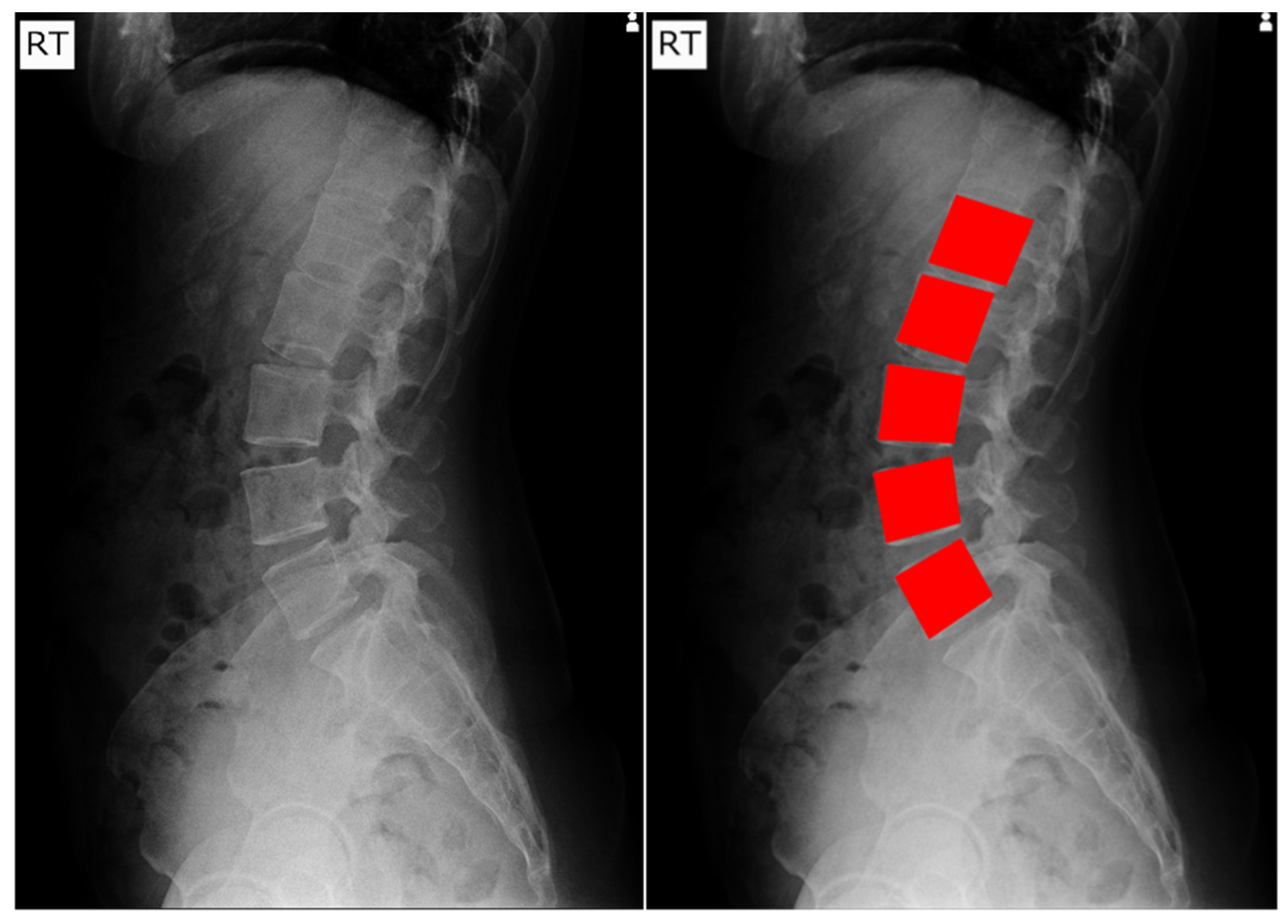
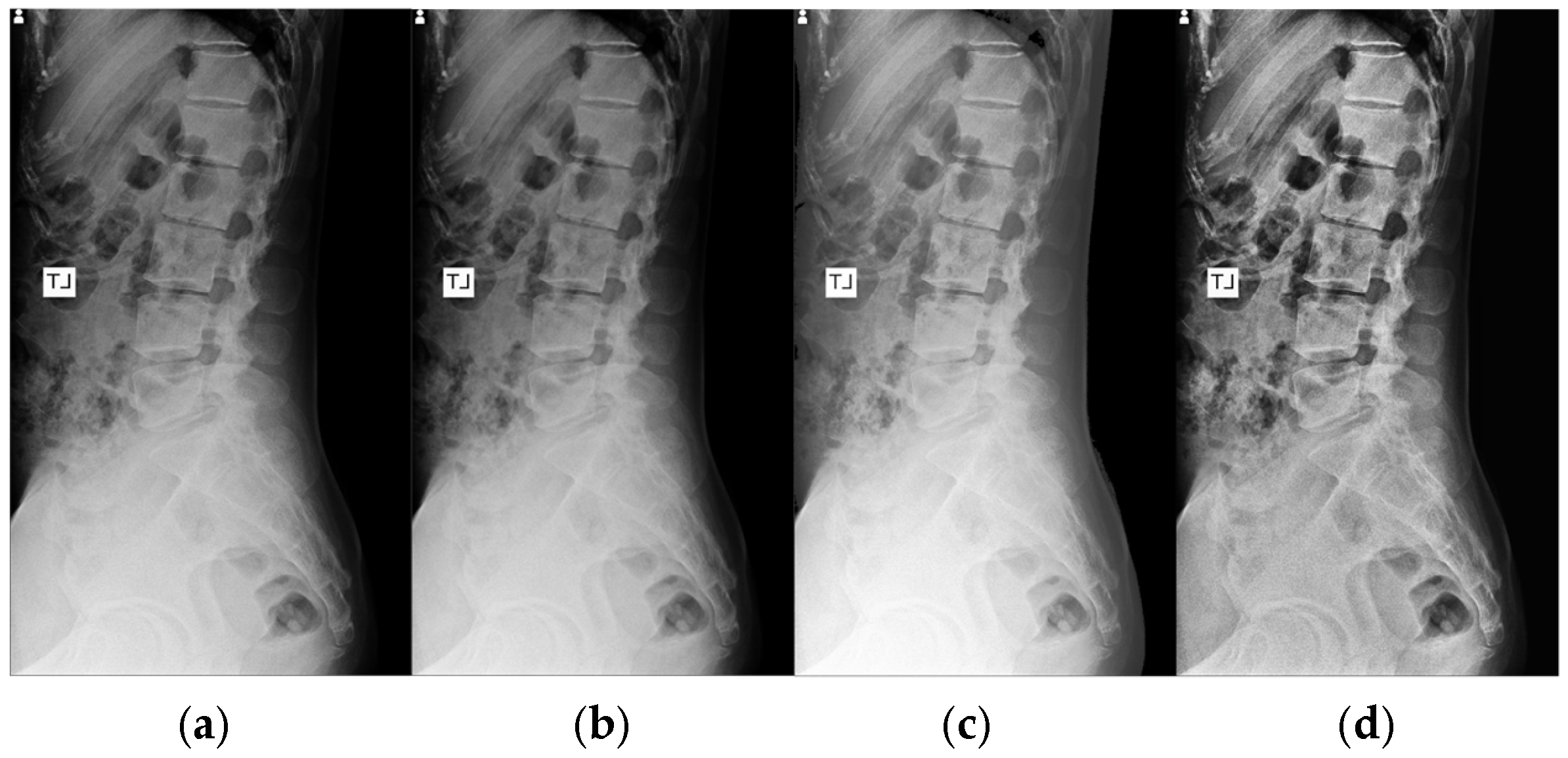
Additionally, three X-ray images were randomly selected, namely 0021-F-079Y1, 4348-F-050Y1, and 4969-F-088Y1. The original and enhanced images are presented to an expert from the orthopedic department. To avoid any bias in judgment, the images are not labeled with their respective enhancement methods, and their order was randomized. The expert was asked to visually assess and rank the clarity of the images for identification of L1 to L5, with 1 being the clearest and 4 being the least clear.

Table 5. Image clarity ranking from expert’s visual evaluation.

	AD	CLAHE	HE	Original
0021-F-079Y1	4	1	2	3
4348-F-050Y1	2	1	3	4
4969-F-088Y1	3	1	4	2
Average	3	1	3	3

lists the rank given to each image. CLAHE-enhanced images are ranked the best for all images. This is similar to what is reported in [15]. The expert noted that the images, after being preprocessed using CLAHE, have the clearest bone outline.

4.8. Comparison with Past Studies

Table 6. Summary of past studies on spine X-ray segmentation using deep learning.

Source	Dataset	Segmentation Type	Model	Transfer Learning	Image Enhancement	Dice Score
[45]	Private (Thoracic and Lumbar)	Binary	CVM-UNet	No	CLAHE and Non-Local Means Denoising	0.911 ± 0.001
[43]	Private (Thoracic and Lumbar)	Binary	Modified U-Net	No	None	0.941 ± 0.034
			Residual U-Net	No	None	0.951 ± 0.027
			Dense U-Net	No	None	0.948 ± 0.028
[46]	Private (Lumbar and Sacrum)	Binary	U-Net	No	Adaptive HE	0.821
[47]	Private (Cervical)	Multiclass	U-Net	No	CLAHE	0.892
[42]	Private (Thoracic and Lumbar)	Binary	Modified U-Net	No	None	0.915 ± 0.006
[44]	Private (Cervical)	Binary	U-Net	No	None	0.910 ± 0.001
			U-Net-S	No	None	0.930 ± 0.001
Ours	Buu Dataset (Lumbar)	Binary	U-Net	No	None	0.912 ± 0.002
					AD	0.915 ± 0.003
					CLAHE	0.916 ± 0.003
					HE	0.916 ± 0.003
			TL Mask R-CNN	Yes	None	0.942 ± 0.001
					AD	0.942 ± 0.001
					CLAHE	0.942 ± 0.001
					HE	0.942 ± 0.001
			Scratch Mask R-CNN	No	None	0.941 ± 0.002
					AD	0.941 ± 0.002
					CLAHE	0.941 ± 0.002
					HE	0.940 ± 0.002

lists the recent literature on deep learning applications for the segmentation of spine radiographs. Most of the articles included in this study only report their model performance on binary segmentation of the spine. Therefore, for fair comparison, our binary segmentation performance is compared. It is worth noting that these studies are using different datasets. The models that appear in all previous work for spine segmentation are based on the U-Net architecture. The listed papers do not include transfer learning in their training pipeline. Additionally, some studies apply image enhancement techniques such as adaptive HE, CLAHE, and Non-Local Means Denoising. However, three papers with the highest Dice score do not include any image enhancement techniques [42,43,44].

Our proposed method using U-Net achieves mean Dice scores ranging from 0.912 to 0.916. On the other hand, scratch Mask R-CNN has a higher mean Dice value, ranging from 0.940 to 0.941. Lastly, our TL Mask R-CNN consistently achieved the highest mean Dice value among our models with 0.942. Horng et al. achieved high Dice scores ranging from 0.941 to 0.951 using three variations in the modified U-Net [43]. Two of the variations, Residual U-Net and Dense U-Net, achieved higher Dice values than ours (0.942 ± 0.001 with TL Mask R-CNN + HE). However, our Mask R-CNN models, across diverse enhancement strategies, have achieved a lower maximum standard deviation of 0.002. The consistency indicates robustness and improved generalization capacity.

5. Discussion

5.1. Comparative Analysis of Segmentation Models

The TL Mask R-CNN achieved the highest performance according to DSC and IoU values compared to all three models. The transfer learning Mask R-CNN was previously trained on the COCO dataset, which increases the model’s ability to generalize to unseen data, which contributes to the overall performance. The Feature Pyramid Network (FPN) of Mask R-CNN, which includes multiscale feature representation using the Feature Pyramid Network (FPN), may contribute to a higher segmentation performance overall and lower improvement due to additional image preprocessing. In a CNN architecture, convolutional layers extract semantic information by reducing the resolution of the feature maps and increasing the number of channels. In the deeper layers, the semantic information and receptive field get higher. However, as the model’s layers get deeper, spatial information is reduced with the resolution of the feature maps. FPN combines the feature maps from the highest to the lowest level, which is explained in more detail in the technical paper of FPN [39]. This process of merging multiple-level features can be represented as a pyramid and enables robust detection at multiple scales.

Additionally, U-Net performs pixel-level segmentation, which is called semantic segmentation, while Mask R-CNN performs instance segmentation [27]. Instance segmentation provides object-level separation that differentiates and creates a segmentation mask for each object. Region proposal networks (RPNs) within the Mask R-CNN architecture propose the candidate object regions after obtaining the feature maps from the FPN. RoIAlign extracts fixed-sized feature maps from Regions of Interest (RoIs). RoIAlign ensures the correct alignment of the extracted feature maps from the ROIs and the original feature maps. This is essential for precise per-instance segmentation prediction in Mask R-CNN. The output of each detected object includes a class label, a bounding box, and a segmentation mask. In summary, the architecture of Mask R-CNN that combines CNN, FPN, RPN, and RoIAlign ensures segmentation results that are more robust to variation in image quality and object size within the input images. The superior performance of instance-aware segmentation results in a higher multiclass segmentation score, as shown in Figure 8. However, due to increased complexity, Mask R-CNN requires more time for inference compared to U-Net, as displayed in Table 4. Even then, the slowest Mask R-CNN configuration only requires 204.14 milliseconds to complete the enhancement and inference process.

The performance gap shown in Figure 8 between binary and multiclass segmentation highlights the increased difficulty of vertebra-level classification. Although all models achieved high Dice scores when treating the lumbar spine as a single structure, separating each segment as an individual class introduces substantial ambiguity due to the highly similar appearance of the lumbar spine. Among the models, Mask R-CNN shows reduced performance degradation due to the multiclass segmentation. This shows that the two-stage instance segmentation architecture framework is more suitable for segmenting and differentiating individual vertebrae. Even though the U-Net produces a competitive result for binary segmentation, the performance degradation is significant when multiclass segmentation is implemented. This shows that a single-stage CNN model struggles to differentiate objects with similar appearances.

A similar result is observed in the work completed by Rettenberger et al. [48]. Mask R-CNN produces more accurate segmentation results on microscopy images compared to the U-Net. In the paper, the authors discovered that Mask R-CNN excels in situations where the target objects, cells, overlap with each other, while U-Net struggles to detect the cells. However, U-Net performs better than Mask R-CNN in situations where the cells are visually not overlapping with each other. This shows that Mask R-CNN may excel in complex situations, but the U-Net is still able to outperform Mask R-CNN in certain scenarios.

5.2. Impact of Image Enhancement Methods

The image enhancement methods affected Mask R-CNN and U-Net algorithms in different ways. According to the statistical analysis, neither of the Mask R-CNN variations displays any significant improvement due to the preprocessing methods. This aligns with Mask R-CNN architecture that consists of a two-stage framework, contributing to the robustness of the Mask R-CNN model to the variations in image quality. This is contributed by an additional ROI detection step using RPN and RoIAlign. This process extracts the rough area for each spine and performs segmentation only on anatomically relevant regions rather than global pixel-level variations. Consequently, Mask R-CNN is less sensitive towards noise or contrast inconsistencies that are commonly observed in X-ray images, leading to minimal performance gains from preprocessing.

In contrast, the U-Net is shown to produce significant improvement on two out of three preprocessing methods evaluated. Both AD and CLAHE produced a significant improvement in Dice score after Holm–Bonferroni correction (p-adjusted < 0.05), indicating that U-Net is highly sensitive to image contrast and noise characteristics. This behavior aligns with its fully convolutional design, where all the pixels in the input images influence the feature extraction. The pixel-level intensity patterns and the presence of noise influence the feature extraction process, reducing the overall performance.

Additionally, higher variations across different image enhancement methods are also present for the U-Net. The model obtained 0.003 on all three methods compared, which is higher than without the image enhancement method (0.002). The reason for this is that the image enhancement method in this experiment is either manipulating the contrast of the images or the noise. However, the images may have varying levels of image quality due to low contrast or noise presence. Contrast improvement methods such as HE and CLAHE may improve contrast levels but amplify the noise. Conversely, AD, a noise-suppressing method, minimizes the noise but reduces fine details in images.

In a broader picture, it is observed that segmentation using enhanced images does not necessarily provide better performance. Image enhancement frequently benefits human observers but may alter the pixels, causing segmentation algorithms to perform worse than with the original data. This is confirmed by the findings [42,43,44] reported in Section 4.3. Another important observation is that the performance of the image enhancement method is model-dependent. A method that is good for a model may result in worse performance for another.

5.3. Impact of Transfer Learning Method

The performance comparison of the TL Mask R-CNN and the randomly initialized Mask R-CNN is discussed in the Section 4. Both the Mask R-CNN variants display a comparable time, with the TL model slightly ahead of scratch Mask R-CNN in all instances. Although the performance difference is small (mean DSC difference < 0.01), the consistent trend supports the hypothesis that the ImageNet initialization provides a beneficial starting point, accelerating learning and leading to a slight but consistent performance gain in X-ray spine segmentation.

In this study, the enhancement methods do not significantly affect Mask R-CNN variants, as shown in Section 4.5. However, upon a closer inspection of the mean DSC difference for CLAHE and HE, the data reveal a polarizing trend depending on the model’s initialization strategy (see Figure 10). While the scratch model shows a marginal performance gain from the methods, the TL model suffers a small performance degradation from the contrast enhancement methods. Although the result is not statistically significant, the difference is likely due to the distinct weight initialization strategy.

The weights of the TL model were optimized for the original ImageNet domain’s color and texture statistics. The application of contrast enhancement methods alters the X-ray images, introducing a domain shift that may reduce the utility of pretrained ImageNet features, whereas the scratch model, having no prior bias, may slightly benefit from the enhanced contrast. This observation aligns with previous work that the efficacy of image enhancement is highly dependent on the model’s architecture and initialization [34].

5.4. Limitations and Future Works

This study covers the performance analysis of established segmentation models and the effects of image enhancement methods on the models in medical images. A limitation of this study is the limited comparison of transfer learning architectures. Due to the lack of open-source, standard implementation using Imagenet-pretrained end-to-end U-Net segmentation models within popular deep learning frameworks, we were restricted to evaluating the non-pretrained U-Net. This constraint ensures reproducibility but prevents a direct comparison to the transfer learning variation in the U-Net.

The experiments provide a baseline understanding of how preprocessing influences the architectures, and the findings can be expanded to the state-of-the-art deep learning models for future research. While U-Net and Mask R-CNN served as the foundational baselines for this study, we acknowledge the emergence of advanced architectures in the recent literature. Recent segmentation algorithms, such as nnU-Net, UNet++, DeepLab V3+, and transformer-based models, consist of complex feature hierarchies and regularization strategies. These models may respond differently to enhancement methods, and future work should evaluate whether the benefits from the methods are significant.

6. Conclusions

This study evaluated three image enhancement techniques for spine segmentation from the BUU-LSPINE X-ray dataset using U-Net and Mask R-CNN architectures. The findings show that different segmentation models are affected differently by image enhancement methods. There is no universal enhancement method that improves all models identified by this study.

A paired t-test is used to assess the significance of image enhancement methods. Two instances of image enhancement methods contribute to the performance improvement of the U-Net algorithms. The methods are CLAHE and AD. However, there is no significant improvement for either Mask R-CNN model. This highlights that the advantage of preprocessing methods is model-dependent.

This study also assesses the effect of transfer learning for Mask R-CNN. The TL Mask R-CNN achieved the highest performance with a Dice score of 0.942 ± 0.001 for binary segmentation and outperformed the non-transfer learning variant across all preprocessing settings. Both the Mask R-CNN models exceed the U-Net performance. Similarly, Mask R-CNN shows superior performance compared to U-Net for multiclass segmentation (DSC: 0.8770–8483), where the U-Net models suffer significant degradation (DSC: 0.8062). The Mask R-CNN’s two-stage architecture contributes to a more robust model. Additionally, the performance variation across enhancement types was smaller compared to past works and all our model variations, suggesting good generalizability. However, U-Net retains a clear advantage in inference speed due to its simpler end-to-end CNN architecture.

Further studies on additional preprocessing methods and more recent architectures, such as nnU-Net, UNet++, DeepLab V3+, and transformer-based models, are necessary to better understand the effects of image enhancement methods in spine X-ray image segmentation using deep learning.